Comprehensive Comparison of Modular Multilevel Converter Internal Energy Balancing Methods - Infoscience
←
→
Page content transcription
If your browser does not render page correctly, please read the page content below
© 2021 IEEE

IEEE Transactions on Power Electronics, pp. 1–1, 2021

Comprehensive Comparison of Modular Multilevel Converter Internal Energy Balanc-
ing Methods

S. Milovanovic and D. Dujic

This material is posted here with permission of the IEEE. Such permission of the IEEE does not in any way imply IEEE
endorsement of any of EPFL’s products or services. Internal or personal use of this material is permitted. However,
permission to reprint / republish this material for advertising or promotional purposes or for creating new collective
works for resale or redistribution must be obtained from the IEEE by writing to pubs-permissions@ieee.
org. By choosing to view this document, you agree to all provisions of the copyright laws protecting it.

POWER ELECTRONICS LABORATORY
ÉCOLE POLYTECHNIQUE FÉDÉRALE DE LAUSANNE
This article has been accepted for publication in a future issue of this journal, but has not been fully edited. Content may change prior to final publication. Citation information: DOI 10.1109/TPEL.2021.3052607, IEEE
                                                                                               Transactions on Power Electronics
          IEEE TRANSACTIONS ON POWER ELECTRONICS

            Comprehensive Comparison of Modular Multilevel
              Converter Internal Energy Balancing Methods
                                      Stefan Milovanović, Student Member, IEEE, Dražen Dujić, Senior Member, IEEE
                                          Power Electronics Laboratory, École Polytechnique Fédérale de Lausanne
                                                     stefan.milovanovic@epfl.ch; drazen.dujic@epfl.ch

                                                                                                                      TABLE I: A short summary of the analyzed balancing methods
             Abstract—Stacking of the floating structures, known as sub-
          modules or cells, provides the modular multilevel converter                                                             Method 1 [11]             Method 2 [12]               Method 3 [13]
          with theoretically unlimited voltage scalability. However, such
          a convenience comes at a price of increased control complexity,                                         Horizontal        SVD-based            Circ. currents ctrl.        Circ. currents ctrl.
          especially in the domain of internal energy control. In other                                           balancing          approach            in the αβ- domain           in the αβ- domain
          words, energies of the submodule clusters must be controlled                                                                                       Injection of
                                                                                                                   Vertical         SVD-based                                        Circ. currents +/−
          to their setpoint values, otherwise, stable and high-performance                                                                              reactive components
                                                                                                                  balancing          approach                                         sequence control
          operation of the converter cannot be ensured. So far, several ap-                                                                               into circ. currents
          proaches towards balancing of the modular multilevel converter
          internal energy, in both vertical and horizontal directions, were
          proposed. Nevertheless, differences among them have never been
          analytically supported. In this paper, three seemingly different                                    excluding the other options mentioned in [4], [5]. According
          energy balancing strategies were thoroughly explained, providing                                    to Fig. 1, a cluster of SMs in series connection with an
          a framework for the theoretical comparison of different dynamic                                     inductor Lbr is referred to as the branch, whereas two branches
          responses provided by them. All the results were verified on the                                    comprise the leg. It is straightforward to notice that the
          large scale hardware-in-the-loop platform, serving as a digital
          twin of a grid connected 3.3kVac/5kVdc, 1.25MW converter being                                      MMC employs distributed and, more importantly, floating DC
          driven by the industrial ABB PEC800 controller.                                                     links. Although the SM represents an independent single-phase
                                                                                                              conversion stage, analysis of the MMC considers every branch
             Index Terms—Modular Multilevel Converter (MMC), Chain-
          link converters, Energy Balancing, Energy Control                                                   to be an entity characterized by its energy storage nature [6],
                                                                                                              [7]. The total energy stored within a branch provides an image
                                                                                                              of voltage across its SM capacitors, consequently, the need for
                                           I. I NTRODUCTION
                                                                                                              the internal energy control becomes evident.
             Owing to the outstanding flexibility and scalability, the                                           The total energy stored inside the MMC can be controlled
          Modular Multilevel Converter (MMC) [1], [2], presented in                                           from either DC or AC terminals, depending on the employed
          Fig. 1, became an attractive solution for vast variety of applica-                                  operating mode (inverter/rectifier). However, equal energy
          tions spanning both Medium Voltage (MV) and High Voltage                                            distribution needs to be ensured in both horizontal and vertical
          (HV) domains. The so-called submodule (SM) represents the                                           directions. Energy exchange among the legs, by means on the
          basic building block of any chainlink converter [3], including                                      suitable circulating current components, which are going to
          the MMC itself. Depending on the application, SMs are                                               be introduced shortly, implies the energy shift in horizontal
          mainly realized as Half-Bridge (HB) or Full-Bridge (FB), not                                        direction. Hence the name horizontal balancing. On the other
                                                                                                              hand, energy exchange between two branches belonging to
                                                                                                              the same leg is referred to as the vertical balancing. Apart
                                                                                                              from ensuring equal energy distribution among the branches,
                                                                                                              the control algorithm must ensure equal distribution of energy
                                                                                                              among the SMs belonging to the same branch. This, however,
                                                                                                              strongly depends on the employed modulator structure, as
                                                                                                              discussed in [8]–[10], and this subject falls out of this paper’s
                                                                                                              scope. Henceforward, the term energy balancing will be used
                                                                                                              to denote the branch/leg energy shifts, while assuming uniform
                                                                                                              energy distribution among the SMs of an observed branch.
                                                                                                                 The subject of energy balancing has been addressed by
                                                                                                              various authors so far, notwithstanding, all the approaches
                                                                                                              known to the scientific community revolve around three main
                                                                                                              ideas summarized in Tab. I, while the term Singular Value
                                                                                                              Decomposition (SVD) will be explained in the upcoming
                                                                                                              sections. For example, energy controllers described in [14]
                                                                                                              or [15], [16] represent an extended variation of the controller
          Fig. 1. Modular Multilevel Converter with the adopted naming convention                             described in [13]. In [17] it was shown that different selection

 0885-8993 (c) 2020 IEEE. Personal use is permitted, but republication/redistribution requires IEEE permission. See http://www.ieee.org/publications_standards/publications/rights/index.html for more information.
                       Authorized licensed use limited to: EPFL LAUSANNE. Downloaded on January 20,2021 at 10:29:16 UTC from IEEE Xplore. Restrictions apply.
This article has been accepted for publication in a future issue of this journal, but has not been fully edited. Content may change prior to final publication. Citation information: DOI 10.1109/TPEL.2021.3052607, IEEE
                                                                                               Transactions on Power Electronics
          IEEE TRANSACTIONS ON POWER ELECTRONICS

          of circulating current optimization criteria leads to the refer-
          ences obtained through the use of controllers from [11], [12].
          Similarly, results already available in [11], [12] were presented
          in [18]. In [19] horizontal balancing principle identical to the
          one described in [11] was proposed, whereas the challenge of
          vertical balancing was solved as discussed in [13].
             Comparison between the approaches described in [11], [12]
          can be found in [20], however, different responses provided
          by the two were never analytically supported nor discussed
          beyond the level of observations. Moreover, despite achieving
          the identical end-goals, energy balancing proposals made in
          [11]–[13] follow completely different lines of thinking and the
          question on what connects them has never been raised before.
          This paper, for the first time, provides a thorough analytic                                        Fig. 2. MMC leg with two Kirchhoff voltage loops. Through a suitable
          connection among balancing methods from [11]–[13] and it                                            manipulation of equations written for both loops, decoupling of the AC and
          can be considered its first contribution.                                                           DC terminal equations can be established. Henceforth, subscripts ”p” and ”n”
                                                                                                              will denote the upper and the lower branch quantities, respectively. Without
             The main goal of [11] was to propose the general concept of                                      the loss of generality, no coupling between the branch inductors is assumed.
          energy balancing in an arbitrary MMC-based circuit. In other
          words, the SVD-based energy balancing method can be used
          in complex structures, such as the Matrix MMC [21] or even                                          procedure for all legs leads to the MMC AC side equivalent
          the MMC operating with parallel branches [22], [23]. Such,                                          circuit depicted in Fig. 3a. As suggested by (2), the average
          rather mathematical, approach is not widely recognized in the                                       value of currents flowing through the branches comprising
          power electronics community and detailed explanation, along                                         an observed leg (4) can be controlled by means of the sum
          with the physical connotation, of the logic underlying it was                                       of voltages created jointly by them. Once again, establishing
          not provided in [11]. Obviously, certain theoretical gaps still                                     the expression (2) for all legs, results in the MMC DC side
          exist and this paper aims at filling them in a comprehensive                                        equivalent circuit presented in Fig. 3b. Without the loss of
          manner, which is considered its second contribution.                                                generality, in both Figs. 3a and 3b, branch resistance was
             The rest of this paper is organized as follows. Sec. II                                          considered negligible.
          provides a brief recapitulation of the MMC operating prin-
          ciples along with the definition of quantities used hereafter.                                                                                           is
                                                                                                                         is = ip − in      (3)         ip = ic +         (5)
          A thorough discussion on the MMC internal energy balancing                                                                                               2
                                                                                                                               ip + in                             is
          approaches can be found in Sec. III, whereas Sec. IV contains                                                  ic =              (4)         in = ic −         (6)
                                                                                                                                  2                                2
          a comprehensive analysis enabling their straightforward com-
          parison. Finally, Sec. V includes results obtained on a large                                          Solving the system of equations (3) and (4) enables a
          scale Hardware-In-The-Loop (HIL) setup serving as a digital                                         different perception of the branch currents and, according
          twin of a 3.3kVac/5kVdc, 1.25MW MMC employing 36 SMs                                                to (5) and (6), branch current can be expressed through
          and operating in the rectifier mode.                                                                a suitable combination of the leg common-mode and AC
                                                                                                              terminal currents. At this point, it is important to state that
                                                                                                              the leg current component defined in (4) has been named
           II. MMC BASIC OPERATING PRINCIPLES AND DEFINITION
                                                                                                              differently within the literature so far. Although known to
                                        OF USED QUANTITIES
                                                                                                              some as the circulating current (e.g. [7], [24]), this component
             Subtraction and addition of equations formed around the                                          will henceforth be referred to as the leg common-mode current
          loops defined in Fig. 2, for an arbitrary MMC leg, provides                                         given that circulating currents will be given another connota-
          (1) and (2), from where one can notice that two independent                                         tion. In a multi-phase MMC, AC terminal currents sum up to
          control quantities can be established.                                                              zero under normal operating conditions. Thus, it is only the leg
                                                                                                            common-mode currents that enter the MMC DC link. For this
              Lbr d             Rbr              vn − vp
                      ip − in +     (ip − in ) =         −vt      (1)
               2 dt              2                  2
                     | {z }                      | {z }
                         i                          vs
                      s
                  d ip + in           ip + in
             2Lbr             +2Rbr            = VDC − (vp + vn ) (2)
                  dt      2              2
                     | {z }                             | {z }
                                 ic                                                     2vc

             The difference between the upper and the lower branch
          current corresponds to the leg AC terminal current (3). Based
          on (1), it can be concluded that this current can be affected
                                                                                                                             (a)                                              (b)
          through the adjustment of the difference between the lower
          and the upper branch voltages labeled with vs . Repeating the                                          Fig. 3.     MMC equivalent circuits seen from: (a) AC side; (b) DC side;

 0885-8993 (c) 2020 IEEE. Personal use is permitted, but republication/redistribution requires IEEE permission. See http://www.ieee.org/publications_standards/publications/rights/index.html for more information.
                       Authorized licensed use limited to: EPFL LAUSANNE. Downloaded on January 20,2021 at 10:29:16 UTC from IEEE Xplore. Restrictions apply.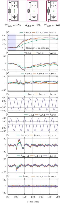
This article has been accepted for publication in a future issue of this journal, but has not been fully edited. Content may change prior to final publication. Citation information: DOI 10.1109/TPEL.2021.3052607, IEEE
                                                                                               Transactions on Power Electronics
          IEEE TRANSACTIONS ON POWER ELECTRONICS

          reason the term ”circulating” was avoided in the process of                                         on several occasions [14], [26]–[28]. Nonetheless, this paper
          naming this current component (common-mode currents leave                                           considers the circulating current components taking part in
          the converter without circulating inside of it, as illustrated in                                   balancing of the mean energy values, rendering the addition
          Fig. 3b). Since the leg-common mode current cannot enter the                                        of higher order harmonics rather irrelevant.
          AC terminal, the decoupled analysis of the leg relevant current                                        By combining (9) with the fact that Fig. 3b presents a
          components can be conducted.                                                                        linear structure, the superposition principle can be applied to
             To introduce the concept of circulating currents, one should                                     the MMC DC equivalent, as presented in Fig. 4. Therefore,
          analyze the circuit from Fig. 3b. By means of the joint                                             voltage component vc0 affects the DC link current/voltage,
          action of three legs, the current entering/leaving the DC                                           while the components vc∆{A/B/C} take part in control of the
          link can be controlled. For the moment, let one assume that                                         legs’ circulating current components. Lastly, as only two out of
          vc{A/B/C} = vc0 . On these terms, ideal distribution of the DC                                      three circulating currents defined above are independent, one
          link current implies that ic{A/B/C} = iDC /3. Unfortunately,                                        can also perceive the circulating currents as the loop currents,
          such a requirement is unlikely to be met for various reasons.                                       which was the approach adopted in [29]. However, it can be
          For instance, identical impedance seen from the DC terminals                                        shown that circulating currents defined as such represent a
          cannot be guaranteed for all the legs. Therefore, expressing                                        linear combination of circulating currents used in [13].
          the leg common-mode current as (7) comes in handy.
                        iDC                                                                                                III. MMC INTERNAL ENERGY BALANCING
                       ic,k =+ ic∆,k , where k = {A, B, C}      (7)
                          3                                                                                     Averaging the MMC leg equations over one AC side
            Summing the legs’ common-mode currents expressed in the                                           fundamental period [6], [7], [24] leads to a straightforward
          above manner, yields                                                                                connection between the leg mean energies and its AC, DC
                                                                                                              and circulating current components. If Wp and Wn denote the
                                      ic∆A + ic∆B + ic∆C = 0.                                        (8)      average value of the total energy stored in the upper and the
                                                                                                              lower branch of an observed leg, respectively, then
             As current components ic∆ do not enter the DC link (they
          sum up to zero), nor are they visible from the AC terminals,                                                              d(Wp + Wn )   dWΣ
                                                                                                                                                =     ≈ VDC Ic∆                                         (11)
          it can be said that they circulate inside of the MMC. For that                                                                dt         dt
          reason, these components will henceforth be referred to as the                                                            d(Wp − Wn )   dW∆
                                                                                                                                                =     ≈ −v̂s î∼
                                                                                                                                                               c∆ .                                     (12)
          circulating currents. In case the expression                                                                                  dt         dt
                                                                                                                 In the above equations, Ic∆ denotes circulating current DC
                                              vc = vc0 + vc∆                                         (9)      part, whereas îc∆ denotes peak of the circulating current AC
             holds for an observed leg, it is can be shown that its                                           component being in phase with the leg AC voltage denoted by
          circulating current can be controlled by means of the voltage                                       vs [24]. According to (11), DC component of the circulating
          component labeled with vc∆ [23]. However, to keep the                                               current affects the total energy (Σ-energy) stored within an
          circulating currents control decoupled from the other MMC                                           observed leg. Hence, it is in charge of the energy balancing
          control layers, the condition                                                                       in horizontal direction. On the other hand, AC component of
                                                                                                              the circulating current affects the energy difference (∆-energy)
                                                                                                              between two branches belonging to the same leg, therefore, it
                                     vc∆A + vc∆B + vc∆C = 0                                        (10)
                                                                                                              governs the vertical balancing process.
             must be satisfied at all times. Without entering into the struc-                                    The first assumption regarding the converter energy balanc-
          ture of the circulating current control methods [25], it must be                                    ing process is that it commences by calculating the circulating
          stressed that (10) holds only if the sum of circulating current                                     current components Ic∆ and îc∆ for each leg individually.
          references equals zero. In general, circulating currents can be                                     However, horizontal and vertical unbalances can take any arbi-
          controlled to zero, however, as will be presented in the next                                       trary values, meaning that simple and independent calculation
          sections, they can be successfully used to achieve the energy                                       of circulating currents in accordance with (11) and (12) might
          balancing among the converter branches. Also, injection of                                          violate the condition defined in (10). Consequently, additional
          higher order harmonics (e.g. 2nd) into the circulating currents                                     reference mapping, which ensures that i∗c∆A +i∗c∆B +i∗c∆C = 0
          with the aim of reducing the SM voltage ripple was proposed                                         must be considered, as indicated in Fig. 5.

          Fig. 4. Decoupling of the MMC DC side equivalent circuit. In case voltage components vc∆ sum up to zero, control of circulating currents (by means of
          voltage components vc∆ ) remains perfectly decoupled from the control of the DC terminal current (by means of voltage component vc0 ).

 0885-8993 (c) 2020 IEEE. Personal use is permitted, but republication/redistribution requires IEEE permission. See http://www.ieee.org/publications_standards/publications/rights/index.html for more information.
                       Authorized licensed use limited to: EPFL LAUSANNE. Downloaded on January 20,2021 at 10:29:16 UTC from IEEE Xplore. Restrictions apply.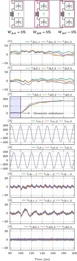
This article has been accepted for publication in a future issue of this journal, but has not been fully edited. Content may change prior to final publication. Citation information: DOI 10.1109/TPEL.2021.3052607, IEEE
                                                                                               Transactions on Power Electronics
          IEEE TRANSACTIONS ON POWER ELECTRONICS

          Fig. 5. The concept of generating circulating current references in the MMC. Mapping of the circulating current references generated in per-leg fashion must
          be performed given that individual control of the leg energies does not guarantee fulfillment of the constraint defined in (10). H∆ (s) and HΣ (s) denote transfer
          functions of controllers being in charge of the energy balance in vertical and horizontal direction, respectively, while vs{A/B/C} = v̂s cos(θ{A/B/C} ). The
          block named Reference mapping converts a set of circulating current references i∗c∆{A/B/C} into a set of new modified references i∗m{A/B/C} ensuring the
          fulfillment of (10) and its effects on the energy balancing dynamics represent the scope of this work.

             Different ways of obtaining a suitable set of circulating                                         always satisfied. Basically, the problem of energy balancing
          currents represent the scope of this paper. Reference [30] con-                                      comes down to the identification of a suitable vector I~M which
          tains an extensive comparison among different MMC internal                                           represents the projection of the original reference I~∗ onto the
          control schemes. However, mapping of the circulating currents                                        null-space of Ti , as illustrated in Fig. 6.
          was not considered. Therefore, a theoretical gap regarding                                             In general, projection of an arbitrary vector ~x onto an
          the effects the circulating currents mapping has upon the                                            arbitrary plane/space (irrespective of its nature) means that
          energy balancing dynamics remained unfilled. In the following                                       ~x should actually be projected onto the basis vectors of the
          paragraphs, mapping approaches used in [11]–[13] will be                                             considered plane/space. A set of vectors B = [b~1 . . . b~k ] is
          discussed in detail and referred to as the Methods 1, 2 and                                          called a basis of a subspace S if
          3, respectively.                                                                                        •   Every vector from S can be synthesized through a linear
                                                                                                                      combination of vectors from B,
          A. Method 1 [11]                                                                                        •   All the vectors from B are linearly independent.
             Even though the control of circulating current DC and                                               Consequently, the heart of balancing strategy discussed here
          AC components can be considered separately, the direction                                           represents the identification of the basis vectors of ker(Ti ). For
          of balancing (vertical or horizontal) will be neglected as the                                      this purpose, the SVD, the explanation of which can be found
          same methodology is adopted in both cases. Therefore, results
          presented henceforward can be considered general.
             As circulating currents were defined in the DC equivalent
          circuit of the MMC, their summation at the DC terminal can
          be formulated as                                                                                             2

                      h        ih                     iT                                                               0
                       1 1 1 ic∆A ic∆B ic∆C = 0.                    (13)                                                                                          –2 –1 0          1    2
                      | {z } |             {z          }                                                              –2
                                  Ti                          I~                                                      –1                                  1

             One can understand that matrix Ti represents the mapping                                                          0                   0
          R3 7→ R, whereas all the vectors I~ being mapped to zero do                                                                 1 –1
          not actually corrupt the MMC DC link current (which indeed
          makes them circulate inside the converter). It is exactly this
          set of vectors that defines the null-space (or kernel, hence
          the label ker(Ti )) of matrix Ti . To put it differently, every                                              2
          possible combination of circulating currents must reside in the
                                                                                                                       0
          null-space of Ti . Nonetheless, energy unbalances among the                                                                                             –2 –1 0          1    2
          MMC branches/legs can take any arbitrary values resulting                                                   –2
          in the control actions violating the constraint of circulating                                              –1                                  1
          current references summing up to zero (please keep in mind                                                           0                   0
          that generation of circulating current references commences                                                                 1 –1
          by performing the balancing of every leg individually). To
                                                                                                              Fig. 6. The concept of generating circulating current references in the MMC
          overcome this issue, a reference vector I~∗ , such that Ti I~∗ 6= 0,                                in case balancing method labeled with 1 is considered. As illustrated, any
          must be projected onto the null-space of Ti , resulting in                                          reference vector I~∗ 6⊂ ker(Ti ) must be projected onto ker(Ti ) in order to
          a modified reference vector I~M , which ensures that (10) is                                        guarantee the fulfillment of (10).

 0885-8993 (c) 2020 IEEE. Personal use is permitted, but republication/redistribution requires IEEE permission. See http://www.ieee.org/publications_standards/publications/rights/index.html for more information.
                       Authorized licensed use limited to: EPFL LAUSANNE. Downloaded on January 20,2021 at 10:29:16 UTC from IEEE Xplore. Restrictions apply.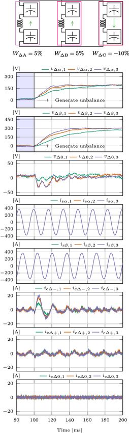
This article has been accepted for publication in a future issue of this journal, but has not been fully edited. Content may change prior to final publication. Citation information: DOI 10.1109/TPEL.2021.3052607, IEEE
Transactions on Power Electronics
IEEE TRANSACTIONS ON POWER ELECTRONICS
in [31], can be used. According to [31], any matrix can be
decomposed as
Ti = U × Σ × V ∗ , (14)
m×n m×m m×n n×n
where V ∗ represents the conjugate transpose of V . If V is
real, V ∗ = V T is true, and (14) can be simplified as Fig. 7. Implementation of the balancing method labeled with 1.
Ti = U × Σ × V T . (15)
m×n m×m m×n n×n
conventional reference frame (which actually is the vector I~M ),
An important property of the SVD is that U and V are the term VNT I~∗ needs to be multiplied by VN , resulting in
unitary (rotation) matrices, while (15) can be expanded as
n−r
X
h
"
i S 0 VT
#" # I~M = VN VNT I~∗ = ~vN,j h~vN,j , I~∗ i. (19)
R
Ti = UR UN r×r T
. (16) j=1
0 0 V N
m×m
n×n
It is worthy to note that, according to [11], previously
m×n
demonstrated procedure is general and it can be applied to
From (16) it can be seen that matrix Σ contains a square any MMC-based converter. The null-space of matrix Ti from
r × r submatrix with elements different than zero and n − r (13) can be identified by firstly creating its SVD form as
zero vectors. The number of zero vectors in Σ corresponds to
the number of orthogonal vectors comprising an orthonormal 1
√1 √1
basis for ker(Ti ). To support such a statement, let one define h i h√ i r 2 √2 2 2
Ti = 1 3 0 0 1 −√12 −√21 . (20)
VN = [~vN,1 . . . ~vN,n−r ] and look for Ti × ~vN,j , such that 3 3
1 ≤ j ≤ n − r, as 0 2 − 23
" #" # From here, it is straightforward to recognize that
h i S 0 VRT
Ti × ~vN,j = UR ~vN,j . (17)
UN r×r
1 0√
VNT
r
0 0 2 1 3
VN = − 2 √2
. (21)
As all the vectors from V are orthogonal according to the 3
− 12 − 23
definition of the SVD, VRT ~vN,j = 0r×n , from where one can
see that Ti~vN,j = 0. As a result, every vector from VN is in Following (19), mapping of the circulating current refer-
the null-space of Ti . Consequently, VN comprises the basis of ences can be performed as
ker(Ti ) since
1 0 0 1 1 1
• All the vectors from VN are in the null-space of Ti , 1
I~M = 0 1 0 I~∗ − 1 1 1 I~∗ . (22)
• All the vectors from VN are independent (moreover, they 3
are orthonormal), 0 0 1 1 1 1
• The number of vectors in VN corresponds to the dimen- Fig. 7 provides graphical illustration of the balancing
sion of the null-space (rank-nullity theorem [31]). approach described in the previous paragraphs. As can be
Once the orthogonal basis of ker(Ti ) is identified, the noticed, circulating current references modification implies
vector demanded by the converter balancing controllers I~∗ the reduction of every individual leg reference by an average
must be mapped to a suitable vector I~M . If basis vectors value of references generated for all the legs individually. It
VN = [~vN,1 . . . ~vN,n−r ] are at disposal, (18) is to be observed is important to notice that the choice of the basis vectors of
at first instance. ker(Ti ) is not unique. Any other orthogonal pair being a subset
of ker(Ti ) could also be chosen (e.g. [20]), without affecting
T
~vN,1
h~vN,1 , I~∗ i
the result obtained in (22). However, a formal proof of such
a statement is omitted as, to the authors’ opinion, it does not
∗ h~vN,2 , I~∗ i
T
~vN,2
VNT I~∗ = I~ = increase the value of results provided above.
.. ..
(18)
. .
T
~vN,n−r h~vN,n−r , I~∗ i B. Method 2 [12]
| {z } 1) Horizontal balancing: In contrast to Method 1, where
scalar products
the energy balancing was performed in the ABC frame,
The vector on the right hand side of (18) contains scalar reference [12] proposes horizontal balancing in the αβ domain
products of orthonormal basis vectors and a balancing refer- by means of relevant power components defined as
ence vector I~∗ . Given that |~vN,k | = 1, these scalar products
actually represent projections of the vector I~∗ onto the basis " # r "
1 1
# PΣA
PΣα 2 1 −√2 −2
vectors from VN . However, these are the coordinates of the = √ . (23)
3 PΣB
3 0 3
vector I~∗ in a new coordinate system consisting of vectors PΣβ 2 − 2
} PΣC
~vN,k . To obtain the coordinates of the new vector in the
| {z
Kαβ
0885-8993 (c) 2020 IEEE. Personal use is permitted, but republication/redistribution requires IEEE permission. See http://www.ieee.org/publications_standards/publications/rights/index.html for more information.
Authorized licensed use limited to: EPFL LAUSANNE. Downloaded on January 20,2021 at 10:29:16 UTC from IEEE Xplore. Restrictions apply.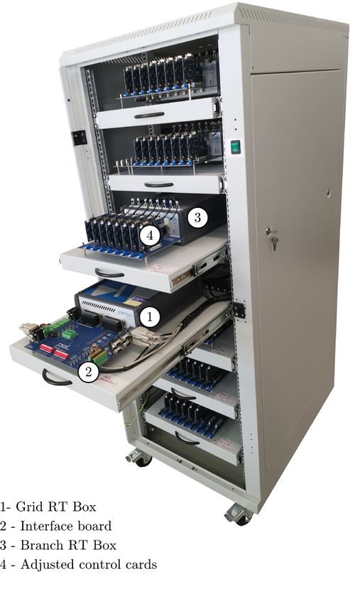
This article has been accepted for publication in a future issue of this journal, but has not been fully edited. Content may change prior to final publication. Citation information: DOI 10.1109/TPEL.2021.3052607, IEEE
Transactions on Power Electronics
IEEE TRANSACTIONS ON POWER ELECTRONICS
Expression (11) establishes the link between power compo- C. Method 3 [13]
nents labeled with PΣ{A/B/C} and their associated circulating 1) Horizontal Balancing: Given that Methods 2 and 3 rely
currents Ic∆{A/B/C} , from where it is easy to see that on the identical principles of horizontal balancing, no further
" # " # discussion is conducted on this matter.
PΣα Ic∆α 2) Vertical Balancing: As can be seen in (21), rows of the
= VDC . (24) matrix used to perform the αβ transformation represent the
PΣβ Ic∆β
bases of ker(Ti ). To a certain extent, this indicates that vertical
Since the vector of circulating currents must remain free balancing, similarly to horizontal, can be performed directly
of any zero-component, otherwise the DC link current gets in the αβ0 domain by means of relevant power components
corrupted, references in the ABC domain can be obtained as being defined as
−√12 −√21
P∆α 1 P∆A
∗
ImA "
∗
# r
2
∗ T Ic∆α
P
= 0 3
− 23 P∆B .
(26)
ImB = Kαβ ∗ . (25) ∆β
3 1
2
∗
Ic∆β P∆0 √ √1 √1 P∆C
ImC 2 2 2
| {z }
Kαβ0
2) Vertical balancing: To commence the desired analysis,
one can take the case presented in Fig. 8 into consideration. As As already discussed, a proper control of converter’s internal
illustrated, the sum of circulating current references generated energies requires identification of circulating current compo-
in ”per-leg” fashion differs from zero. Now, let one observe nents fulfilling this task. Given that ic∆0 = 0, the set of power
phasor ic∆A while neglecting the other two legs’ balancing components P∆ = {P∆α , P∆β , P∆0 } needs to be linked with
references. To perform the cancellation of current defined by the circulating currents expressed in the αβ domain. For that
this phasor in the DC link, two currents can be added into purpose, two dq systems, rotating in the opposite directions,
the legs B and C. What is of crucial importance is that were introduced in [13], giving
current components iA A
c∆B and ic∆C do not contribute to any " # " #" #
active power transfer in the phases they are injected to. For ic∆α cos(θ) − sin(θ) i+ c∆d
instance, iA = +
c∆B denotes the current component injected in the ic∆β sin(θ) cos(θ) i+ c∆q
leg labeled with B with the aim of partially canceling the | {z }
circulating current generated in the leg A. As can be seen, this R+
" #" #
component is orthogonal to the AC voltage vsB . Consequently cos(θ) sin(θ) i− c∆d
only reactive power is generated. This is an important detail , (27)
− sin(θ) cos(θ) i− c∆q
since the reactive power cannot contribute to the change of | {z }
the average energy in any of the converter’s branches. Finally, R−
repeating the same procedure in the other two phases leads where θ = ωs t − γ, which unveils the alignment between
to the final set of circulating current references ensuring the the dq system rotating in the counterclockwise direction and
energy balance in vertical direction. the vector of AC voltages synthesized by the MMC branches.
A set of tedious mathematical steps, which are omitted here
Sum of balancing For an observed phase,
as they can be found in [13], shows that
currents different neutralize its balancing
than zero component by injecting
reactive currents in the 2
adjacent phases P∆α = − √ v̂s i−
6 c∆d
2
P∆β = + √ v̂s i−
c∆q (28)
6
2
P∆0 = − √ v̂s i+ ,
(a) (b)
3 c∆d
from where one can see that the component i+ c∆q can be
Acquire a set of Repeat the procedure
references which sum from (b) in all phases controlled to zero as it does not take part in the control of the
up to zero
above power components. On the other hand, a proper control
−
of circulating current components denoted by i+ c∆d , ic∆d and
−
ic∆q ensures balancing in the vertical direction. Further, as
matrix Kαβ0 from (26) is full-rank, circulating currents in the
ABC domain can be obtained as
(d) (c) i∼∗ " # " #
mA
∼∗ T i+
c∆d T i−
c∆d
Fig. 8. Vertical balancing procedure based on the injection of orthogonal imB = Kαβ R+ + + Kαβ R− − . (29)
components into the circulating currents of all the legs. ic∆q ic∆q
i∼∗
mC
0885-8993 (c) 2020 IEEE. Personal use is permitted, but republication/redistribution requires IEEE permission. See http://www.ieee.org/publications_standards/publications/rights/index.html for more information.
Authorized licensed use limited to: EPFL LAUSANNE. Downloaded on January 20,2021 at 10:29:16 UTC from IEEE Xplore. Restrictions apply.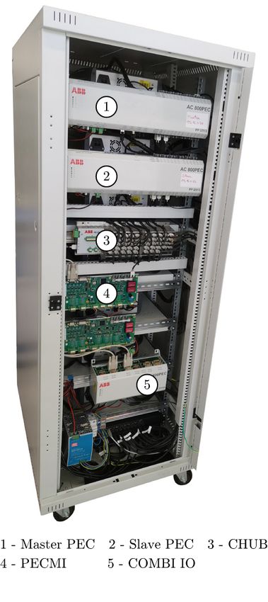
This article has been accepted for publication in a future issue of this journal, but has not been fully edited. Content may change prior to final publication. Citation information: DOI 10.1109/TPEL.2021.3052607, IEEE
Transactions on Power Electronics
IEEE TRANSACTIONS ON POWER ELECTRONICS
IV. M ETHODS C OMPARISON
A. Horizontal balancing ~c∆αβ
∗ = HΣ (s) ~ ∗ ~ ~
V = Wcirc (s) ∗ (W Σαβ − W Σmαβ ) − Ic∆αβ .
VDC
Fig. 9 presents the control block diagram in case control of (34)
all the phases is performed individually (i.e. Method 1). The Expression (34) indicates that horizontal balancing, charac-
expression defining the vector of mapped circulating current terized by the block diagram in Fig. 9, can also be performed
references as in the αβ domain, which was actually proposed in [12], [13].
Furthermore, expression (34) shows that irrespective of the
HΣ (s) ~ ∗ reference frame being used for the generation of circulating
I~M = VN VNT ∗
~ Σm ),
(WΣ − W (30)
VDC current references, the obtained results are the same if identical
=
tuning of controllers HΣ (s) and Wcirc (s) is assumed.
where W ~ Σ = [WΣA WΣB WΣC ]T , along with the leg total
energy controller transfer function being denoted by HΣ (s). To
B. Vertical Balancing
establish the conditions for comparison of previously presented
balancing methods, it is initially assumed that all of them As described in Sec. III, three vertical balancing methods
rely on the identical tuning of controller HΣ (s). Nevertheless, rely on the use of different reference frames. Therefore, prior
identical tuning of the controllers is not mandatory, which will to commencing any further analysis, a common reference
be discussed more in depth in the continuation of this section. frame, from which all the methods can be observed, needs to
Given that the ultimate goal of the MMC control, in general be established. Such a step requires the extension of previously
sense, is to provide references for the upper and lower branch conducted analyses.
voltages, the output of the circulating current controllers is 1) Method 1: By observing Fig. 10, one can notice that,
to be investigated further. In case Wcirc=
(s) denotes circulat- in contrast to the block diagram describing the horizontal
ing current controller transfer function, voltage components balancing, vertical balancing requires the presence of non-
~ ∗ = [V ∗ V ∗ V ∗ ]T can be acquired as ~ where
linear trigonometric terms presented in the form cos(θ),
V c∆ c∆A c∆B c∆C
2π 2π
θA = ωs t − γ (35) θB = θA − (36) θC = θA + (37)
~ ∗ = W = (s) I~M − I~c∆ ,
V c∆ circ (31) 3 3
while ωs and γ denote angular velocity and phase angle
in case filtering and delays in the circulating current of voltage the MMC is synthesizing at its AC terminals,
measurements are neglected. This, however, does not affect respectively. Assuming balanced load conditions, translation
generality of results. Please notice that capital letters denote into the complex domain can be performed, resulting in
that DC components of quantities analyzed in this case, which
is in accordance with (11) and (12).
1 0 0 W∆A
The matrix VNT represents the well p known αβ transforma- H∆ (s) −jγ
~i∼ = VN VNT e 0 a2 0 W∆B ,
(38)
tion with scaling coefficient equal to 2/3 (cf. (26)), hence M
v̂s
(30) can be rewritten as 0 0 a W∆C
| {z }
A
HΣ (s) ~ ∗
I~M = VN ∗ (W ~
Σαβ − WΣmαβ ). (32) 2π
where a = ej . Without the loss of generality, it was
3
VDC ∗ ∗ ∗
assumed that τm ≈ 0, while W∆A = W∆B = W∆C = 0,
Substitution of (32) into (31) yields as vertical unbalances in the legs are normally controlled to
zero. Nevertheless, all the conclusions derived in the upcoming
HΣ (s) ~ ∗
paragraphs remain the same irrespective of the choice of
~ ∗ = ~ ~
Vc∆ = Wcirc (s) VN ∗ (WΣαβ − WΣmαβ ) − Ic∆ , (33) ∗
vertical unbalance references W∆{A/B/C} .
VDC
Mapping of the reference vector ~i∼ c∆ onto the null-space of
while left multiplication of both sides of the above equation matrix Ti implies that Fortescue transformation (39) applied to
with VNT (keep in mind that VNT VN = I), leads to (38), must output only positive and negative circulating current
Fig. 9. Control block diagram of circulating current components maintaining the energy balance in horizontal direction (ABC domain/Method 1)
0885-8993 (c) 2020 IEEE. Personal use is permitted, but republication/redistribution requires IEEE permission. See http://www.ieee.org/publications_standards/publications/rights/index.html for more information.
Authorized licensed use limited to: EPFL LAUSANNE. Downloaded on January 20,2021 at 10:29:16 UTC from IEEE Xplore. Restrictions apply.This article has been accepted for publication in a future issue of this journal, but has not been fully edited. Content may change prior to final publication. Citation information: DOI 10.1109/TPEL.2021.3052607, IEEE
Transactions on Power Electronics
IEEE TRANSACTIONS ON POWER ELECTRONICS
Fig. 10. Control block diagram concerning energy balancing in vertical direction (ABC frame/Method 1)
sequences. To put it differently, zero sequence vector, which
causes the DC link disturbance, must be zero.
1 0 0
W∆A
~i∼ H∆ (s) −jγ
M = e × Mm × 0 a2 0 W∆B (42)
2
1 a a v̂s
1 0 0 a W∆C
Fpn0 = 1 a2 a (39)
3
1 1 1 Left multiplication of both sides of (42) with Fpn0 , gives
Left multiplication of (38) with (39) leads to
√1 W∆0
i∼
m+ 3
∼ H∆ (s) −jγ √2
im− = e × 6 W∆α + jW∆β . (43)
v̂s
√1 W∆0 i∼
i∼
m+ 3 m0 0
∼ H∆ (s) −jγ
im− = e × √16 W∆α + jW∆β ) , (40)
v̂s 3) Method 3: Translating (29) into the complex domain,
i∼
m0 0 followed by the left multiplication with Fpn0 from (39), yields
where Wαβ0 = Kαβ0 WABC . From (40) it can be verified
i+
that zero component of the mapped references indeed corre-
i∼
1 j 0 0 + c∆d
m+
r
sponds to zero. Nevertheless, positive and negative circulating ∼ 2 −jγ ic∆q
im− = e 0 0 1 −j − . (44)
current sequences can be related to the quantities acquired by 3 ic∆d
means of the αβ transformation introduced in (26). Hence, the i∼
m0 0 0 0 0
i−
c∆q
block diagram depicted on the left-hand side of Fig. 11 can
be created. Combining (26) and (28) with the fact that
2) Method 2: A straightforward way to obtain this vertical P∆{α/β/0} = −H∆ W∆{α/β/0} (which is valid according to
balancing method from the block diagram presented in Fig. 10 Figs. 10 and 11, where legs’ delta energy references were set
is to replace the mapping matrix VN VNT with another mapping as zero) along with i+
c∆q = 0, leads to
matrix ∼
im+ √1 W∆0
2
∼ H∆ (s) −jγ
× W∆α + jW∆β .
2
im− = e (45)
1 j √a3 a
−j √ 3 v̂s
∼
a2
j √a3
im0 0
−j 3
Mm = 1 . (41)
√
a a2 Since the components defining the circulating current pos-
j √3 −j √3
1
itive and negative sequence can be expressed in the form
∗
Thereafter, by assuming that τm ≈ 0 and W∆{A/B/C} = 0, presented in Fig. 11, the values of coefficients k+ and k− for
one can establish the expression (42). different balancing methods can be summarized as in Tab. II.
Fig. 11. An alternative way of generating circulating current
√ references
√ achieving the energy balance in vertical direction if balancing Method 1 is considered.
Multiplication constants denoted by k+ and k− equal 1/ 3 and 1/ 6, respectively. The same diagram can be reused in case the other two methods are
analyzed, as will be demonstrated shortly. However, the right-hand side of the figure should be discarded on these terms.
0885-8993 (c) 2020 IEEE. Personal use is permitted, but republication/redistribution requires IEEE permission. See http://www.ieee.org/publications_standards/publications/rights/index.html for more information.
Authorized licensed use limited to: EPFL LAUSANNE. Downloaded on January 20,2021 at 10:29:16 UTC from IEEE Xplore. Restrictions apply.This article has been accepted for publication in a future issue of this journal, but has not been fully edited. Content may change prior to final publication. Citation information: DOI 10.1109/TPEL.2021.3052607, IEEE
Transactions on Power Electronics
IEEE TRANSACTIONS ON POWER ELECTRONICS
TABLE II: Coefficients determining the method used to maintain the energy TABLE III: Values of coefficients determining the balancing dynamics of
balance in vertical direction energy components W∆α , W∆β and W∆0 , respectively.
Method 1 Method 2 Method 3 Coefficient Method 1 Method 2 Method 3
1 1 1
q q
k+ √ √ √
k1α 1 2 2
1
3 3 2 2q3
1 2 q3
k− √ √ 1 1 2 2
6 6 k1β 2q3
1
q3
2 2
k10 3 3
1
As can be observed, vertical balancing methods analyzed so far
differ only in terms of the multiplication constants, whereas
real number, whereas it is controlled to zero in case Method 3
the structure of the control block diagram illustrated on the
is considered, which results in
left-hand side of Fig. 11 remains legit at all times.
Another important remark relates to the tuning of energy r
controllers labeled with H∆ (s). For Methods 1 and 2, energy 3 H∆
i+k+
c∆d =W∆0
balancing commences for every leg individually, meaning that 2 v̂s
r
each leg relies on the use of its own ∆-energy controller. For 3 H∆
every leg, this controller can be tuned differently, however, i−
c∆d = k− W∆α (49)
2 v̂s
such a choice is not reasonable engineering-wise. Hence, r
3 H∆
H∆{A/B/C} (s) = H∆ (s) is adopted. On the other hand, i−
c∆d = − k− W∆β .
2 v̂s
Method 3 relies on the indirect control of legs’ ∆-energies
through the actions being taken in the αβ0 domain. As Systems of equations (28) and (49) can be further con-
α, β and 0 axes are decoupled (orthogonal), three separate nected, giving
controllers can be used for each of the associated energy
components. Even though identical gains can be used for all P∆α = −k− H∆ W∆α = −k1α H∆ W∆α
three controllers, there exists a degree of freedom allowing P∆β = −k− H∆ W∆β = −k1β H∆ W∆β (50)
one to select the gains of controllers Hc∆α (s), Hc∆β (s) and √
Hc∆0 (s) differently. However, such a choice would make the P∆0 = − 2k+ H∆ W∆0 = −k10 H∆ W∆0 .
upcoming comparison rather difficult to follow. Thus, it is It is straightforward to see from the above system
assumed for now that H∆{α/β/0} (s) = H∆ (s). Last but not that the relationship between ∆-energies and relevant
least, the same tuning of controller H∆ (s) is assumed for power components can always be found in the form of
all of the methods analyzed in the next section. It must be P∆{α/β/0} = −k1{α/β/0} H∆ W∆{α/β/0} . Tab. III summa-
emphasized that such a choice is not mandatory. It was rather rizes the values of coefficients k1{α/β/0} depending on the
made to provide the conditions for the comparison of three observed balancing method. According to (28), similar con-
vertical balancing methods analyzed above. Nonetheless, for nection can be established between the αβ0 power compo-
any other tuning of ∆-energy controllers (irrespective of the nents with their associated dq current pairs as P∆{α/β/0} =
analyzed method) the analytic expressions derived above still k2{α/β/0} v̂s ic∆{d− /q− /d+ } . Consequently, the control block
hold, allowing one to conduct a new independent analysis. diagram concerning energy components W∆{α/β/0} can be
provided in a general form, as depicted in Fig. 12. Please recall
C. Comparative analysis that derivation of equations, presented throughout this section,
∗
assumed that W∆ = 0. Notwithstanding, a similar analysis
According to (40), (43) and (45), symmetrical components ∗
could have been conducted in case W∆ took any arbitrary
obtained through the Fortescue transformation of the circulat-
value, which is also indicated in Fig. 12.
ing current references can be in expressed as
It can be assumed that the circulating current controller
ensures aperiodic response in tracking of the negative/positive
H∆ (s) −jγ sequence references, resulting in
i∼
m+ = e × k+ W∆0 (46)
v̂s
H∆ (s) −jγ ∼ 1
i∼ = e × k− (W∆α + jW∆β ), (47) Hcirc (s) =
. (51)
m−
v̂s 1 + sτc
Further, the transfer function of the block denoting filtering
while (44) can be further expanded to obtain the system and measurement of the converter energies depends on the
employed control infrastructure. Nevertheless, the fact that
r r
practical values of this parameter do not exceed 1ms in the
3 jγ ∼ 3 jγ ∼
i+
c∆d =< e im+ +
ic∆q = = e im+ analyzed case allows the Taylor series expansion, yielding
2 2
r r (48)
1 − s τ2m
3 jγ ∼ 3 jγ ∼
i−
c∆d =< e im− −
ic∆q = −= e im− . Hmf (s) = e−sτm ≈ . (52)
2 2 1 + s τ2m
According to (46) and (48), circulating current component The above assumptions do not hinder generality of the
jγ ∼
i+
c∆q equals zero for Methods 1 and 2 since e im+ is always a procedure demonstrated herewith. Conversely, in case Hcirc (s)
0885-8993 (c) 2020 IEEE. Personal use is permitted, but republication/redistribution requires IEEE permission. See http://www.ieee.org/publications_standards/publications/rights/index.html for more information.
Authorized licensed use limited to: EPFL LAUSANNE. Downloaded on January 20,2021 at 10:29:16 UTC from IEEE Xplore. Restrictions apply.This article has been accepted for publication in a future issue of this journal, but has not been fully edited. Content may change prior to final publication. Citation information: DOI 10.1109/TPEL.2021.3052607, IEEE
Transactions on Power Electronics
IEEE TRANSACTIONS ON POWER ELECTRONICS
Fig. 12. A√general control block diagram
√ concerning vertical balancing of the MMC energies. Coefficients k1{α/β/0} can be read from Tab. III, while
k20 = −2/ 3 and k2{α/β} = ∓2/ 6. The advantage of the presented diagram lies in the fact that dynamic analysis of different balancing methods retains
the same analytical form, with the coefficient k1 being the only variable of interest.
and Hmf (s) are found in a different form, a set of steps, similar information on the MMC SMs voltage measurements can be
to the one presented below, can be taken in order to conduct approximated as τm ≈ 375µs.
the comparison of different vertical balancing methods. From here, desired root locus can be constructed as in
If proportional controller is used, then H∆ (s) = kp∆ lead- Fig. 13. Increasing the value of parameter kp∆ causes the poles
ing to a straightforward analysis of the system from Fig. 12 denoted by σ1 and σ2 to approach each other all until a critical
through the Root locus method. Following such a reasoning, point σc , after which these poles slowly start to move towards
one can define transfer function G(s) as the right half-plane, is reached. It is important to notice that,
∼ before this point is reached, σ1 represents the most dominant
Hcirc (s)Hmf (s) N (s)
G(s) = = , (53) pole in the system, thus it determines its dynamic. In other
s D(s) words, the further the pole σ1 from the imaginary axis, the
whereas all the poles of the closed loop transfer function faster the system response (under the assumption of σ1 > σc ).
∗
formed by means of Fig. 12 satisfy the condition To calculate the value kp∆ at which σ1 = σ2 = σc , one can
substitute the solution of
D(s) + kp∆ k1{α/β/0} N (s) = 0. (54)
According to Tab. III, coefficients k1{α/β/0} can take vari- D0 (s)N (s) − N 0 (s)D(s) = 0, (60)
ous values depending on the observed energy component along
with the adopted balancing method. For simplicity reasons, let which is actually s = σc , into
one analyze the energy component W∆0 being controlled by
means of Method 3, while identical procedure can be followed ∗ D(σc )
kp∆ =− . (61)
to analyze other possible combinations. N (σc )
On the above terms, k10 = 1. Thus, if kp∆ → 0, zeros of
the polynomial term D(s), provided in (55) to (57), become Given that (61) represents an expression being quite cum-
poles of the transfer function W∆ /W∆ ∗
. bersome, its analytic form is omitted, however, for recently
adopted parameters τc and τm , it can be calculated that
2 1 ∗
kp∆ ≈ 642. To investigate whether kp∆ ∗
falls within any
σ1 = 0 (55) σ2 = − τ τc
(57) (56) σ3 = −
m realistic range, one can rely on the parameters of an ex-
Similarly, if kp∆ → ∞, poles of the transfer function emplary converter provided in Tab. IV. In this case, nom-
∗
W∆ /W∆ converge towards the zero of the polynomial term inal value of the total branch energy can be calculated as
N (s), which is calculated as ∗ ∗2
Wbr ≈ CSM VbrΣ /(2N ). As an example, one can adopt
∆W∆[p.u] = 10% in order to calculate that, on these terms,
2
n1 = . (58)
τm
At this point, the root locus can be constructed, however, 6
·103
time constants τm and τc can stand in an arbitrary order (e.g.
τm > τc and vice versa). Therefore, to facilitate the root locus 4
construction, parameters of the industrial controller, employed 2
as described in Sec. V, will be relied on. Namely, in case σ3 σ2 σc σ1 n1
Im(s) 0
bandwidth of the circulating current controller is assumed to
∼
match the cut-off frequency of the transfer function Hcirc , then −2
1 −4
τc = . (59)
2πfbw,circ −6
−8 −6 −4 −2 0 2 4 6 8 10 12
In the setup used for verification purposes, fbw,circ ≈ 1kHz Re(s) ·103
was achieved. Without entering into the structure of the
employed controller, the time required for it to obtain the Fig. 13. Root locus constructed based on the function G(s) from (53).
0885-8993 (c) 2020 IEEE. Personal use is permitted, but republication/redistribution requires IEEE permission. See http://www.ieee.org/publications_standards/publications/rights/index.html for more information.
Authorized licensed use limited to: EPFL LAUSANNE. Downloaded on January 20,2021 at 10:29:16 UTC from IEEE Xplore. Restrictions apply.This article has been accepted for publication in a future issue of this journal, but has not been fully edited. Content may change prior to final publication. Citation information: DOI 10.1109/TPEL.2021.3052607, IEEE
Transactions on Power Electronics
IEEE TRANSACTIONS ON POWER ELECTRONICS
√ control of energy components in αβ0 frame. Consequently,
∗
0.1 3Wbr the gains of controllers Hc∆α (s), Hc∆β (s) and Hc∆0 (s)
îc∆0 = kp∆ ≈ 210A, (62)
2v̂s can be selected differently. According to (54), the parameter
determining the position of poles in the transfer function
which is approximately 70% of the converter nominal AC ∗
W∆{α/β/0} /W∆{α/β/0} equals kp∆ k1{α/β/0} . Consequently,
current amplitude. From the MMC hardware design stand- the dynamics guaranteed by Methods 1 and 2 can be obtained
point, such a high value of the circulating current is unaccept- through the use of Method 3 in case tuning of the controllers
able, as it would demand heavy converter oversizing. From according to (63) and (64) is performed.
the control aspect, on the other hand, maximal values of the (method 1/2)
circulating current can be limited by the saturation blocks. (method 3) (method 1/2) k10
∗
Hc∆0 = H∆ × (method 3)
(63)
However, with the proportional gain values as high as kp∆ , k10
the system will always operate in the saturation, making it (method 1/2)
k1{α/β}
(method 3) (method 1/2)
non-linear. Therefore, practical values of the gain kp∆ must Hc∆{α/β} = H∆ × (method 3)
(64)
be set to a significantly lower value compared to the one k1{α/β}
∗
guaranteeing the fastest aperiodic response (kp∆
kp∆ ). From Tab. III, it can be seen that the ratio between
What is more, the same conclusion could be made for all coefficients k1{α/β/0} for Methods 2 and 3 equals
p
the balancing methods considered in this paper, as well as all p 2/3.
This indicates that multiplying the gain kp∆ by 3/2, in
of the energy components W∆{α/β/0} . case Method 2 is considered, leads to the same ∆-energy
So far, identical tuning of the ∆-energy controller has dynamics as if Method 3 is used. Nonetheless, the same cannot
been adopted for all of the analyzed methods. If so, one can be claimed for Method 1. Namely, it can be seen from the first
notice that irrespective of the observed energy component and the third column of Tab. III that the ratio of coefficients
W∆{α/β/0} , the distance between the dominant pole and k1{α/β/0} changes depending on the observedpaxis (α, β or
imaginary axis in the s-plane increases proportionally with 0). For example, multiplying the gain kp∆ by 3/2 leads to
the coefficients k1{α/β/0} (please keep in mind that kp∆ is the response guaranteed by Method 3, however, only in the
fixed). According to Tab. III, these coefficients stand in the case of W∆0 component. ∆-energy response in the α and β
ascending order if moving from methods labeled with 1 to axes would still remain slower compared to Method 3 given
3. This means that, for the identical values of P- controller that the ratio of products kp∆ k1{α/β} for Methods 1 and 3
gain, Method 3 is expected to provide the fastest balancing of remains equal to 1/2 on these terms. Similar analysis can be
∗
energies in vertical direction, at least if kp∆
kp∆ holds. conducted in case identical response in α/β axes is to be
Notwithstanding, identical tuning of energy controllers obtained for Methods 1 and 3. However, the same dynamic
for all the methods is not mandatory, as already discussed response cannot be ensured for W∆0 component.
above. Namely, Method 3 implies independent (decoupled)
1...8
Front Rear
(a) Front view (b) Wiring diagram (c) Rear view
Fig. 14. HIL system employed to validate the results presented throughout the paper.
0885-8993 (c) 2020 IEEE. Personal use is permitted, but republication/redistribution requires IEEE permission. See http://www.ieee.org/publications_standards/publications/rights/index.html for more information.
Authorized licensed use limited to: EPFL LAUSANNE. Downloaded on January 20,2021 at 10:29:16 UTC from IEEE Xplore. Restrictions apply.This article has been accepted for publication in a future issue of this journal, but has not been fully edited. Content may change prior to final publication. Citation information: DOI 10.1109/TPEL.2021.3052607, IEEE
Transactions on Power Electronics
IEEE TRANSACTIONS ON POWER ELECTRONICS
TABLE IV: Parameters of the converter used for results verification purpose
Rated Output Grid Number of SMs Nominal SM SM Branch Branch PWM carrier Fundamental
power voltage voltage per branch voltage capacitance inductance resistance frequency frequency
(S ∗ ) (VDC ) (vg ) (N ) (VSM ) (CSM ) (Lbr ) (Rbr ) (fc ) (fo )
1.25MVA 5kV 3.3kV 6 1kV 3.36mF 2.5mH 60mΩ 1kHz 60Hz
It must be emphasized that the aim of the above discussion controllers were tuned identically as kp{Σ/∆} = 50. Finally,
is not to determine what balancing method provides the best as vertical and horizontal balancing represent two decoupled
performance. On the contrary, the analytic relationships among problems, they are treated separately.
the chosen methods are provided, outlining the ability, but also
the inability in certain cases, to obtain the identical dynamic A. Vertical balancing
responses irrespective of the employed balancing method.
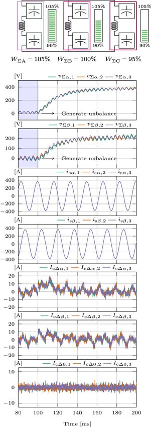
Fig. 15 presents waveforms relevant for comparison of three
Consequently, the freedom to chose the balancing method of
balancing methods in case vertical unbalance scenarios labeled
preference is completely left to the control engineer dealing
with 1, 2 and 3 are observed. As branch voltages are actually
with this subject. Last but not least, throughout the whole
the quantity being measurable, while energies represent a
analysisp conducted above, αβ transformation with coefficient
quantity requiring calculation, the desired comparison includes
Cαβ = 2/3 was used. Nevertheless, for Methods 2 and 3,
Σ- and ∆- leg voltages. Nevertheless, validity of the upcoming
another choice of coefficients (e.g. 2/3 or even 1) can be made.
conclusions is not affected by such a metrics. To facilitate the
In that case, the same analysis can be conducted, however, with
comparison, Σ- and ∆- voltage components were observed
the second
p and third column from p Tab. II being multiplied by through their α, β and 0 components, while subscripts 1,
either 2/3 (Cαβ = 2/3) or 3/2 (Cαβ = 1).
2 and 3 relate a presented waveform with the balancing
method it is associated with. In case the MMC processes
V. HIL VERIFICATION any power, total branch voltages in all the phases feature
As presented in Fig. 14a, the setup used for HIL verification inevitable oscillations. However, for the sake of presenting
purpose comprises 7 RT-Boxes [32] provided by Plexim. 48 how the mean branch/leg energies change, depending on the
SM cards, out of which 36 are used in this case, hosting the employed balancing strategy, these oscillations were filtered
DSP and logical circuitry of the real MMC SM described out from the obtained waveforms.
in [33] were interfaced with 6 RT-Boxes, each containing Fig. 15a provides the waveforms obtained from the em-
the model of an MMC branch. Seventh RT Box (fourth ployed HIL setup in case identical unbalances are generated
from the top in Fig. 14a), contains the model of a grid the in each leg. Consequently, it is evident that the only component
converter is connected to, along with the auxiliary signals being affected is v∆0 . According to Tab. III and (50), when
which are irrelevant for the scope of this paper. In Fig. 14c, voltage/energy component v∆0 /W∆0 is investigated, Methods
two ABB PEC800 controllers can be recognized and they are 1 and 2 are supposed
p to provide identical response as, in both
connected in the Master/Slave structure. The main reason for cases, k10 = 2/3. The third plot from the top validates
such a configuration lies in the fact that several of these HIL such a statement. However, Method 3 provides faster response
systems can be connected to operate in various configurations than two latter methods, which is perfectly aligned with the
(series/parallel MMCs). Therefore, each Slave controller is analyses conducted in Sec. IV-C.
assigned the task of controlling its associated MMC, while An important detail that one should always keep in mind is
one Master controller is to handle general (application) state that energy balancing inside the MMC represents an internal
machine and references. Other parts of the system visible in matter, meaning that it should never be observed from AC
Fig. 14c are in charge of the voltage/current measurements and DC terminals. As can be seen from Figs. 15a to 15c,
(PECMI), distribution of optical signals (CHUB) and manip- intentional generation of ∆-energy (voltage) unbalances does
ulation of relays, switches and other user defined arbitrary not affect the AC terminal currents, expressed through the
signals (COMBIO). It is important to notice that identical Clarke transformation as is{α/β} .
control structure is used in the real MMC prototype making all Further, expression (28) establishes the link between the
of the presented results realistic. Normal operating conditions power components in the αβ0 frame and circulating current
of the MMC imply that the Σ- and ∆-energies are controlled to positive/negative sequences. Accordingly, positive sequence of
WΣ = 1 p.u and W∆ = 0 p.u. Testing of the energy controller circulating current, denoted by ic∆,+ , controls the voltage
responses requires the MMC to be found in a state with the unbalance component being common for all three legs (v∆0 ),
energies deviating from the above setpoints. However, equiv- while negative and zero components get controlled to zero,
alent conclusions can be made in case relevant unbalances as can be confirmed from the last three plots in Fig. 15a. A
are intentionally created. Therefore, three different unbalance very important remark refers to the absence of the circulating
scenarios were defined, as will be seen shortly. The power current current component ic∆0 . Namely, as long as the sum
processed by the analyzed MMC was set to the nominal value, of circulating currents equals zero, no disturbance of the DC
which is, along with the other converter properties, provided link current occurs, which is the main purpose of balancing
in Tab. IV. For all of the inspected balancing methods, energy methods addressed in this work.
0885-8993 (c) 2020 IEEE. Personal use is permitted, but republication/redistribution requires IEEE permission. See http://www.ieee.org/publications_standards/publications/rights/index.html for more information.
Authorized licensed use limited to: EPFL LAUSANNE. Downloaded on January 20,2021 at 10:29:16 UTC from IEEE Xplore. Restrictions apply.You can also read