Order and Information in the Phases of a Torque-driven Collective System

Order and Information in the Phases of a Torque-driven Collective System
 Wendong Wang1†, Gaurav Gardi1†, Vimal Kishore1, Lyndon Koens2, Donghoon Son1, Hunter
 Gilbert1, 3, Palak Harwani1, 4, Eric Lauga5, Metin Sitti1, 6*

1
Physical Intelligence Department, Max Planck Institute for Intelligent Systems, Stuttgart,
Germany.
2
 Department of Mathematics and Statistics, Macquarie University, Australia.
3
 Department of Mechanical and Industrial Engineering, Louisiana State University, United States
of America.
4
 Department of Electronics and Electrical Communication Engineering, Indian Institute of
Technology Kharagpur, India.
5
Department of Applied Mathematics and Theoretical Physics, Cambridge University, United
Kingdoms.
6
 School of Medicine and School of Engineering, Koç University, Istanbul, Turkey.
†
 These authors contributed equally. *Correspondence to sitti@is.mpg.de

Abstract: Collective systems across length scales display order in their spatiotemporal patterns.
These patterns contain information that correlates with their orders and reflects the system
dynamics. Here we show the collective patterns and behaviors of up to 250 micro-rafts spinning
at the air-water interface and demonstrate the link between order and information in the collective
motion. These micro-rafts display a rich variety of collective behaviors that resemble
thermodynamic equilibrium phases such as gases, hexatics, and crystals. Moreover, owing to the
unique coupling of magnetic and fluidic forces, a number of collective properties and functions
emerge as the micro-rafts interact with magnetic potential and nonmagnetic floating objects. Our
findings are relevant for analyzing collective systems in nature and for designing collective robotic
systems.

 1

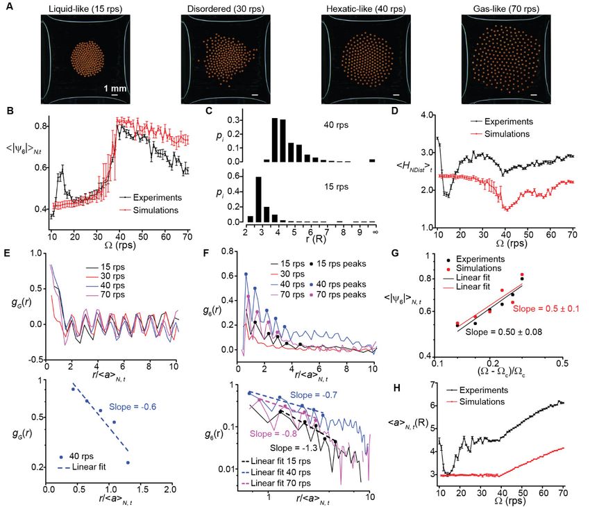
Main Text:
Collective motion in natural or artificial systems displays intriguing patterns with spatiotemporal
orders (1–3). Although inherently out-of-equilibrium, these patterns share similarities with well-
understood states of matter in equilibrium systems and can be considered as phases of the
collectives and characterized by similar metrics (3, 4). In particular, two dimensional (2D) patterns
formed by torque-driven active particles often form structures with hexagonal symmetry (5–8) and
can be characterized by the hexatic order parameter. They resemble the patterns of adenosine
triphosphate (ATP) synthases on cell membranes (9) and of bacteria assembly near interfaces (10).
 The phases of a collective also contain information. This information is embedded in the
structures of the patterns and can be quantified by information entropy (11). Specifically, if we
consider individuals of a collective as the vertices of a graph, the information content of the phase
of a collective could be estimated by graph entropies (12, 13). A similar approach in quantifying
the structural complexity of crystals (14, 15) has given insights into the relationship between
information entropy and thermodynamic entropy (16). The exploration of such information
measures in a collective system will help guide the design of robotic swarms (17–20) and collective
control platforms (21).
 Here we combine the approaches of statistical physics and information theory to analyze the
order and the information in the collective behaviors of hundreds of micro-rafts spinning at the air-
water interface. Our design started with pairwise interactions (Fig. 1 and Movie S1). The three
main pairwise forces are the magnetic dipole-dipole force, the capillary force, and the
hydrodynamic lift force (6) (Fig. 1A). The magnetic dipole is due to the ferromagnetic cobalt thin
film coated on the micro-rafts, and the resulting force and torque depend on the orientation of the
dipole. The angle-averaged magnetic dipole force is attractive. The capillary force and torque
depend on the orientation of the micro-rafts. Their angle-dependence is due to the cosinusoidal
height profiles around the edge of the micro-raft (Fig. 1B – 1E). When the profiles are aligned
(misaligned), the force is attractive (repulsive) (22, 23). The angle-averaged capillary force is
repulsive. The 6-fold symmetry of the structure produces a 6-fold symmetry of the capillary
interaction so that the hexatic order parameter can characterize the structural orders of all phases.
Lastly, the hydrodynamic lift force is always repulsive. We performed experiments in three-
dimensionally (3D) printed enclosures (dubbed “arena” hereafter) inside a custom-made two-axis
Helmholtz coil (fig. S1).
 A pair of micro-rafts orbiting around each other in a steady state undergoes assembling or
decoupling transition as their spin speed decreases or increases, respectively (Figs. 1F – 1G). In
the assembling transition, two micro-rafts align and attach when their spin speed decreases below
a certain threshold (20 rps). It is due to the increase in the
hydrodynamic repulsions at high spin speeds, which results in repulsion at all distances (Figs. 1H
– 1I). Our numerical model, constructed with experimental values and without fitting parameters,
shows close agreement with experiments and validates our hypotheses of the two transitions. (See
Supplementary notes and figs. S2 – S3 for details).
 The pairwise transitions produce two visually striking transitions in the phases of hundreds
of micro-rafts (Movies S2). The decoupling transition causes the transition from disordered to

 2

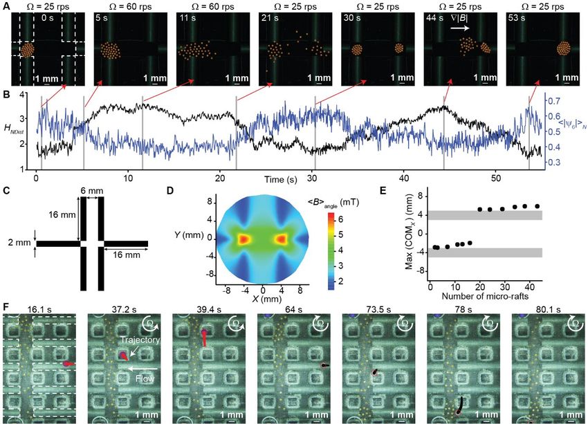
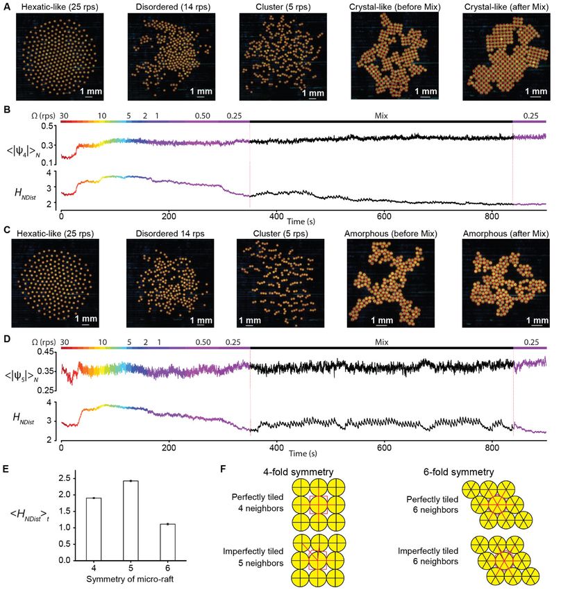
hexatic like-phase, while the assembling transition causes the transition from disordered to the
crystal-like phase.
 The hexatic-like to disordered phase transition (Movie S3) is characterized by the hexatic
order parameter ψ6 (fig. S4A). We first calculate the average of the norms of the hexatic order
parameters N over all micro-rafts (N) in one video frame. For steady states, this number
average was averaged again over time (all video frames), denoted by N,t. Fig. 2A – 2B shows
representative experimental and simulated patterns of the disordered, the hexatic-like, and the gas-
like phases. The disordered to hexatic-like phase transition occurs at ~20 rps and corresponds to a
steep increase in N,t (Fig. 2C). Because the sum of all pairwise forces becomes repulsive at
all distances at 23 rps (Fig. 1I), the interaction between micro-rafts does not oscillate between
attraction and repulsion when the spin speeds reach 23 rps and above, thereby stabilizing the
hexagonal symmetry of the pattern and increasing its hexatic order. The close agreement in the
transition spin speeds between the experiment and the simulation confirms our hypothesis of the
origin of this transition. In equilibrium 2D systems, a hexatic phase possesses short-range
positional order and quasi-long-range orientational order (25, 26). We have found similar
characteristics in the patterns formed at 23 rps (figs. S4), but the relatively small size of the
collective, compared with real thermodynamic systems, precludes a definite conclusion, so we call
this phase hexatic-like.
 The information content of the pattern of a collective is evaluated by the information entropy
of its corresponding graph (12, 13). Each micro-raft is considered as a node or vertex of a graph,
and the connections between neighbors (defined by Voronoi diagram) form edges of the graph.
The information content of a graph depends on the choice of variables. For example, if we select
neighbor count as the variable, then the distribution of its values of all micro-rafts gives a Shannon
entropy. Alternatively, if we select neighbor distance (edge length) as the variable, then the
corresponding distribution has another Shannon entropy. The wide range of variables in a
collective system allows for tremendous flexibility in calculating information entropy. Because
local interactions determine global behaviors in a collective system, characteristics of the global
patterns should manifest themselves in the local environments of individual micro-rafts. Among
the locally-defined variables, we found neighbor distances most useful in differentiating the phases
of micro-rafts collectives.
 Once a variable is selected, we can choose proper binning criteria to construct histograms and
calculate the entropies (Fig. 2D – 2E). We define entropy by neighbor distances =
− ∑ log 2 ( ) , where pi =Xi/X is the probability of a neighbor distance that falls within a
distance interval (a bin) labeled by index i; X is the total count of all neighbor distances of all
micro-rafts, and Xi is the count of the neighbor distances that fall within the distance interval i. For
steady states, HNDist is averaged over time to give t. t captures the transition from
disordered to hexatic-like phase as a decrease at ~20 rps. Intuitively, smaller values of HNDist means
a narrower distribution of the neighbor distances.
 The information entropy reveals features that the hexatic order parameter does not. The sharp
dip of t at 12 rps suggests that the pattern at 12 rps is different from other disordered
patterns. This difference is barely distinguishable in N,t (Fig. 2B). On a concave interface
(fig. S5 and Movie S4), however, a new phase is clearly distinguishable in both N,t and
t. The emergence of this new phase is partly due to the decrease in pairwise distances as
the spin speed decreases and partly due to the gravitational potential created by the concave

 3

interface. In this phase, micro-rafts form a tightly packed structure but are still able to rotate freely
relative to each other without assembling into large clusters, so we call the phase liquid-like.
 While the decoupling transition of the pairwise interaction produces disordered to hexatic-
like transition, the assembling transition accounts for crystal-like phases. Below 10 rps, clusters of
micro-rafts appear and grow, and with a concomitant decrease in the magnetic field strength, the
micro-rafts eventually form a crystal-like phase (Fig. 3A and Movie S5). This phase transition is
due to the pairwise assembling transition. Mixing low magnetic field strengths (1 mT) at low
rotation speeds (

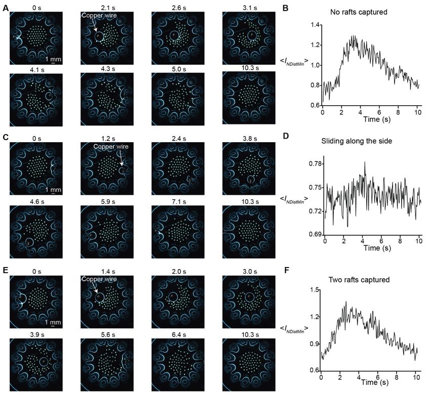
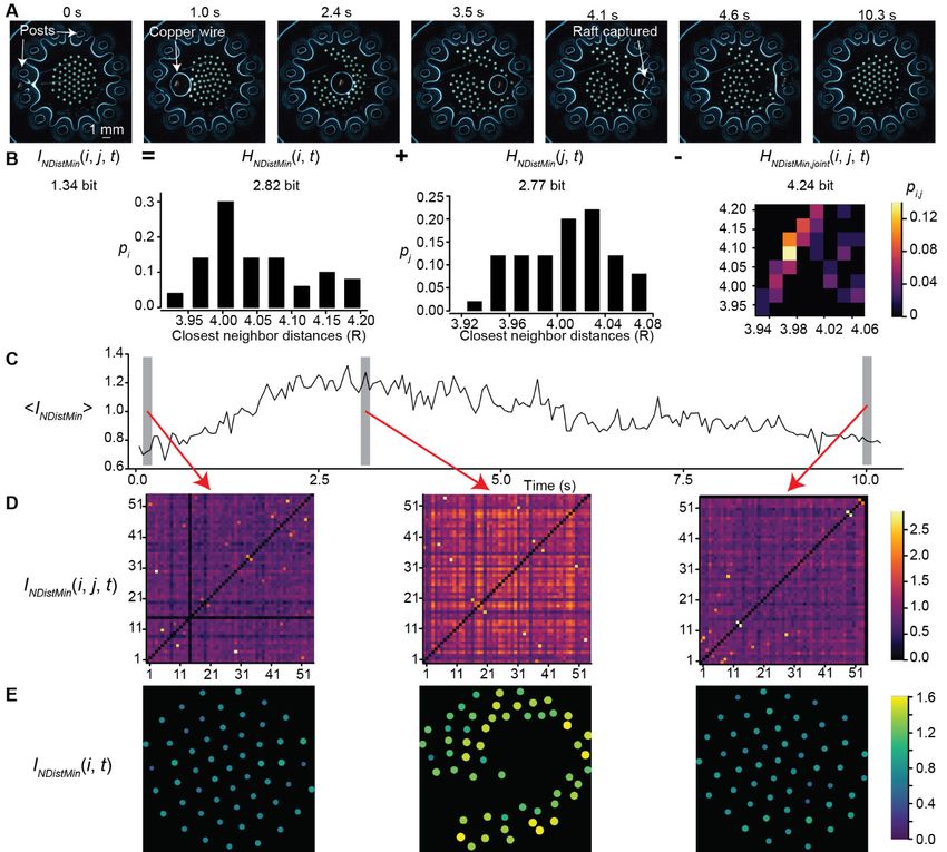
Our preceding analysis suggests that the effect of the angular speed Ω of the rotating magnetic
field on the phases of micro-raft collectives is analogous to the effect of temperature on equilibrium
thermodynamic phases. Although this analogy is not strictly valid (because the magnetic field
strength also influences the phases), it helps rationalize and design collective properties and
functions. As an example, the transition of the hexatic-like phase (a condensed phase) to a gas-like
phase at high spin speeds (high temperature) enabled the micro-rafts (molecules) to cross a
magnetic potential barrier (energy barrier) (Fig. 4A – 4E and Movie S9). Moreover, modifying
the magnetic potential by a gradient (changing the energy landscape) allowed the transport of the
hexatic-like phase as well. Interestingly, we found that only collectives beyond a certain size could
be transported by a magnetic field gradient (Fig. 4E and Movie S10). We surmise that besides the
collective magnetic force and fluctuations in neighbor distances, the surface flows created by the
collective spinning contributed to successful crossings. Again, throughout the entire process, the
order and the information of the collective are inversely related (Fig. 4B).
 A key distinction of the torque-driven collective in its analogy with the thermodynamic
phases is that the rotation speed (temperature) affects the angular (linear) momenta of the micro-
rafts (molecules). The direction of the rotation could be switched to control the interaction between
a collective and its surrounding. For example, both the gas-like phase (Fig. 4E and Movie S11)
and the hexatic-like phase (Movie S12) can redirect the movement of millimeter-sized floating
particles. This function of collective flow guidance works only when the number of micro-rafts is
large.
 Drawing extensive analogies with equilibrium systems, we have shown that the information
entropy of a properly selected variable correlates strongly with the structural order in a collective
system. The experimental system could be used as a model system for testing hypotheses in active
matter, such as non-equilibrium pressure (28). The flexibility in designing magnetic potential with
soft magnetic materials could lead to further emergent collective functions. Moreover, the analysis
of information entropy could be extended to the analysis of mutual information (figs. S9 – S10 and
Movie S13) to investigate temporal structures of collective patterns and to help build collective
robots (29). Coupled with feedback, these information measures could be used to design collective
systems to process information and perhaps to perform computation (30).

 5

References and Notes:
1. P. Ball, Nature’s patterns : a tapestry in three parts (Oxford University Press,
 Oxford ;New York, 2009).
2. F. A. Lavergne, H. Wendehenne, T. Bäuerle, C. Bechinger, Group formation and cohesion
 of active particles with visual perception-dependent motility. Science. 364, 70–74 (2019).
3. T. Vicsek, A. Zafeiris, Collective motion. Phys. Rep. 517, 71–140 (2012).
4. M. E. Cates, J. Tailleur, Motility-Induced Phase Separation. Annu. Rev. Condens. Matter
 Phys. 6, 219–244 (2015).
5. G. M. Whitesides, B. A. Grzybowski, H. A. Stone, Dynamic self-assembly of magnetized,
 millimetre-sized objects rotating at a liquid-air interface. Nature. 405, 1033 (2000).
6. B. A. Grzybowski, H. A. Stone, G. M. Whitesides, Dynamics of self assembly of
 magnetized disks rotating at the liquid–air interface. Proc. Natl. Acad. Sci. 99, 4147–4151
 (2002).
7. Y. Goto, H. Tanaka, Purely hydrodynamic ordering of rotating disks at a finite Reynolds
 number. Nat. Commun. 6, 5994 (2015).
8. W. Wang, J. Giltinan, S. Zakharchenko, M. Sitti, Dynamic and programmable self-
 assembly of micro-rafts at the air-water interface. Sci. Adv. 3, e1602522 (2017).
9. N. Oppenheimer, D. B. Stein, M. J. Shelley, Rotating Membrane Inclusions Crystallize
 Through Hydrodynamic and Steric Interactions. Phys. Rev. Lett. 123, 148101 (2019).
10. A. P. Petroff, X.-L. Wu, A. Libchaber, Fast-Moving Bacteria Self-Organize into Active
 Two-Dimensional Crystals of Rotating Cells. Phys. Rev. Lett. 114, 158102 (2015).
11. T. M. Cover, J. A. Thomas, Elements of Information Theory (John Wiley & Sons, Ltd,
 2006).
12. D. Bonchev, G. A. Buck, in Complexity in Chemistry, Biology, and Ecology, D. Bonchev,
 D. H. Rouvray, Eds. (Springer US, Boston, MA, 2005; https://doi.org/10.1007/0-387-
 25871-X_5), pp. 191–235.
13. M. Dehmer, A. Mowshowitz, A history of graph entropy measures. Inf. Sci. 181, 57–78
 (2011).
14. S. Krivovichev, Topological complexity of crystal structures: quantitative approach. Acta
 Crystallogr. Sect. A. 68, 393–398 (2012).
15. S. V Krivovichev, Which inorganic structures are the most complex? Angew. Chemie Int.
 Ed. 53, 654–661 (2014).
16. S. V Krivovichev, Structural complexity and configurational entropy of crystals. Acta
 Crystallogr. Sect. B. 72, 274–276 (2016).
17. S. Li, R. Batra, D. Brown, H.-D. Chang, N. Ranganathan, C. Hoberman, D. Rus, H.
 Lipson, Particle robotics based on statistical mechanics of loosely coupled components.
 Nature. 567, 361–365 (2019).
18. W. Wang, V. Kishore, L. Koens, E. Lauga, M. Sitti, in 2018 IEEE/RSJ International
 Conference on Intelligent Robots and Systems (IROS) (2018), pp. 1–9.

 6

19. H. Xie, M. Sun, X. Fan, Z. Lin, W. Chen, L. Wang, L. Dong, Q. He, Reconfigurable
 magnetic microrobot swarm: Multimode transformation, locomotion, and manipulation.
 Sci. Robot. 4 (2019).
20. X. Dong, M. Sitti, Controlling two-dimensional collective formation and cooperative
 behavior of magnetic microrobot swarms. Int. J. Rob. Res. (2020),
 doi:10.1177/0278364920903107.
21. G. M. Hoffmann, C. J. Tomlin, Mobile Sensor Network Control Using Mutual
 Information Methods and Particle Filters. IEEE Trans. Automat. Contr. 55, 32–47 (2010).
22. D. Vella, L. Mahadevan, The “Cheerios effect.” Am. J. Phyics. 73, 817 (2005).
23. L. Yao, L. Botto, M. Cavallaro, Jr, B. J. Bleier, V. Garbin, K. J. Stebe, Near field capillary
 repulsion. Soft Matter. 9, 779 (2013).
24. L. Koens, W. Wang, M. Sitti, E. Lauga, The near and far of a pair of magnetic capillary
 disks. Soft Matter. 15, 1497–1507 (2019).
25. D. R. Nelson, Defects and Geometry in Condensed Matter Physics (Cambridge University
 Press, 2002).
26. K. Zahn, R. Lenke, G. Maret, Two-Stage Melting of Paramagnetic Colloidal Crystals in
 Two Dimensions. Phys. Rev. Lett. 82, 2721–2724 (1999).
27. Frederick Reif, Fundamentals of Statistical and Thermal Physics (McGraw-Hill, 1965).
28. G. Junot, G. Briand, R. Ledesma-Alonso, O. Dauchot, Active versus Passive Hard Disks
 against a Membrane: Mechanical Pressure and Instability. Phys. Rev. Lett. 119, 28002
 (2017).
29. H. Hornischer, S. Herminghaus, M. G. Mazza, Structural transition in the collective
 behavior of cognitive agents. Sci. Rep. 9, 12477 (2019).
30. J. M. R. Parrondo, J. M. Horowitz, T. Sagawa, Thermodynamics of information. Nat.
 Phys. 11, 131–139 (2015).

Acknowledgments: We thank Dr. Z. Davidson, Dr. U. Culha, Dr. X. Dong, and Mr. A. Karacakol
for discussions, Dr. A. Pena-Francesch for help with the perturbation experiment, Dr. X. Hu for
magnetic calculations, Dr. G. Ricther and Mr. F. Thiele for help on sputtering and 3D printing of
arenas, Dr. J. Fiene and Mr. B. Wright for 3D printing of the coil frames, N. K.-Subbaiah for help
on Nanoscribe, and Prof. Santhanam and Dr. Malgaretti for feedback on the manuscript. Funding:
We thank the Max Planck Society for funding. W.W. and H.G. thank Alexander von Humboldt
for fellowships and a travel grant; G.G. thanks the International Max Planck Research School for
Intelligent Systems (IMPRS-IS) for support. Author contributions: W.W., G.G., V.K., and M.S.
designed the experiments; W.W., G.G., and P.H. performed the experiments; D.S., H.G., and
W.W. designed the experimental setup; L.K., E.L., and W.W. constructed numerical models;
W.W., V.K., and G.G. wrote the code and performed simulations; W.W., G.G., V.K., and P.H.
analyzed the data; W.W. and G.G. wrote the manuscript; all authors contributed to the editing of
the manuscript; M.S. supervised the research; Competing interests: Authors declare no
competing interests; and Data and materials availability: All data are available in the main text

 7

or the supplementary materials. Video processing and simulation codes will be available in open
source in GitHub.

Supplementary Materials:
Materials and Methods
Supplementary Text
Figures S1-S10
Movies S1-S13

 8

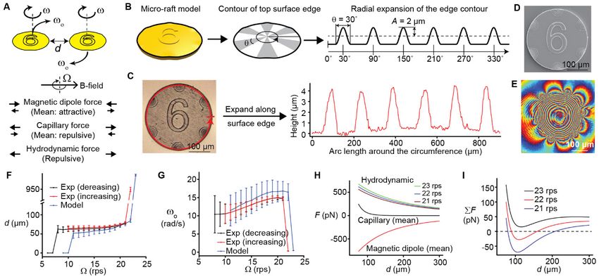
Fig. 1. The design of the pairwise interaction of spinning magnetic micro-rafts. (A) The
scheme of pairwise interactions shows the three main pairwise forces: the magnetic dipole-dipole
force (whose average after one full rotation is attractive), the capillary force (whose average after
one full rotation is repulsive), and the hydrodynamic (lift) force (always repulsive). (B) The
parametric model of one micro-raft. Its surface edge has six cosinusoidal profiles. Each profile has
an arc angle θ of 30° and an amplitude A of 2 µm. (C) The laser confocal image overlapped with
an optical image and the expanded edge height profile showing the six cosinusoidal profiles around
the edge. (D) Scanning electron microscope image of one representative micro-raft. (E) Digital
holographic microscope phase image of one micro-raft on the air-water interface. The deformation
of the interface shows 6-fold symmetry. (F) The edge-edge distance d as a function of the rotation
speed of the magnetic field Ω (in units of revolutions per second (rps)). The experimental curves
are labeled with the direction of change in Ω. The black (red) curve show the assembling
(decoupling) transition. (G) The orbiting speed ωo as a function of Ω. (H) Three main forces as a
function of the edge-edge distance d, calculated from the numerical model. Positive and negative
values correspond to repulsion and attraction, respectively. (I) Sums of the three main forces in
the range of 21 – 23 rps. Error bars in (F – G) correspond to the standard deviation in 2 s of data.

 9

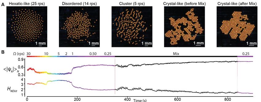
Fig. 2. Phases of a collective of 218 micro-rafts and their order and information. (A)
Representative images of experimental phases. Micro-rafts are marked with red circles to enhance
contrast. (B) Representative images of the simulated phases. (C) The time averages of the number
averages of the norms of the hexatic order parameters N,t as a function of the rotation speed
Ω. (D) Representative experimental probability distributions of neighbor distance at 19 rps and 23
rps. r is the center-to-center distance in units of micro-raft radius R. Each histogram is derived
from all neighbor distances of all micro-rafts in one video frame. (E) Time averages of the
entropies by neighbor distances t as a function of Ω. All error bars correspond to the
standard deviation in 1 s of data.

 10

Fig. 3. Phase transitions of a collective of 251 micro-rafts. (A) Representative images of
different phases. (B) The number averages of the norms of hexatic order parameters N and
the entropies by neighbor distances HNDist as a function of time. The line color indicates the rotation
speed Ω of the applied magnetic field. “Mix” denotes low speeds at a low field strength mixed
with high speeds at a high field strength. See Methods for full procedures.

 11

Fig. 4. Emergent properties and functions. (A) Video frames showing a collective of micro-
rafts interacting with a double-well magnetic potential. The collective first expanded to a gas-like
phase at 60 rps to occupy two wells and then recombined under an oscillating field gradient. Micro-
rafts are marked with red circles. (B) The changes in the order (N) and the information
(HNDist) are inversely correlated during the process. (C) Configuration of the ferrite rods that form
the double-well potential. (D) The simulated angle-averaged in-plane magnetic field strength at 2
mm above the ferrite rods. The potential is proportional to the negative of the field strength, so the
two maxima correspond to the two potential wells. (E) The maximum x-positions of the center-of-
mass of the collectives as a function of the number of micro-rafts. The grey bars indicate the
positions of ferrite rods. (F) Video frames of the gas-like phase redirecting the movement of
floating millimeter-sized plastic beads. The beads are marked by red circles. Their trajectories are
marked by red or black lines. Depending on the direction of rotation of the micro-rafts, the beads
were redirected upwards or downwards. The ferrite rods are marked with white dashed lines in the
first image in (A) and (F).

 12

Supplementary Materials for
 Order and Information in the Phases of a Torque-driven Artificial Collective
 System

 Wendong Wang†, Gaurav Gardi†, Vimal Kishore, Lyndon Koens, Donghoon Son, Hunter
 Gilbert, Palak Harwani, Eric Lauga, Metin Sitti*

 Correspondence to sitti@is.mpg.de

This PDF file includes:

 Materials and Methods
 Supplementary Text
 figs. S1 to S10
 Captions for Movies S1 to S13

Other Supplementary Materials for this manuscript include the following:

 Movies S1 to S13

 1

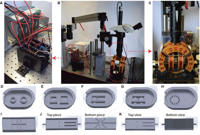
Materials and Methods
Preparation and characterization of the micro-rafts
 Micro-rafts were designed in Rhinoceros 3D with the aid of the Grasshopper plug-in. They
were fabricated on Nanoscribe Photonic Professional GT with a 25x objective and with IP-S
photoresist in the dip-in mode. The slicing distance was set to be adaptive from a minimum of 0.5
µm to a maximum of 3 µm. The hatching distance was 0.3 µm; the hatching angle 45°; hatching
angle offset 72°. The number of contours was 3.
 Thin films of ~500 nm cobalt and ~60 nm gold were sputtered onto the micro-rafts using Kurt
J. Lesker NANO 36. The base vacuum pressure before the sputtering was ~100 µm), whereas the angle-averaged
capillary force dominates in the near field (d < ~30 µm). In the intermediate distances, the balance
between the two main pairwise forces creates a coupled steady state: two micro-rafts orbit around
each other at medium rotation speeds (Ω = ~ 10 – 20 revolution per second (rps))
 Scanning electron microscope (SEM) images of the micro-rafts were taken on EO Scan Vega
XL at 20 kV. Laser scanning confocal microscope images were taken on Keyence VK-X200 series
with a 20x objective. The optical microscope images were taken on Zeiss Discovery V12 using
Basler camera acA1300-200uc. The magnetic hysteresis curves of 500 nm cobalt film sputtered
on a 30-mm-diameter coverslip was measured on MicroSense Vibrating Sample Magnetometer
(VSM) EZ9. Digital holographic microscopy (DHM) images were recorded and analyzed on
Lyncée Tec reflection R2200 with a 5x or 10x objective.
Magnetic rods and 3D printed containers
 The 2-mm diameter ferrite rods (µ = 2300) were purchased from RS electronics. Soft iron rod
of 4 mm in diameter were made of alloy 115CrV3. The containers were 3D printed on Stratasys
Objet 260 Connex. The material used was Vero Clear.

Fabrication and calibration of the electromagnetic coil systems
The custom-built Helmholtz coil system consists of two 5-cm-radius x-coils and two 8-cm-radius
y-coils. The enameled copper wire is 1.41 mm in diameter. The frames of the coil system were
designed in Solidworks and 3D printed by Stratasys Fortus 450mc. The material of the coil frame
is Ultem 1010, which has a high heat deflection temperature of 216 °C. Each coil was driven by
an independent motor driver acting as a current controller (Maxon ESCON 70/10). The power for
the current controllers was supplied by Mean Well, SDR – 960 – 48 (48 VDC at 20 A). The four
motor drivers were connected to the analog output channels of a National Instruments USB-6363,
which was controlled by a LabView program on a PC. The dynamic performance of the current
controllers was tuned manually in the vendor's software Maxon Studio, and the gain and
integration time constants were adjusted so that the commanded currents were able to track signals
up to 100 Hz without noticeable roll-off in magnitude or phase delays.

 2

Each coil was independently calibrated by measuring the B-field in five locations in the
workspace. The mapping was automated using a three-axis stage made of three linear stages
(LTS300 Thorlabs). The measured B-field was used to calculate the current-to-B-field matrix MIB.
Inversion of the MIB gives the B-field-to-current matrix MBI.
 1 
 
 � 2 � = ⎛ ⎞, (1)
 3 / 
 4 ⎝ / ⎠
 −1
 = , (2)
 1
 
 ⎛ ⎞ = � 2 �. (3)
 / 3
 ⎝ / ⎠ 4

 Experimental procedures
 Pairwise experiments (Fig. 1, fig. S3A, S3C – S3D) were performed in the arena of 8 mm
diameter shown in fig. S1D. The air-water interface was kept flat. Videos were recorded in two
sequences, one for each type of transitions: (1) Ω = 10 rps – 22 rps (decoupling transition), in steps
of 1 rps (red curve in Fig. 1F), (2) Ω = 21 rps – 6 rps (assembling transition), in steps of 1 rps,
(black curve in Fig. 1F). The field strength was 10 mT for all sequences. There was a gap of about
60 s between two rotation speeds to allow the micro-rafts to reach steady states. 2 s of data were
recorded for each rotation speed. The magnification of the zoom lens was 2.5x. We also performed
pairwise experiments at other magnetic field strengths (1 mT, 5 mT, and 14 mT). These data will
be reported separately.
 Experiments with 218 micro-rafts (Fig. 2, fig. S4 – S5) were performed in the square arena
with an edge length of 15 mm, shown in fig. S1E. For both flat and concave air-water interfaces,
videos of 1 s were recorded for Ω = 70 rps – 10 rps in steps of 1 rps, and then videos of 20 s were
recorded for Ω = 70 rps – 10 rps in steps of 10 rps. There was a gap of at least 60 s between two
video recordings to allow the micro-rafts to reach steady states. The magnetic field strength was
set to be 16.5 mT to prevent micro-rafts from stepping out. This batch of micro-rafts was produced
in the summer, and its magnetic moment is not as high as those produced in the winter, so a higher-
than-usual field was used. The magnification of the zoom lens was 0.57x.
 The experiments for phase transitions were performed for a collective of 251 spinning micro-
rafts of 6-fold symmetry (Fig. 3 and fig. S6) and for 267 and 198 micro-rafts of 5-fold and 4-fold
symmetries respectively (fig. S7). The air-water interface was kept flat. Videos were recorded for
15 minutes continuously. The magnification of the zoom lens was 0.57x. The rotation speed and
field strength were set according to the list described below for micro-rafts of 6-fold symmetry.
Field strength values in parentheses are for micro-rafts of 4-fold and 5-fold symmetries.
 1. Ω = 30 rps – 20 rps in steps of 5 rps, B = 10 mT (14 mT), 10 s
 2. Ω = 18 rps – 10 rps in steps of 2 rps, B = 10 mT (14 mT), 10 s
 3. Ω = 9 rps – 1 rps in steps of 1 rps, B = 10 mT (14 mT), 10 s

 3

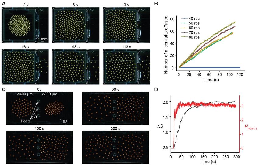
4. Ω = 1 rps, B = 1 mT (10 mT), 30 s
 5. Ω = 0.75 rps, B = 1 mT (10 mT), 30 s
 6. Ω = 0.5 rps, B = 1 mT (5 mT), 60 s
 7. Ω = 0.25 rps, B = 1 mT, 60 s
 8. Mix 1 [Ω = 1 rps and B = 3 mT (10 mT) for 1 s]
 and [Ω = 0.25 rps and B = 0.5 mT (1 mT) for 4 s], 90 s
 9. Mix 2 [Ω = 5 rps and B = 3 mT (10 mT) for 1 s]
 and [Ω = 0.25 rps and B = 0.5 mT (1 mT) for 4 s], 400 s
 10. Ω = 0.25 rps, B = 1 mT, 60 s
 The effusion experiments (figs. S8A – S8B) were performed in the 10-mm square arena with
a 2 mm opening on the right side (fig. S1F). The air-water interface was kept flat. 184 micro-rafts
of 300 µm in diameter were placed in the arena. The rotation speed was initially set to 30 rps, and
the micro-rafts form a hexatic-like phase inside the arena. Videos of 2 min were recorded after Ω
was set to a 40 rps or 50 rps or 60 rps, or 70 rps, or 80 rps. The magnetic field strength was 14 mT.
Effusion occurred only for Ω = 50 rps or higher. The magnification of the zoom lens was 0.8x.
 The mixing experiment (Fig. 4C – 4D) was performed in the arena in fig. S1G with 50 micro-
rafts of 400 µm in diameter and 73 micro-rafts of 300 µm in diameter placed in the left and the
right half, respectively. The air-water interface was kept flat. The rotation speed was initially set
to 30 rps so that the micro-rafts stayed in their respective compartments. One video of 5 min was
recorded after the rotation speed was set to 70 rps. The magnification of the zoom lens was 0.57x.
 The experiments showing the effect of perturbation on the collective (figs. S9 – S10) were
performed in the arena consisting of a ring of posts (fig. S1H). The air-water interface in the arena
was concave. A protruding copper rod was used to perturb the collective of 55 micro-rafts of 300
µm in diameter. Videos were acquired at 500 fps by Phantom MiroLab140 high-speed camera.
Video recordings started when the rod entered the arena and stopped when the collective again
reach steady-state after the rod left the arena. The magnification of the zoom lens was 0.57x.
 Experiments involving the double-well potential (Fig. 4A – 4B) were performed in the arena
shown in fig. S1I. Six ferrite rods of 2-mm diameter were used to create the double-well potential.
43 micro-rafts were transferred to the left well and were rotated at Ω = 25 rps and B = 3 mT. A
single video was recorded for 90 s. Ω and B were changed as the following. First, the magnetic
field rotation speed Ω was changed from 25 rps to 60 rps and kept at 60 rps until some of the
micro-rafts spread over the right well. Then Ω was changed back to 25 rps so that all the micro-
rafts were in either one of the wells. While Ω was kept at 25 rps and B at 3 mT, an oscillating
gradient Bxx·cos(Ωt) with an amplitude Bxx = 2 G/mm was applied to move the micro-rafts from
the left well to the right well. After all the micro-rafts were in the right well, the gradient was
removed to allow the collective to attain steady-state. Finally, an oscillating gradient Bxx·cos(Ωt)
with an amplitude Bxx = - 2 G/mm was used to move all the micro-rafts to the left well, and was
then removed to attain a steady state. The magnification of the zoom lens for the experiment was
0.57x.
 Experiments demonstrating the emergent property in barrier crossing (Fig. 4E) were
performed in the same arena as that for double-well potential. 12 videos of 30 s each were recorded
for 12 collectives having 2, 3, 7, 11, 13, 16, 20, 24, 29, 34, 38 or 43 micro-rafts. The collective

 4

were initially placed on the left well, with Ω = 25 rps and B = 3mT. An oscillating gradient
Bxx·cos(Ωt) with an amplitude Bxx = 2 G/mm was applied to try to move the micro-rafts from the
left well to the right well. After 10 – 15 s, the gradient was set to zero to allow the collective to
attain steady states.
 Experiments demonstrating the emergent function of flow guidance were performed in the
arena shown in fig. S1J. Eight soft iron rods were used to create a potential well at the center of
the arena. A collective of 73 micro-rafts were placed in this well. A video was recorded for 90 s.
The magnetic field B was kept at 10 mT, and a syringe pump was used to create the fluidic flow
from right to left with a low rate of 3 ml/min. The magnetic field rotation speed Ω was set as either
-25 rps or 25 rps in order to direct the flow of polystyrene beads of size 1 mm. For the first control
experiment, the same procedure was repeated without rotating the micro-rafts. For the second
control experiment, only 3 micro-rafts were used.
 Similar methods were used for experiments demonstrating the flow guidance of gas-like
phase (Fig. 4F), with |Ω| = 55 rps and B = 5 mT. 12 ferrite rods were used to create the magnetic
potential. These experiments were performed in the arena shown in fig. S1K.

 Video acquisition and analysis
 Experimental videos were recorded using Basler acA2500-60uc or Phantom Miro Lab140.
The cameras were mounted on Leica manual zoom microscope Z16 APO. LED light source
SugarCUBE Ultra illuminator was connected to a ring light guide (0.83’’ ID, Edmund Optics #54-
176), which was fixed onto the coil frame using a 3D-printed adapter.
 The experimental videos were analyzed with a custom Python code using the OpenCV
library. For pairwise data, the positions and the orientations of the micro-rafts were extracted to
calculate edge-edge distances and angular orbiting speeds. For many-raft data, the positions of
micro-rafts were extracted. Voronoi diagrams were constructed to identify neighbors and to
calculate ψ6, HNDist, and other parameters that characterize structural orders and information
content.
 The hexatic order parameter was calculated according to
 ∑ exp( 6θ )
 6 = , (4)
 
where K is the number of one micro-raft’s neighbors; k is the neighbor index; θk is the polar angle
of the vector from the micro-raft to its neighbor k.
 The spatial correlation of ψ6 was calculated according to
 ∗ ∗
 ⟨ 6, 6, ⟩ ∑ , � − � 6, 6, 
 6 ( ) = = , (5)
 ∑ , � − � ∑ , � − �
where 6, and 6, are the hexatic order parameters of micro-raft j and i, respectively;
∑ , � − � is the normalization factor to ensure that 6 ( ) equals unity at all r for a perfect
crystal of finite size. With this normalization, 6 ( ) is often called bond-orientational correlation
function. In the code implementation, r was set to have increments of 1R, with R being the radius
of micro-raft.

 5

The positional order parameter is denoted by
 , = exp� ∙ � , (6)
where G is one reciprocal lattice vector; rj is the position vector of micro-raft j.
 The spatial correlation of micro-raft positions was calculated according to
 ∗
 ⟨ , , ⟩ ∑ , � − � exp ∙ 
 ( ) = = , (7)
 ∑ , � − � ∑ , � − �
where = − is the vector from the center of micro-raft j to i; ∑ , � − � is the
normalization factor to ensures that ( ) equals to unity at all r for a perfect crystal. In the code
implementation, we reset the origin of the real space to rj to obtain rji for the calculation of
exp ∙ , and looped over all rj as origins. Finally, we averaged all six directions of the
reciprocal lattice and obtain
 1
 ( ) = � ( ) . (8)
 6 
 For the entropy calculation in the many-raft and tiling experiments, the bin edges were r = 2R
– 9.5R in steps of 0.5R and r = ∞, with R = 150 µm. For the mixing experiment, the bin edges
were r = 2R – 9.5R in steps of 0.5R and r = ∞, with R = 175 µm (average of the two radii). For
mutual information calculation in the perturbation experiments, the bin edges were automatically
calculated based on the values in the time series, but the number of bins was kept as 8.
 Simulation (surface evolver, Matlab for capillary calculation, COMSOL)
 The capillary force and torque for edge-edge distances below 50 µm were simulated using
Surface Evolver 2.7. A circle of 1mm in diameter was used as the outer boundary, and the two
micro-rafts were positioned along the x-axis and separated by an edge-edge distance from 1 µm to
50 µm. The orientations of the micro-rafts were kept equal and varied from 0° to 60°. Total surface
energy was obtained as a function of the edge-edge distance and the orientation of the micro-rafts.
The capillary force was obtained as the negative of the derivative of the energy over distance. The
capillary torque was obtained as the negative of the derivative of the energy over the orientation
angle.
 The capillary force and torque for edge-edge distances above 40 µm were computed
according to equations in the section on capillary force and torque calculation in Matlab. The
simulation for pairwise interactions and the collective phases of many rafts were performed
according to equations in the sections on the model for pairwise interactions and model for many-
rafts interactions in Python. In all simulations, the direction of the magnetic dipole is assumed to
coincide with one of the six peaks of the cosinusoidal edge profiles. The angle between the
direction of the magnetic dipole and the x-axis is considered as the orientation of the micro-raft.
 In the pairwise simulations, the initial edge-edge distance of the two micro-rafts was set to be
100 µm, and the initial orientation angles of the two micro-rafts were set to be 0. The time step is
1 ms, and the total time varies between 2 – 50 s. The analysis of steady states was based on the
last 2 s of simulation data. The integration is solved using the Explicit Runge-Kutta method of
order 5(4) in the SciPy integration and ODEs library. We observe that a steady state was usually
reached within 1 s.

 6

In the simulations of collective phases, the initial positions of the rafts were aligned along a
spiral on a square lattice. The center of the spiral is the center of the arena. The spacing between
micro-rafts is 100 µm. The time step is 1 ms, and the total time is 10 s. The integration is solved
using Explicit Runge-Kutta method of order 5(4) in the SciPy integration and ODEs library. We
observe that steady states were reached after 6 – 7 s.
 The simulation of the magnetic flux density profile of ferrite rods (Fig. 4D) was performed
in COMSOL 5.4 with AC/DC model.

Supplementary Text

Supplementary note 1: model for pairwise interactions:
 If the edge-edge distance d ≥ lubrication threshold (=15 µm, or 0.1R)
 2 7
 = �(6 )−1 � − , , � , � + , , � , � + � ̂ 
 3
 ≠ 
 (9)
 − , , � , � 3 
 + �� − 2 � ̂ × z�, = 1,2
 6 
 ≠ 

 sin( − ) − , , � , � + , , � , �
 = + � , = 1,2 (10)
 8 3 8 3
 ≠ 

where and are the position vectors of micro-rafts;
 = − is the vector pointing from the center of micro-raft j to the center of micro-raft i;
 and are the orientations of micro-rafts;
d is the edge-edge distance;
 is the angle of dipole moment with respect to . It is assumed to be the same for both micro-
rafts, as = = in scheme 1 in the section on magnetic dipole force and torque calculation.
 is the instantaneous spin speed of micro-rafts;
 = Ω is the orientation of the magnetic field;
Ω is the rotation speed of the magnetic field;
 is the radius of micro-raft (150 µm);
 is the dynamic viscosity of water (10-3 Pa·s);
 is the density of water (103 kg/m3);
 is the magnetic dipole moment of the micro-rafts (10-8 A·m2);
 is the magnetic field strength (10 mT);
 − , , and − , , are the magnetic dipole force on and off the center-to-center axis,
respectively, and they are functions of and ; (See the section on magnetic dipole force and
torque calculation for details)

 7

 − , , is the magnetic dipole torque, and it is a function of and ; (See the section on
magnetic dipole force and torque calculation for details)
 , , is the capillary force, and it is a function of and and embeds the symmetry of a
micro-raft: (See section on capillary force and torque calculation for details)
 , , is the capillary torque, and it is a function of and and embeds the symmetry of a
micro-raft. (See section on capillary force and torque calculation for details)
 If the edge-edge distance d < lubrication threshold (=15 µm, or 0.1R) and d ≥ 0,
 2 7
 = � � � � − , , � , � + , , � , � + � ̂ 
 3
 ≠ 
 
 + � � � − , , � , � ̂ × z� (11)
 
 ≠ 
 
 + � � � sin( − ) ̂ × z�, = 1,2
 
 ≠ 

 = � � sin( − )
 
 (12)
 + � � � − , , � , � + , , � , � , = 1,2
 
 ≠ 

where the coefficients are defined as the following (S. Kim, S. J. Karrila, Microhydrodynamics
(Butterworth-Heinemann, 1991)):
 (−0.285524 + 0.095493 ln( ) + 0.106103 )
 ( ) = (13)
 
 1 1
 �0.0212764 ln � � + 0.157378� ln � � + 0.269886
 ( ) = (14)
 1 1
 �ln � � �ln � � + 6.0425� + 6.32549�
 
 1 1
 �−0.0212758 ln � � − 0.089656� ln � � + 0.0480911
 ( ) = (15)
 1 1
 2 �ln � � �ln � � + 6.0425� + 6.32549�
 
 1 1
 �0.0212758 ln � � + 0.181089� ln � � + 0.381213
 ( ) = (16)
 1 1
 3 �ln � � �ln � � + 6.0425� + 6.32549�
 
Supplementary note 2: model for many rafts interaction:
 If the edge-edge distance dji ≥ lubrication threshold (=15 µm, or 0.1R),

 8

 −1
 2 7
 = �(6 ) � − , , � , � + , , � , � + � ̂ 
 3
 ≠ 
 − , , � , � 3 
 + �� − 2 � ̂ × z�
 6 
 ≠ 
 − 2 7 (17)
 + +
 6 6 
 1 1 1 1
 ∙ �� 3 − 3 � � + � 3 − 3 � �� , 
 ℎ 
 = 1,2, …
 sin( − ) − , , � , � + , , � , �
 = +� , 
 8 3 8 3 (18)
 ≠ 
 = 1,2, …
Where is the magnitude force due to curvature of the air-water interface and is set to
be 0 N for the flat case and 5.7×10-9 N for the curved case in fig. S5;
 is the position vector of the center of the arena;
 is the radius of the arena;
 , ℎ , , and are the distances of a micro-raft to the four sides of the
arena.
 If the edge-edge distance dji < lubrication threshold (=15 µm, or 0.1R) and dji ≥ 0,
 2 7
 = � � � � − , , � , � + , , � , � + � ̂ 
 3
 ≠ 
 
 + � � � − , , � , � ̂ × z�
 
 ≠ 
 − 
 + � � � sin( − ) ̂ × z� +
 6 (19)
 ≠ 

 2 7 1 1
 + �� 3 − 3 � �
 6 ℎ 

 1 1
 +� 3 − 3 � �� , = 1,2, …
 
 = � � sin( − )
 
 (20)
 + � � � − , , � , � + , , � , � , = 1,2, …
 
 ≠ 

 9

If the edge-edge distance dji < 0, a repulsion term is added to the force equation,
 2 7
 = � ( ) � − , , �2 , � + , , �2 , � + � ̂ 
 3
 ≠ 
 − 
 +� ̂ + � ( ) − , , �2 , � ̂ 
 6 
 ≠ ≠ 
 − 
 × z� + � ( ) sin( − ) ̂ × z� +
 6 (21)
 ≠ 

 2 7 1 1
 + �� 3 − 3 � �
 6 ℎ 

 1 1
 +� 3 − 3 � �� , = 1,2, …
 
 = ( ) sin( − )
 
 (22)
 + � ( ) − , , �2 , � + , , �2 , � , = 1,2, …
 ≠ 

where is a small number (10-10 µm/R); is set to be 10-7 N.

Supplementary note 3, magnetic dipole force and torque calculation:
 The geometry of interaction between two magnetic dipoles is shown in scheme 1 below.

Scheme S1. The geometry of dipole-dipole interaction. The blue arrows are the directions of the
magnetic dipole of micro-rafts. The red arrow is the center-to-center axis of micro-rafts.
 The force by dipole j on dipole i (K. W. Yung, P. B. Landecker, D. D. Villani, An Analytic
Solution for the Force Between Two Magnetic Dipoles. Magn. Electr. Sep. 9, 39–52 (1998)):

 10

3 0 
 = � ̂ � 
 � ∙ 
 � � + 
 � � ̂ ∙ 
 � � + 
 � � ̂ ∙ 
 � �
 4 4 (23)
 − 5 ̂ � ̂ ∙ 
 � �� ̂ ∙ 
 � �� ,
 3 0 
 = �cos� − � ̂ + cos( ) 
 � + cos( ) 
 � 
 4 4 (24)
 − 5 cos( ) cos� � ̂ � ,
where
the hat � denotes a unitized vector;
 = − is the vector pointing from raft j to raft i;
 0 = 4 × 10−7 / 2 is the vacuum permeability;
mi and mj are the magnetic moments of micro-rafts.
αi and αj are defined in Scheme 1.
 With the geometric relations
 � = cos( ) ̂ + sin( ) ̂ × ̂ ,
 (25)
 
 � = cos� � ̂ + sin� � ̂ × ̂ , (26)
 the force equation becomes
 3 0 
 = ��−2 cos( ) cos� � + sin( ) sin� �� ̂ 
 4 4 (27)
 + �cos( ) sin� � + cos� � sin( )� ̂ × ̂ � .
 Set = = , then
 3 0 
 = ��1 − 3 cos2 � �� ̂ + 2 cos� � sin� � ̂ × ̂ � , (28)
 4 4
 3 0 
 − , , � , � = �1 − 3 cos 2 � �� , (29)
 4 4
 3 0 
 − , , � , � = �2 cos� � sin� �� . (30)
 4 4
 The torque by dipole j on dipole i (P. B. Landecker, D. D. Villani, K. W. Yung, Analytic
solution for the torque between two magnetic dipoles. Magn. Electr. Sep. 10, 29–33 (1999)):
 0 
 = �3� 
 � ∙ ̂ �� 
 � × ̂ � + � 
 � × 
 � �� , (31)
 4 3
 0 
 = �3 cos� � sin( ) ̂ + sin� − � ̂ � . (32)
 4 3
 Set = = , then

 11

 0 
 = �3 cos� � sin� � ̂ � . (33)
 4 3

Supplementary note 4: capillary force and torque calculation:
The area of the air-water interface with two static micro-rafts can be calculated analytically, and
hence the surface energy is just the area times the surface tension of water. The surface energy is
a function of the separation distance and the orientations of two micro-rafts. The capillary force
and torque are calculated from the derivatives of this energy with respect to the separation distance
and the orientation angle of the micro-rafts, respectively.
 In general, any edge undulation profile ( ) can be expressed as the sum of its Fourier
modes:
 ∞

 ( ) = � sin( ) , (34)
 =0

where An are the Fourier coefficients, and θ is the polar angle.
 For two micro-rafts, the surface energy is the summation of all modes of both micro-rafts.
Each mode can be calculated exactly in bipolar coordinates (K. D. Danov, P. A. Kralchevsky, B.
N. Naydenov, G. Brenn, Interactions between particles with an undulated contact line at a fluid
interface: Capillary multipoles of arbitrary order. J. Colloid Interface Sci. 287, 121 (2005)):
 1, 2
 = 12 1 + 22 2 − 1 2 1, 2 cos( 1 1 + 2 2 ) , (35)
 
where σ is the surface tension of water;
Hi is the amplitude of the sinusoid on micro-raft i, and i = 1, 2 is the index of the micro-raft;
φi is the orientation of the micro-raft i, as in Scheme 1.
mi is the mode of the micro-raft i;
Sn and Gn,m are given below:
 ∞
 
 = � coth �2 acosh � + 1�� Ξ2 � , , acosh � + 1�� , (36)
 2 2 2 
 =1

 ∞ 
 � , , acosh � + 1�� � , , acosh � + 1��
 , =� 2 2 , (37)
 
 =1 sinh �2 acosh � + 1��
 2 
 min( , )
 (−1) − ( + − − 1)! −( + −2 ) 
 Ξ( , , ) = � , (38)
 ( − )! ( − )! !
 =0

where acosh() is the inverse of the hyperbolic cosine function;
R is the radius of the micro-raft;
d is the edge-to-edge distance.

 12

If α1 = α2 = α, the total energy then is

 ( , ) = � 1, 2 ( , ) . (39)
 1, 2

The capillary force and torques then are calculated as
 
 ( , ) = − , (40)
 
 ( , ) = − . (41)
 
 13

Fig. S1. Experimental setup.
(A) The power supplies (Mean Well, SDR – 960 – 48) and motor servo controllers used as current
controllers (Maxon ESCON 70/10). (B) Overview of the custom-made two-axis Helmholtz coil
system and the imaging setup. The system consists of magnetic coils, an imaging system (Leica
Z16 APO + SugarCUBE Ultra illuminator), current amplifiers, and analog signal generators
(National Instruments USB-6363). (C) Custom-designed magnetic coils (coils of 10 cm and 16 cm
in diameter) and the imaging system. (D – H) Containers and arenas used in the experiments.
Arenas refer to the space surrounded by circles or features of other shapes inside the oval-shaped
container. The size of the container is 52 x 32 x 10 mm, with 8 mm-radius filets around the four
corners. (D) The arena for experiments on pairwise interaction. The diameters of the left and the
right rings are 8 mm and 10 mm, respectively. (E) The arenas for many-rafts and tiling
experiments. The inside edges for the left and the right squares are 10 mm and 15 mm, respectively.
(F) The arena for effusion experiment. The edge length of the arena is 10 mm. The gap in the
middle of the right edge is 2 mm wide. (G)The arena for mixing experiments. The inside
dimensions of the rectangle are 10 x 22 mm, and three posts located in the middle are 1 mm in
diameters. (H) The arena for perturbation experiments. 12 posts of 2 mm in diameter stand in a
circular ring of 16 mm in diameter. (I – K) The containers for experiments that used ferrite rods
or soft iron rods to provide magnetic potentials to confine the collective. (I) The container for the
experiments for the double-well potential. 2-mm ferrite rods were inserted into the gaps of the
square pieces. The width of the center rectangular (the edge-edge distance between the rods) is 6
mm. (J) The container for the flow guidance using the hexatic-like phase. The bottom piece was
used to fit 4-mm soft iron rods. (K) The container for flow guidance using the gas-like phase. 12
pieces of 2-mm ferrite rods were placed at the back of the container.

 14

Fig. S2. Scaling analysis of main forces, angle-dependence of the capillary and magnetic
interactions, and characterization of magnetization.
(A) The plot of the three main pairwise forces (magnitude only) versus edge-edge distance d.
Capillary and magnetic dipole-dipole forces depend on the orientation angle α. The hydrodynamic
lift force is always repulsive. (B) Capillary and magnetic forces versus the orientation angle α for
d = 70 µm. (C) Capillary and magnetic torques versus the orientation angle α for d = 70 µm. (D)
Magnetization of 500 nm cobalt thin film sputtered on 30 mm coverslip. (E) Zoomed-in view of
the grey region in (D). (F) The magnetization of 500 nm cobalt thin film on micro-rafts of 300 µm
in diameter. It is calculated from (D). For the measurement of the magnetization, B-field strength
changed as the following: (1) 0 to 500 mT, (2) 500 mT to -20 mT, (3) -20 mT to 500 mT, (4) 500
mT to -500 mT, and (5) -500 mT to 500 mT.

 15

Fig. S3. Fourier analysis of the experimental and simulated pairwise data.
(A) Representative experimental data for the edge-edge distance d and the orbiting speed ωo versus
time. (B) Representative simulation data for the edge-edge distance d and the orbiting speed ωo
versus time. (C) Power spectra of the Fourier transform (FT) of experimental pairwise distances,
showing 1x and 2x peaks. (D) Power spectra of the FT of experimental pairwise orbiting speeds,
showing 1x and 2x peaks. (E) Power spectra of the FT of simulated pairwise distances, showing
2x and 12x peaks. (F) Power spectra of the FT of simulated orbiting speeds, showing 2x and 12x
peaks. 2x peaks correspond to the oscillations due to the magnetic dipole-dipole interactions. 12x
peaks correspond to the oscillations due to the capillary interactions. Experimental data were
collected at 100 fps, so the frequency of FT goes up to only 50 Hz. Simulations were performed
with a step size of 1 ms (or at 1000 fps), so the frequency range can go up to 500 Hz.

 16

Fig. S4. Characterization of the collective phases on a flat air-water interface.
(A) Schematics showing the calculation of hexatic order parameter 6 = ∑ exp( 6θ ) / . K is
the number of one micro-raft’s neighbors; k is the neighbor index; θk is the polar angle of the vector
from the micro-raft to its neighbor k. Neighbors are defined by Voronoi tessellation. (B) The linear
(top) and log-linear (bottom) plots of the positional correlation function gG(r) versus r/ N,t. r is
the center-to-center distance, and N,t is the time average of the number average of neighbor
distances. Both are in unit of micro-raft radius R. In the linear plot, the four spin speeds correspond
to the four images in Fig. 2A. The first four data points for the hexatic-like phase at 23 rps were
plotted in the log-linear plot and fitted linearly. It indicates an exponential decay in the positional
correlation, which suggests a short-range positional order of the hexatic-like phase (C) The linear
plot (top) and the log-log plot (bottom) of 6-fold orientational correlation function g6(r) versus r/
N,t. Only the hexatic-like phase at 23 rps shows enough peaks to be fitted in the log-log plot.
The linear fit in the log-log plot indicates an algebraic decay in the orientational correlation, which
suggests quasi-long-range orientational order of the hexatic-like phase. (D) The log-log plot of
N,t versus (Ω - Ωc)/Ωc. The critical rotation speed Ωc is 19 rps for experiments and 20 rps for
simulations. The critical components are the slopes: 0.36 for experiments and 0.45 for simulations.
(E) N,t versus Ω. All the error bars correspond to the standard deviation in time-averaging.

 17

Fig. S5. Collective phases on a concave air-water interface.
(A) Video frames of collective phases. The bright curves near the boundaries are reflections from
the LED light source and indicate a concave interface. (B) The time averages of the number
averages of the norms of hexatic order parameters N,t versus the rotation speed Ω. The micro-
rafts’ density is higher than water, so they experience a lateral force that points to the center of the
arena, effectively increasing the attraction between micro-rafts, so the disorder to hexatic-like
phase transition shifts to higher Ω. (C) Experimental probability distributions of neighbor
distances at 15 rps and 40 rps. (D) The time averages of the entropies by neighbor distances
t versus Ω. (E) The linear (top) and log-linear (bottom) plots of positional correlation
function gG(r) versus r/ N,t, with r being the center-to-center distance and N,t being the time
average of the number average of neighbor distances. (F) The linear plot (top) and the log-log plot
(bottom) of 6-fold orientational correlation function g6(r) versus r/ N,t. (G) N,t versus (Ω
- Ωc)/Ωc. The critical rotation speed Ωc is 30 rps for both experiments and simulations. (H) N,t
versus Ω. The liquid-like phase at 15 rps shows an exponential decay in g(r) and an algebraic
decay in g6(r) and shows even lower t than the hexatic-like phase, suggesting that it is a
phase distinct from the disordered phase. Its existence, however, is not captured in the current
numerical model.

 18

Fig. S6. Additional characterization of the phase transitions of 251 spinning micro-rafts of
6-fold symmetry and characterization of the structural order in the crystal-like phase.
(A) The norm of the number averages of the hexatic order parameters |N| versus time for the
phase transition shown in Fig. 3. |N| differs from N in the sequence of the norm and
number-averaging operations. Higher |N| values suggest single-crystal-like uniform
orientational order throughout the sample. (B) The entropies by local densities HLDenst and by
neighbor counts HNCount versus time. The two entropy measures are less sensitive in detecting order
change in the collective phases than the entropy by neighbor distances HNDist. (C) A representative
image of the crystal-like phase. (D) The log-log plot of positional correlation function gG(r) versus
r/2 for the crystal-like phase. r is the center-to-center distance in the unit of micro-raft radius R. It
shows little decay over distance, indicating long-range positional order. (E) The log-log plot of 6-
fold orientational correlation function g6(r) versus r/2. The slope for the linear fit of the best-tiled
phase is very close to 0, indicating long-range 6-fold orientational order.

 19

Fig. S7. Phase transitions of micro-rafts of 5-fold and 4-fold symmetries.
(A – B) 5-fold symmetry. (C – D) 4-fold symmetry. (A) & (C) Video frames representing different
collective phases. (B) & (D) The number averages of the norms of tetratic and pentatic order
parameters N and N, respectively, and the entropies by neighbor distances HNDist versus
time. (E) Comparison of the smallest entropies by neighbor distances for three different
symmetries of micro-rafts. (F) The schematics show that a slight misalignment in 4-fold symmetry
tiling gives an additional neighbor (and an additional neighbor distance) whereas a slight
misalignment in 6-fold symmetry tiling preserves the number of neighbors. It explains why the
best crystal-like phase for 6-fold symmetry has the lowest entropy.

 20

Fig. S8. Effusion and mixing experiments using the gas-like phase.
(A) Selected video frames of the experiments mimicking gas effusion. The boundary of the arena
has a gap on the right side. At high enough rotation speeds (Ω > 40 rps), the collective became
gas-like, and the micro-rafts effused through the gap. (B) The number of effused micro-rafts versus
time at different rotation speeds Ω. The total number of micro-rafts is 184. The effusion rates only
weakly depend on rotation speeds Ω. (C) Video frames in the mixing experiment. Micro-rafts of
400 µm and 300 µm in diameter were initially placed on the left and right half of a rectangular
arena, respectively and were mixed over 5 min. They are marked with red circles to enhance the
contrast. (D) Two types of entropies for quantifying the process of mixing over time. The first one
is Δ = ∑ , ln� , � + , ln( , ), where i (= 1,2) is the index for the type of micro-rafts, and
xi,L and xi,R are the fractions of micro-rafts of type i on the left and right half of the arena,
respectively. The second entropy modifies HNDist slightly: the variable selected is neighbor distance
of micro-rafts of different types. It is thus labeled as HNDist12. Although both entropies reached
plateau values over the mixing process, HNDist12 increased more rapidly. It is because HNDist12 uses
local measures and characterizes the local mixing, whereas ΔS uses global statistics and quantifies
the global distribution of micro-rafts.

 21