Discordant synchronization patterns on directed networks of identical phase oscillators with attractive and repulsive couplings
←
→
Page content transcription
If your browser does not render page correctly, please read the page content below
Discordant synchronization patterns on directed networks of identical phase oscillators with
                                                                             attractive and repulsive couplings
                                                                                                          Thomas Peron∗
                                                    Instituto de Ciências Matemáticas e de Computação, Universidade de São Paulo, São Carlos 13566-590, São Paulo, Brazil

                                                             We study the collective dynamics of identical phase oscillators on globally coupled networks whose interac-
                                                          tions are asymmetric and mediated by positive and negative couplings. We split the set of oscillators into two
                                                          interconnected subpopulations. In this setup, oscillators belonging to the same group interact via symmetric
                                                          couplings while the interaction between subpopulations occurs in an asymmetric fashion. By employing the
                                                          dimensional reduction scheme of the Ott-Antonsen (OA) theory, we verify the existence of traveling-wave and
                                                          π-states, in addition to the classical fully synchronized and incoherent states. Bistability between all collective
                                                          states is reported. Analytical results are generally in excellent agreement with simulations; for some parameters
                                                          and initial conditions, however, we numerically detect chimera-like states which are not captured by the OA
                                                          theory.
arXiv:2101.06086v1 [nlin.AO] 15 Jan 2021

                                                                 I.   INTRODUCTION                                    second subpopulation was defined by oscillators that are re-
                                                                                                                      pelled by the other units (contrarian oscillators). In the second
                                              The Kuramoto model of coupled phase oscillators has be-                 model [19], a fraction of the oscillators was considered to pro-
                                           come over the years a paradigmatic tool for the study of emer-             vide positive coupling inputs to other nodes, while the remain-
                                           gent synchronization phenomena in nonlinear sciences. In                   ing contributed with negative couplings; that is, in mathemat-
                                           its first formulation, globally coupled oscillators interact via           ical terms, the coupling variable was placed inside the sum-
                                           the sine of the differences of their phases; this interaction is           mation term of the interaction function. Despite being very
                                           weighted by a positive coupling strength, and by increasing its            similar, the two coupling formulations have been shown to
                                           magnitude, the phases are gradually pulled towards a common                yield significantly different collective dynamics; in fact, only
                                           value, creating then a synchronization phase transition [1–                the model in Refs. [17, 18] was found to lead to different tran-
                                           3]. Initially conceived as a solvable extension of the model               sitions other than between incoherence and classical partially
                                           proposed by Winfree [4], the Kuramoto model attracted great                synchronized states.
                                           attention thanks to its analytical tractability and its later dis-            Although Hong and Strogatz did not bring new evidence
                                           covered potential to describe synchronization phenomena in                 to support or discard the existence of oscillator-glasses, their
                                           a diverse set of systems, such as in optomechanical cells [5],             papers motivated several other studies on discordant synchro-
                                           Josephson junctions [6], chemical oscillators [7], power net-              nization patterns – i.e., states characterized by the separation
                                           works [8], and even the synchrony among violin players [9].                of the population of oscillators into partially synchronized
                                           For a long list of examples of the use of Kuramoto models in               clusters – induced by the coexistence of attractive and repul-
                                           real applications see the reviews in Refs. [1–3].                          sive couplings (see, e.g., [15, 20–28]). Of particular interest
                                              Many variations of the original model by Kuramoto have                  here is the work by Sonnenschein et al. [24], where the au-
                                           been inspired by particular features found in different physi-             thors unified the coupling settings of Refs. [17–19] into a sin-
                                           cal systems [1]. One example is the seminal work carried out               gle model that also included the influence of stochastic fluc-
                                           by Daido [10], who, inspired by spin-glass models, treated the             tuations on the frequencies. More specifically, in Ref. [24],
                                           couplings between oscillators in a Kuramoto model as random                Kuramoto oscillators were set to interact concomitantly via a
                                           variables which could be either positive or negative. Daido’s              coupling Ki , which was placed outside the summation term
                                           results provided evidence for an analogous glass phase tran-               of the interaction function, regulating the neighboring influ-
                                           sition in oscillatory systems; however, the precise conditions             ence perceived by oscillator i; and a coupling Gi placed in-
                                           for the existence of those “oscillator glasses” have remained              side the sum, endowing the oscillators with the ability to con-
                                           unclear, and still some debate surrounds the problem [11–15].              tribute differently to the mean-field. By employing the di-
                                           After the early works by Daido and others [10–14, 16], the                 mension reduction framework offered by the Gaussian Ap-
                                           discussion on oscillator glasses was brought back to atten-                proximation [29], the authors showed that all states previously
                                           tion by Hong and Strogatz, who in a series of papers [17–19]               reported in Refs. [17–19] (namely, traveling waves and π-
                                           further exploited the role of negative and positive couplings.             states, and conventional incoherent and synchronous states)
                                           In the first coupling setting considered by them [17, 18], os-             persisted in the model with both types of couplings, but under
                                           cillators were divided into two globally coupled subpopula-                new routes outlining the transitions between different states.
                                           tions characterized by distinct coupling strengths. In a sce-
                                                                                                                         The relevance of mixing positive and negative couplings
                                           nario resembling sociodynamical models, oscillators within
                                                                                                                      in phase-oscillator models actually goes beyond the theoret-
                                           the first subpopulation were modeled to have the tendency to
                                                                                                                      ical interest in oscillator glasses: It turns out that certain
                                           align with the mean-field (conformist oscillators), whereas the
                                                                                                                      types of physical, biological and chemical systems can indeed
                                                                                                                      be described as oscillators coupled through attractive and re-
                                                                                                                      pulsive interactions. Noteworthy real-world examples show-
                                           ∗   thomaskaue@gmail.com                                                   ing similar characteristics and phenomena to those described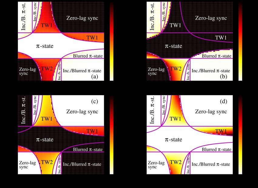
2

above include laser arrays [30, 31] and electrochemical os-                       III.    DIMENSIONAL REDUCTION
cillators [32, 33]. Furthermore, the balance between phase-
attraction and -repulsion has been recently shown to be a key         In the continuum limit N → ∞, we rewrite the original
factor in the regulation of circadian rhythms by pacemakers         Eq. (1) by omitting the sub-indexes as
cells in the suprachiasmatic nucleus (SCN) [34].
   Motivated by the aforementioned contributions, here we in-                            θ̇ = ω0 + KR sin(Θ − θ),                   (2)
vestigate the model in Ref. [24] of identical oscillators in the
absence of stochastic fluctuations acting on the frequencies.       where R and Θ are the “weighted” order parameter and the
We divide the oscillators into two subpopulations asymmet-          mean-field phase, respectively, defined by
rically coupled, and employ the theory by Ott and Antonsen                          Z Z
(OA) [35, 36] to obtain a reduced set of equations that de-                ReiΘ =         GrK,G eiψK,G P (K, G)dKdG.     (3)
scribes the evolution of the system. By studying the linear
stability of the reduced system, we analytically derive sev-        P (K, G) is the joint distribution of in- and out-coupling
eral conditions that delineate the transitions between synchro-     strengths; variables rK,G eiφK,G are the local order parameters
nized, incoherent, traveling-waves and π-states. Interestingly,     that quantify the synchrony within subpopulations:
we find the dynamics of the present model to be overall more
intricate than its stochastic version [24], with wider regions in
                                                                                                     Z
the parameter space exhibiting coexistence between different                zK,G = rK,G eiψK,G = ρ(θ, t|K, G)eiθ dθ,            (4)
synchronization patterns. As we shall see, simulations with
large populations of oscillators in general confirm with excel-     where ρ(θ, t|K, G) is the probability density function of ob-
lent agreement the predictions by the theory; for a small set       serving an oscillator with phase θ at time t for a given
of parameters, however, we report strong deviations from the        coupling pair (K, G). Henceforth we adopt the notation
dynamics yielded by the reduced system.                             ρ
                                                                    R K,G (θ, t) ≡ ρ(θ, t|K, G). The normalization condition
                                                                      π
                                                                         ρ
                                                                      −π K,G
                                                                               (θ, t)dθ = 1 leads to the following continuity equa-
                                                                    tion:

                          II.   MODEL                                   ∂ρK,G   ∂
                                                                              +    {ρK,G [ω0 + KR sin(Θ − θ)]} = 0.                 (5)
                                                                          ∂t    ∂θ
   Following Sonnenschein et al. [24], we study here the sys-       Next we expand the phase density ρK,G (θ, t) in a Fourier se-
tem made up of N identical Kuramoto oscillators whose equa-         ries and apply the ansatz by Ott and Antonsen [35, 36] to its
tions are given by                                                  coefficients to get
                                                                                              N
                                                                                                                         !
                             N
                          Ki X                                                        1      X
                                                                                                                n inθ
             θ̇i = ω0 +         Gj sin(θj − θi ),            (1)      ρK,G (θ, t) =      1+      [αK,G (ω0 , t)] e + c.c , (6)
                          N j=1                                                      2π      n=1

                                                                    where αK,G (t) ≡ α(K, G, t), and c.c. stands for the complex
where i = 1, ..., N , and ω0 is the natural frequency. Notice       conjugate. Substituting Eq. (6) into Eq. (5) yields
that, in contrast to Ref. [24], we do not consider identical os-
cillators under the influence of stochastic fluctuations in the                                       K 2
                                                                              α̇K,G + iω0 αK,G +       (α   R − R∗ ) = 0,           (7)
phase dynamics; instead, the only source of disorder is the                                           2 K,G
one inflicted by the coupling strengths. We henceforth refer to
parameters Ki and Gj as the in- and out-coupling strengths,         Inserting Eq. (5) into Eq. (4), we have that the local order
                                                                                                    ∗
respectively. As defined in Eq. (1), these couplings set the        parameters become zK,G = αK,G      . Hence, for a general dis-
interactions between the oscillators to be asymmetric (or di-       tribution of coupling strengths P (K, G), we get
rected): oscillator i contributes to the dynamics of neighbor-
                                                                              K
ing nodes with weight Gi , while the input arising from other       ṙK,G =             2
                                                                                (1 − rK,G   )hhG0 rK 0 ,G0 cos(ψK,G − ψK 0 ,G0 ii
oscillators is weighted by Ki . The first model by Hong and                   2
                                                                                    K              −1
Strogatz [17] is recovered when Gi = 1∀i in Eq. (1) (no out-        ψ̇K,G = ω0 − (rK,G + rK,G           )hhG0 rK 0 ,G0 sin(ψK 0 ,G0 − ψK,G )ii
coupling strengths), while the second model investigated by                         2
                                                                                                                                      (8)
the same authors [19] is obtained by symmetrizing the in-
                                                                                          P (K 0 , G0 )...dK 0 dG0 .
                                                                                     RR
                                                                    where hh...ii =
coupling strengths, i.e., Ki = 1∀i. Bifurcation conditions
                                                                       The boundaries of the asynchronous state (R = 0)
have been calculated recently for a stochastic system with a
                                                                    can be obtained straightforwardly for arbitrary distributions
coupling scheme similar to Eq. (1) [37]. Other similar forms
                                                                    P (K, G). By considering small perturbations δrK,G around
of the coupling setting of Eq. (1) have also been addressed re-
                                                                    the incoherent state rK,G = 0, and setting ψK,G = 0, without
cently in Refs. [15, 38], considering a phase frustration term
                                                                    loss of generality, we get from Eq. (8)
in the interaction function (Kuramoto-Sakaguchi model [39]),
and in populations of asymmetrically coupled Rössler oscilla-
                                                                                          ˙ K,G = K hhG0 δrK 0 ,G0 ii.
                                                                                         δr                                         (9)
tors [40].                                                                                        2
3
with the classical Kuramoto order parameter as:
1
r(t)eiΦ(t) = [r1 (t)eiψ1 (t) + r2 (t)eiψ2 (t) ] (13)
2
Note that r(t)eiΦ(t) in the above equation is different from
the “weighted” order parameter ReiΘ = 21 [r1 (t)G1 eiψ1 (t) +
r2 (t)G2 eiψ2 (t) ] [Eq. (3)], which can be larger than one.
Equations (12) are very similar to the set of equations for
identical oscillators under the influence stochastic fluctua-
tions obtained via Gaussian approximation [24, 29]. Actually,
the only difference between the reduced system obtained in
FIG. 1. Schematic illustration of a finite system composed of two 4
intertwined subpopulations. Oscillators belonging to subpopula- Ref. [24] and Eq. (12) is that the former exhibits terms r1,2
2
tion 1 (2) interact among themselves via couplings K1 G1 (K2 G2 ), instead of r1,2 in the equations for ṙ1,2 ; and terms propor-
while oscillators from different subpopulations interact asymmetri- −1 3 −1
tional to (r1,2 + r1,2 ) in place of (r1,2 + r1,2 ) in the equation
cally with effective couplings K1 G2 and K2 G1 , as depicted above.
for δ̇. Notice also that Eqs. (12) could be obtained via the
Watanabe-Strogatz theory [41, 42] under uniform distribution
of constants of motion (Ott-Antonsen manifold) [18, 36].
By multiplying the previous equation by G and averaging over
From Eqs. (12), we expect to observe the following sta-
the distribution P (K, G), we rewrite Eq. (9) in terms of a per-
tionary states for the two subpopulation system (see the illus-
turbation to the global order parameter δR = hhG0 δrK 0 ,G0 ii,
˙ = [hhKGii/2]δR, which leads to the critical condition tration in Fig. 2): (i) the classical incoherent state in which
δR r = r1,2 = 0; (ii) the perfectly synchronized state in which
r1,2 = 1 and δ = 0 (we denominate this state as “zero-lag
hhKGii = 0. (10) sync” state); (iii) partially synchronized states characterized
by r1,2 < 1 and δ = 0, and which we refer to as “blurred
Therefore, for hhKGii < 0, the oscillators remain incoherent, zero-lag sync” states; (iv) the so-called “π-state” for which the
while for hhKGii > 0 the incoherent state loses stability, and subpopulations are perfectly synchronized (r1,2 = 1), while
a partially synchronized state sets in. Notice that Eq. (10) remaining diametrically opposed in the phase space (δ = π),
is similar to the condition obtained in Ref. [24] for identical yielding, hence, a vanishing global synchronization (r = 0);
oscillators subjected to Gaussian noise. (v) “blurred“ π-states, in which at least one of the subpopu-
Let us consider now the case in which the oscilla- lations is partially synchronized (r1,2 < 1) and the peaks of
tors are coarse-grained into n intertwined subpopulations their phase distributions are separated by δ = π; and, finally,
1
Pnjoint distribution of couplings given by P (K, G) =
with (vi) the traveling-wave (TW) state [17, 24, 43] in which the
n q=1 δ[(K, G) − (Kq , Gq )]. Substituting the previous ex- subpopulations can be either partially or fully synchronized,
pression for P (K, G) into Eqs. (8) yields 0 < r1,2 ≤ 1, while keeping a constant phase-lag separa-
tion within 0 < δ < π. The interesting feature of this state
n
Kq X is that, in contrast to standard formulations of the Kuramoto
ṙq = − (1 − rq2 ) Gp rp cos(ψp − ψq )
2n model, the oscillators no longer rotate with a common fre-
p=1
(11) quency given by the frequency ω0 of the co-rotating frame–
n R
Kq X or ω̄ = ωg(ω)dω in the case of non-identical oscillators,
ψ̇q = ω0 − (rq + rq−1 ) Gp rp sin(ψp − ψq ).
2n where g(ω) is a frequency distribution [17, 43]–; instead, they
p=1
settle on a stationary new rhythm whose magnitude will also
depend on the coupling parameters. Deviations from the mean
In what follows we investigate a special case of the above
frequency ω̄ can be calculated either by the average (or mean-
system, namely, the setup of two intertwined subpopula-
ensemble) frequency
tions [24]. In this case, we have n = 2, and Eqs. (11) are
reduced to
N
1 X
K1 Ω= hθ̇j it , (14)
ṙ1 = (1 − r12 )[r1 G1 + r2 G2 cos δ], N j=1
4
K2
ṙ2 = (1 − r22 )[r2 G2 + r1 G1 cos δ], where h...it denotes a long-time average; or by the locking
4
sin δ frequency Θ̇, defined in Eq. (3) [see also Eq. (18)]. TW
(r1 + r1−1 )r2 K1 G2 + (r2 + r2−1 )r1 K2 G1 ,
δ̇ = − states typically appear in phase-oscillator systems when cer-
4
(12) tain symmetry patterns are broken in the model, such as by the
where we have defined the phase-lag δ = ψ1 −ψ2 . An illustra- presence of a phase frustration in the sine coupling term [39],
tion of a finite network with two intertwined subpopulations asymmetric coupling strength distributions [17, 18], or by nat-
can be seen in Fig. 1. We measure the global synchronization ural frequencies asymmetrically distributed [43].4
FIG. 2. Long-time profile on the complex unit circle of the states observed for a finite system [Eq. (1)] with two intertwined subpopulations
coupled as depicted in Fig. 1: (a) Incoherent state, (b) Zero-lag sync, (c) π-state, (d) TW1, (e) blurred zero-lag sync, and (f) blurred π-state.
Only in the TW1 state [panel (d)], the collective frequencies Θ̇ [Eq. (18)], Φ̇ [Eq. (13)] and Ω [Eq. (14)] are different from zero, and the
oscillators travel across all possible phase values in the co-rotating frame defined by the natural frequency. The configuration of the TW2 state
is obtained by interchanging sub-indexes and colors in panel (d).
IV. BIFURCATION ANALYSIS OF THE REDUCED Equation (16) corresponds to the solution of partially synchro-
SYSTEM WITH TWO SUBPOPULATIONS nized states with no separation between populations (even m)
and π-states (odd m), while Eq. (17) gives the condition for
For convenience, we adopt the following parametrization the existence of TW states. We can verify that TWs appear
for the couplings: only for 0 < δ < π by rewriting the equations for ψ̇1,2 to-
gether with Eq. (17) as:
∆K ∆G
K1,2 = K0 ± and G1,2 = G0 ± , (15)
2 2 r2 + r2−1
lim ψ̇1,2 = lim Θ̇ = ω0 − sin δ K2 G1 r1 . (18)
where K0 and G0 are the average in- and out-coupling t→∞ t→∞ 4
strengths, respectively; parameters ∆K and ∆G are defined Therefore, spontaneous drifts in the collective frequencies oc-
as the corresponding coupling mismatches. In our calcula- cur only for intermediate values of the phase-lag δ; otherwise,
tions we always consider positive mismatches (∆K, ∆G > for δ = mπ, oscillators rotate with collective frequencies
0). Therefore, if |K0 | < ∆K/2 or |G0 | < ∆G/2, half of the ψ̇1,2 = ω0 , which here is set to ω0 = 0.
couplings are positive (attractive) and half are negative (re- From the parametrization in Eq. (15), we realize the critical
pulsive). If one of these conditions is satisfied, we say that the conditions K1,2 = 0, or
oscillators interact via mixed couplings.
By setting δ̇ = 0, we uncover two possible fixed-point so- ∆K
lutions for phase-lag δ: K0 = ± . (19)
2
δ = mπ, m ∈ Z (16) When one of the above conditions holds, it follows that
0 = (r1 + r1−1 )r2 K1 G2 + (r2 + r2−1 )r1 K2 G1 . (17) one subpopulation is deprived of receiving inputs from other5
nodes (including from the same subpopulation), and its oscil- C. Zero-lag sync and partially synchronized states
lators have instead only out-couplings towards nodes external
to their subpopulation. Similarly, if one of the out-couplings For the zero-lag sync state, we linearize Eqs. (12) around
vanishes, G1,2 = 0, the corresponding subpopulation ceases r1,2 = 1 and δ = 0, and seek a zero eigenvalue of the re-
to influence the dynamics of the rest of the network and starts lated Jacobian matrix. By following this calculation, we find
acting only as link receiver. As we shall see, these conditions that the zero-lag sync state emerges for average in-coupling
play an important role in the phase diagram of Eq. (12). In the strengths given by
sequel, we calculate the coupling ranges in which the states
discussed in the previous section appear. ∆K ∆K∆G
K0 > max , , for G0 > 0;
2 4G0
(23)
∆K ∆K∆G
A. Incoherent state K0 < min − , , for G0 < 0.
2 4G0
The first critical condition of Eqs. (12) is given by the stabil- Next, by linearizing Eqs. (12) around an arbitrary partially
ity analysis of the incoherent state performed in the last sec- synchronized solution (r1 G1 = −r2 G2 and δ = 0), we find
tion. For the case of two subpopulations with P (K, G) = that such states, which we have denominated blurred zero-lag
1 1 sync states, must occur for parameters in the range
2 δ[(K, G) − (K1 , G1 )] + 2 δ[(K, G) − (K2 , G2 )], Eq. (10)
reads K1 G1 + K2 G2 = 0, and by solving it in terms of the
∆K∆G ∆G
average in-coupling strength we have K0 < , for |G0 | < . (24)
4G0 2
∆K∆G
K0 = − . (20) Any state that satisfies r1 G1 = −r2 G2 and δ = 0 is a fixed
4G0 point of Eqs. (12). From this we foresee that several par-
tially synchronized states should coexist in the region delim-
The above equation, therefore, delineates the boundary of the
ited by Eq. (24). As in the case of blurred π-states, blurred
incoherent state.
zero-lag sync solutions yield a single nonzero Jacobian eigen-
value, λ = K1 G1 (1 − r12 )/4 + K2 G2 (1 − r22 )/4; hence,
the latter states do not coexist with zero-lag sync nor with π-
B. π-states states, because in regions where r1,2 = 1 we have λ = 0,
and the blurred zero-lag sync states lose stability. Notice fur-
For the π-state, the fixed point solutions read r1,2 = 1 and ther that in order to r1 G1 = −r2 G2 be a physical solution,
δ = π. Linear stability reveals that the π-state is stable for out-couplings G1 and G2 must have opposite signs; thus, par-
average in-couplings given by tially synchronized states with δ = 0 are expected to appear
only in the presence of mixed-out coupling strengths, i.e., for
|G0 | < ∆G/2, as indicated in Eq. (24).
∆K ∆K ∆K∆G
− < K0 < min , , for G0 > 0;
2 2 4G0
(21)
∆K ∆K∆G ∆K D. Traveling waves
max − , < K0 < , for G0 < 0.
2 4G0 2
We now turn our attention to the stationary TW states. Nu-
The other state characterized by subpopulations diametri- merical results show us that two possible TW states are mani-
cally opposed is the blurred π-state, and its fixed points are fested by the system (12). In the first state, which we refer to
defined by r1 G1 = r2 G2 and δ = π. Linearizing the dy- as “TW1”, the first subpopulation remains fully synchronized
namics about this state, we find that the corresponding Jaco- (r1 = 1), whereas the second one exhibits partial synchroniza-
bian matrix has a single nonzero eigenvalue, λ = K1 G1 (1 − tion (r2 < 1). We label as “TW2” the opposite situation, i.e.,
r12 )/4 + K2 G2 (1 − r22 )/4. Hence, and because couplings G1 when r2 = 1 and r1 < 1. In both states we have 0 < δ < π
and G2 must have the same sign so that r1 G1 = r2 G2 is a and Ω > 0. By setting r1 = 1 in Eqs. (12), we find the fol-
physical solution, we have that blurred π-states appear when lowing fixed point solutions for r2 and δ:
∆K∆G ∆G r
K0 < , for |G0 | > . (22) K2 G1 G2
4G0 2 r2 = − and cos δ = − r2 . (25)
K2 G1 + 2K1 G2 G1
Thus, both π-states with fully synchronous subpopulations Since 0 < r2 < 1, we have that the solution of the TW1 exists
(r1,2 = 1) and with partial synchronization (r1,2 < 1) are for
yielded by systems described by Eqs. (12). Observe also that
r1 G1 = r2 G2 defines a one-parameter family of fixed points. − K1 G2 < K2 G1 < 0. (26)
Furthermore, from Eq. (22) we notice that incoherent and
blurred π-states may coexist in a large region of the param- By writing Eq. (26) in terms of the parametrization in Eq. (15)
eter space defined by coupling strengths G0 and K0 . and considering ∆K, ∆G > 0, we find that the regions with6
(a) (b)
(c) (d)
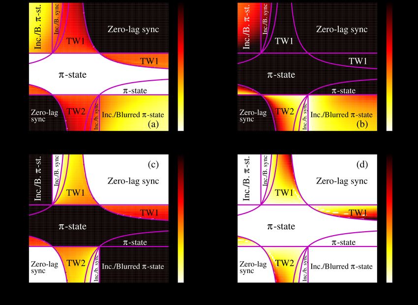
FIG. 3. Bifurcation diagram of the reduced system [Eq. (12)] for (a,b) ∆K = 8 and ∆G = 2; and (c,d) K0 = 3 and G0 = 2 . Zero-lag sync
corresponds to the perfectly synchronized state (r1,2 = 1 and δ = 0). “π-state” refers to the state in which r1,2 = 1 and phase-lag separation
δ = π. Similarly, blurred zero-lag and blurred π-states denote the states with r1,2 < 1 along with δ = 0 and δ = π, respectively. Traveling
wave states are characterized by r1 = 1, r2 < 1 (TW1), and r2 = 1, r1 < 1 (TW2). Both TW1 and TW2 exhibit Ω 6= 0 [Eq. (14)]. Solid
lines are obtained from Eqs. (20)-(24) and Eqs. (27)-(29). Dashed line in panels (a) and (c) depict the condition K0 ∆G − ∆KG0 = 0 for
which the couplings are symmetric, i.e., when the network connections are undirected. Panels (b) and (d) show zoomed-in regions of panels
(a) and (c), respectively.
TW1 are outlined by the following conditions: is stable:
2
∆K ∆K ∆G ∆G
< K0 < − , for − < G0 < 0;
2 8 G0 2
∆K∆G ∆K ∆G ∆K ∆K∆G ∆G
. (27) < K0 < , for 0 < G0 < .
4G0 2 2 2 4G0 2
(28)
The solutions for r1 and δ, and the critical conditions for the
TW2 state are obtained by interchanging indexes “1” and “2”
The linearization of Eqs. (12) about the fixed points of in Eqs. (25) and (26). By following the same procedure for
Eq. (25) also reveals a second region in which the TW1 state the corresponding TW2 solutions, one uncovers that this state7
appears for average in-coupling strengths given by thus, a fraction of the oscillators tends to align with the mean-
field (conformists oscillators), while the rest is repelled by it
∆K ∆K∆G ∆G (contrarians oscillators). As shown in Refs. [17, 18], the ab-
− < K0 < , for G0 < − ;
2 4G0 2 sence of out-coupling strengths does not impede the system
∆K∆G ∆K ∆G from reaching π-states and traveling-waves. Indeed, if we set
< K0 < − , for − < G0 < 0;
4G0 2 2 ∆G = 0 in Fig. 3(b) and follow the transitions along the K0 -
2 axis, we see that the system switches from TW1 to TW2 via
∆K ∆G ∆K ∆G
< K0 < − , for 0 < G0 < . crossing the central π-state area. In their follow-up study [19],
8 G0 2 2 the couplings were treated as properties of the links, that is,
(29)
the coupling terms were placed inside the summation over the
Alternatively, the conditions of the TW2 state [Eq. (29)] could
neighbors’ connections instead of outside as in Refs. [17, 18].
be obtained by letting (∆K, ∆G) → (−∆K, −∆G) in the
This coupling setting is equivalent to the model in Eq. (1) in
TW1 conditions [Eq. (27) and (28)].
the absence of in-coupling strength mismatches (∆K = 0).
Figure 3(a) depicts the bifurcation diagram outlined by the
Interestingly, despite the presence of mixed couplings, nei-
critical conditions in Eqs. (20)-(24) and Eqs. (27)-(29). As ther traveling waves nor π-states were detected, but rather
can be seen, for high values of both K0 and G0 , the dynam- only partially synchronized and incoherent states [19]. The
ics converges either to perfect synchronization or to incoher- fact that mixed out-couplings under no mismatch in the in-
ence/blurred π-state; for intermediate values, however, multi- couplings yield only a classical mean-field behavior is evident
ple regions of bistability appear. Interestingly, although sim- in Fig. 3, where we see that for ∆K = 0 the only possible
pler, the model in Eq. (1) exhibits a more complex dynamics state is zero-lag sync.
than its stochastic version [24]. By comparing the diagrams
of Fig. 3 with their counterparts in Ref. [24], we see that the
regions with coexistence between different states become pro-
portionally larger when noise is absent. A similar effect was V. SIMULATIONS
observed by Hong and Strogatz when comparing the findings
in Refs. [17, 18]. Let us now compare the results of the bifurcation analysis
By rewriting the critical couplings in Eqs. (20)-(24) and in the previous section with numerical simulations of the fi-
Eqs. (27)-(29) in terms of coupling mismatches, we derive the nite original dynamics [Eq. (1)]. Figure 4 shows the evolution
stability diagram spanned by the parameters ∆G and ∆K. of order parameters, phase-lag separation δ, and collective fre-
Similarly to what was verified in Ref. [24], the arrangement quencies, Ω and Θ̇, as a function of K0 for different choices of
of the transitions in Fig. 3 evidences some rules for the oc- G0 . All the simulations are performed by integrating Eqs. (1)
currence of the collective states manifested by the system with the Heun’s method with a time step dt = 0.005 and con-
(1). First, in order to observe π-states, mixed in-couplings sidering total number of oscillators N = 104 (see the caption
are required [see that the blue areas in Fig. 3(c) occur for of Fig. 4 for more details). For G0 = 0 [Fig. 4 (a), (d), and
∆K > 2K0 ]. States TW1 and TW2 emerge when either (g)] we observe that the system transitions from TW2 to π-
mixed in- or out-coupling exist, but never when both types state, and then subsequently to TW1, as correctly predicted
of couplings are mixed – in the latter case, only incoherence by the critical conditions depicted in the diagram of Fig. 3. In
and π-states are possible. Bistability of TWs and incoher- Fig. 4(b), we see that at K0 = −2 the subpopulations abruptly
ence with π-states appear when mixed in-coupling strengths synchronize as they switch from blurred π-states to π-state. A
exist, whereas we observe bistable regions TW/zero-lag sync similar discontinuous transition of the local order parameters
and TW/incoherence when only out-couplings are mixed. Fi- r1,2 was observed for similar parameter configurations in the
nally, we emphasize the importance of the directness in the stochastic version of the system (1) [24]. Abrupt transitions
network connections for the emergence of traveling waves. are also seen in Fig. 4(c), but this time as a consequence of
For K0 ∆G − ∆KG0 = 0, the coupling strengths connect- the transition from blurred zero-lag sync to TW2 state. In
ing the subpopulations become equal and the interaction is Fig. 4(c) we also observe irregular points in the “B. zero-lag
no longer asymmetric. By projecting this expression onto the sync” region. Those points correspond to partially synchro-
stability diagram (see the dashed lines in Fig. 3), we see that nized states and display such an irregular pattern because of
the symmetry condition does not intersect TW regions; there- the one-parameter family of solutions that exists in that re-
fore, asymmetric interactions are necessary for the emergence gion; specifically, different initial conditions drive the system
of such states. Nevertheless, as seen in Fig. 3, π-states are to different stationary states that satisfy r1 G1 = −r2 G2 . The
crossed by the line imposed by the symmetry relation, mean- solid branches in “B. zero-lag sync” area correspond to TW2
ing that asymmetric couplings are not required for the exis- solutions, which are also stable for K0 . −3.9 in Fig. 4(c)
tence of π-states. [see also Fig. 3(b)], but are not obtained numerically with the
The diagrams in Fig. 3 also allow us to reexamine the re- initial conditions used in Fig. 4. We shall return to this point
sults in Refs. [17–19] as particular cases of the present model. shortly.
As mentioned previously, in Refs. [17, 18], the authors stud- Notice in Fig. 4(g)-(i) that |Ω| ≤ |Θ̇|. The reason for this
ied Kuramoto oscillators subjected to attractive and repulsive resides in the fact that Ω is a microscopic average of the in-
in-couplings strengths (∆G = 0 in our notation). In that set- stantaneous frequencies hθ̇i i, while Θ̇ [and equivalently Φ̇ in
ting, the couplings are regarded as a property of the nodes; Eq. (13)] quantifies how fast the center of the bulk formed by8
Zero-lag B. zero-lag Zero-lag
TW2 -state TW1 Blurred -state -state TW1 sync sync TW2 -state TW1 sync
(a) (b) (c)
(d) (e) (f)
(g) (h) (i)
FIG. 4. Order parameters r1,2 , r, phase-lag δ, and collective frequencies Θ̇ [Eq. (18)] and Ω [Eq. (14)] for (a,d,h) G0 = 0, ∆K = 8, and
∆G = 2; (b,e,h) G0 = 2, ∆K = 8, and ∆G = 2; and (c,f,i) G0 = 2, ∆K = 3, and ∆K = 10 and ∆G = 2. Dots are obtained by
numerically integrating the original system [Eq. (1)] using the Heun’s method with N = 104 oscillators. For each coupling value K0 , the
quantities are averaged over t ∈ [500, 1500] with a time-step dt = 0.005. In all panels, initial conditions θi (t = 0) ∀i are randomly distributed
according to a uniform distribution between [−π, π]. Solid lines correspond to the analytic solutions obtained in Sec. IV.
entrained oscillators rotates. Therefore, oscillators that are not VI. ACCURACY OF THE OTT-ANTONSEN REDUCTION
locked with the mean-field contribute to the sum in Eq. (14)
with hθ̇i it ≈ 0, thus reducing the value of Ω in comparison Although we have observed a good agreement between
with its upper bound Θ̇. The latter frequency offers in the simulations and the theory for the states previously discussed,
present case the slight advantage of being calculated directly there are also dynamical patterns which seem not to be cap-
from the solutions in Eq. (18). Analogously, Ω can be es- tured by the OA reduction. Figure 6 shows an example: there
timated analytically
R π R R(not shown here) through the ensemble we observe a set of points with Θ̇ = 0 in the TW2 area, i.e., a
average Ω = −π θ̇ρ(θ, t|K, G)dKdGdθ. region where one would expect stationary states with Θ̇ 6= 0.
By inspecting the temporal trajectories of the local order pa-
To conclude this section, in Fig. 5 we compare the theoret- rameters r1,2 in Fig. 7, we see that such states do have a dif-
ical results with simulations considering coupling parameters ferent nature from traveling waves. The trajectories in Figs. 7
over a G0 × K0 grid. Our goal with this approach is to inspect actually resemble breathing chimera states [44] in which one
for a larger set of parameters whether the stability analysis subpopulation remains fully locked, while the other exhibits
performed in the previous section correctly predicts the stabil- an oscillating synchrony. In the figure, we compare the time
ity regions shown in Fig. 3. For each coupling pair (G0 , K0 ), evolution of the original model (1) with the numerical inte-
Eqs. (1) are integrated numerically, and the global variables gration of the reduced system [Eq. (12)] using the same ini-
are averaged over t ∈ [500, 1500] with a time step dt = 0.005. tial conditions. As it is seen, while the finite subpopulation
As can be seen in Fig. 5, the boundaries of the collective states 1 shows oscillating synchrony, the solution provided by the
are predicted very accurately by the theory. Seeking to verify theory converges to a constant value. Although chimera states
the bistable behavior of the model, in Fig. 6 we show sim- have been studied extensively with the OA reduction, Figs. 6
ulations results for a zoomed region of the space in Fig. 5 and 7 suggest that such solutions in the present model might
considering different initial conditions: in Fig. 6(a), phases θi lie outside the OA manifold. Interestingly, Refs. [17, 18, 24]
are initiated with values distributed uniformly at random be- did not report solutions akin to the ones shown in Fig. 7.
tween [−π, π]. Initial conditions were chosen differently for
Fig. 6(b); specifically, for each point in the grid G0 × K0 , the
phases of populations 1 and 2 were chosen from Gaussian dis-
tributions with standard deviation σ = 2, and means θ1 and VII. CONCLUSION
θ2 , which were taken uniformly at random between [−π, π].
By initiating the oscillators in this way, we observe in Fig. 6 In this paper we have studied a variant of the Kuramoto
that the system converges to TW2 in the region where this model in which identical oscillators are coupled via in-
state was predicted to coexist with partial synchronization. and out-coupling strengths, which in turn can have positive9 FIG. 5. Comparison between simulations (colormaps) and theory (solid lines). (a) Total order parameter r; (b) local order parameter r1 of subpopulation 1; (c) phase-lag δ measuring the separation between the two subpopulations; and (d) average frequency Ω [Eq. (14)]. For each pair of coupling (G0 , K0 ), Eqs. (1) are evolved numerically with the Heun’s method considering N = 104 oscillators and with integration time step dt = 0.005. The long-time behavior of each parameter is quantified by averaging the trajectories over t ∈ [500, 1000]. For all (G0 , K0 ), the initial phases θi (t = 0) are drawn uniformly at random over the interval [−π, π]. Coupling mismatch parameters: ∆K = 8 and ∆G = 2. and negative values. Similarly to the setting considered in states uncovered (which may consist of either perfectly or par- Ref. [24], heterogeneity in the interactions was introduced tially synchronized subpopulations), and in the observation by dividing the oscillators into two mutually coupled sub- of wider regions in the parameter space displaying bistabil- populations (each one characterized by a distinct pair of cou- ity. These findings for the seemingly simpler system are in plings), so that connections within the same subpopulation re- line with previous studies [17, 18] comparing the dynamics main symmetric, while connections between subpopulations of identical oscillators with that of non-identical ones. [Al- are asymmetric. In the infinite size limit, we applied the though the system in Eq. (1) and the one of Ref. [24] are theory by Ott and Antonsen [35] to obtain a reduced set of both models of identical oscillators, the inclusion of Gaussian equations. With the reduced description of the original sys- white noise yields equivalent phenomenology–with respect to tem, we performed a thorough bifurcation analysis whereby the linearized dynamics–to the case of phase oscillators with a rich dynamical behavior was revealed. We showed that natural frequencies drawn from Lorentzian distributions; see the present system exhibits different types of π-states and the discussion in Ref. [45].] traveling-waves, along with classical incoherent and partially Despite the excellent agreement between simulations and synchronized states. Though the transitions among these theory, for a small set of parameter combinations we veri- states bear some similarity to those uncovered for the model fied dynamical states which turned out not to be reproduced with Gaussian white noise in Ref. [24], we have found that by the reduced system. As discussed in Sec. VI, we veri- our model exhibits a more intricate long-term dynamics than fied vanishing values for the temporal average of the mean- that of observed for its noisy version. The reason for this con- field frequency for couplings inscribed in a TW region. By clusion resides in the different types of π- and zero-lag sync visualizing the time-series of such unanticipated states, we
10

                                                                                   (a)

                                                                                   (b)

                                                                                   (c)

                                                                         FIG. 7. Temporal evolution of (a) local order parameters r1,2 , (b)
FIG. 6. Comparison between simulations (colormaps) and theory            phase-lag δ, and (c) locking frequency Θ̇ [Eq. (18)]. Solid lines
(solid lines) for different sets of initial conditions: (a) θi (t = 0)   are obtained from simulations, while dashed lines correspond to the
randomly chosen from the uniform distribution [−π, π] (same as in        results yielded by the numerical integration of the reduced system
Fig. 5); (b) for each coupling pair (G0 , K0 ) the initial phases of     [Eq. (12)]. In panel (a) the solid and dashed lines of r2 overlap each
subpopulation 1 and 2 were drawn from Gaussian distributions with        other at r2 = 1. Average in- and out-coupling strengths are taken
standard deviation σ = 2, and means θ1 and θ2 , respectively, which      from the “+” point in Fig. 6(b), that is, (G0 , K0 ) = (−0.5, −5.95).
were chosen uniformly at random between [−π, π]. The “+” marks           Other parameters: N = 104 oscillators, ∆K = 8, ∆G = 2, and
a point in the diagram for which the behavior observed in the simu-      dt = 0.005.
lation departs from the dynamics predicted by the theory. Figure 7
shows the temporal evolution of the collective variables at the “+”
point depicted in panel (b). Other parameters: N = 104 , ∆K = 8          perturbations that may drive the system away from the man-
and ∆G = 2. In both panels the resolution of the grid is 100 × 100       ifold contemplated by the OA ansatz, thus generating unex-
couplings. Integration was performed with the Heun’s method using        pected results such as the ones discussed in Sec. VI. Another
time step dt = 0.005.                                                    deviation from the theory was observed in the appearance of
                                                                         zero-lag sync and π-states over a region in the parameter space
                                                                         initially believed to manifest traveling-waves solely [see Fig. 4
found that one local parameter evolved with an oscillatory dy-           (c)]. Future works should further investigate the emergence of
namics akin to breathing chimera states [44], in sharp con-              chimeras and other states with respect to perturbations off the
trast to the evolution predicted by our calculations for the             OA manifold for populations of identical oscillators coupled
same parameters and initial conditions. It is worth noting,              asymmetrically.
nonetheless, that disagreements of this nature are somewhat                 As mentioned in the introduction, there are many systems
expected to occur: for the identical frequencies case there ex-          whose dynamics can be modeled by phase oscillators inter-
ists a one-parameter family of invariant manifolds (of which             acting via positive and negative couplings. Our results can
the OA-manifold is a special solution) that are neutrally stable         thereby serve as a guide in the search for clustered states
with respect to perturbations in directions transverse to them-          in different contexts. For instance, as shown in Ref. [34],
selves [36, 42, 46, 47]. Hence, there could be certain types of          phase-attraction or phase-repulsion alone cannot account for
11 FIG. 8. Comparison between simulations (colormaps) and theory (solid lines). (a) Total order parameter r; (b) local order parameter r1 of subpopulation 1; (c) phase-lag δ measuring the separation between the two subpopulations; and (d) average frequency Ω [Eq. (14)]. For each pair of coupling (G0 , K0 ), Eqs. (1) are integrated numerically with the Heun’s method considering N = 104 oscillators and with integration time step dt = 0.005. The long-time behavior of each parameter is quantified by averaging the trajectories over t ∈ [500, 1000]. For all coupling pairs (G0 , K0 ), Eqs. (1) were initiated with the exact same configuration for θi (t = 0): phases in subpopulation 1 were randomly chosen from a Gaussian distribution with mean θ1 ' 0.17 and standard deviation σ1 ' 0.85, yielding r1 (t = 0) ' 0.69; phases of subpopulation 2 were also Gaussian distributed, but with mean θ2 ' 1.09 and standard deviation σ2 ' 1.053, yielding r2 (t = 0) ' 0.57. Coupling mismatch parameters: ∆K = 8 and ∆G = 2. G0 × K0 grid resolution: 100 × 100 couplings. the regulation of circadian rhythms; a phase model incorpo- of the dynamical transitions reported here may be obtained rating mixed couplings linked asymmetrically, on the other in populations of chemical [52, 53] and optical arrays [54], hand, does reproduce the outcome of experiments with neu- which are experimental setups that have been shown to re- ronal networks of the suprachiasmatic nucleus (SCN). There- produce chimeras and other dynamical states found in phase fore, system (1) with two intertwined subpopulations may be oscillator models. a suitable model to describe the synchronization between the dorsal and ventral subregions of the SCN [34]. Finally, there are a number of potentially relevant exten- sions for the present model: given the non-trivial behavior ACKNOWLEDGMENTS uncovered here, it would be interesting, for instance, to inves- tigate more than two coupled populations, as well as to study The author thanks Bernard Sonnenschein, Chen Chris the effect of attractive and repulsive interactions on the col- Gong, Deniz Eroglu, Paul Schultz, Vinicius Sciuti, and Bruno lective dynamics of oscillators with higher-order harmonics Messias for useful conversations. This research was funded in the coupling function [48, 49]. One could also consider os- by FAPESP (Grant No. 2016/23827-6) and carried out using cillators coupled on structures that allow interactions beyond the computational resources of the Center for Mathematical the classical pairwise, such as hypergraphs [50] and simpli- Sciences Applied to Industry (CeMEAI) funded by FAPESP cial complexes [51]. On the experimental domain, realizations (Grant No. 2013/07375-0).
12

              Appendix A: Supplementary diagram                          r1 = 1 in Fig. 8(b)]. In addition to the bistability between
                                                                         TWs and blurred zero-lag sync states confirmed in Sec. VI,
   In this section we recalculate the diagrams of Fig. 5 by ini-         another significant difference between Fig. 5 and Fig. 8 lies
tiating the oscillators differently than in Sec. V. Specifically,        in the “Incoherence/Blurred π-state” areas: in Fig. 5 these re-
in Fig. 8 we choose the phases of each subpopulation to be               gions exhibit small values for the order parameters (a conse-
distributed according to distinct Gaussian distributions whose           quence of choosing the initial conditions uniformly at random
peaks are separated by a phase-lag (see the caption of Fig. 8            between [−π, π]), along with δ = π; in Fig. 8, on the other
for details). Comparing Fig. 5 with Fig. 8 we see that a blurred         hand, we observe higher values for r1 , thus confirming that
π-state region in the former is converted into a π-state area in         multiple local synchronization levels are possible in those re-
the latter [notice the regions with r1 = 0 in Fig. 5(b) and              gions as revealed by the analysis in Sec. IV.

 [1] Juan A Acebrón, Luis L Bonilla, Conrad J Pérez Vicente, Félix         (Europhysics Letters) 72, 190 (2005).
     Ritort, and Renato Spigler, “The Kuramoto model: A simple           [17] Hyunsuk Hong and Steven H Strogatz, “Kuramoto model of
     paradigm for synchronization phenomena,” Reviews of Modern               coupled oscillators with positive and negative coupling param-
     Physics 77, 137 (2005).                                                  eters: an example of conformist and contrarian oscillators,”
 [2] Francisco A Rodrigues, Thomas K DM Peron, Peng Ji, and                   Physical Review Letters 106, 054102 (2011).
     Jürgen Kurths, “The Kuramoto model in complex networks,”           [18] Hyunsuk Hong and Steven H Strogatz, “Conformists and con-
     Physics Reports 610, 1–98 (2016).                                        trarians in a Kuramoto model with identical natural frequen-
 [3] Alex Arenas, Albert Dı́az-Guilera, Jurgen Kurths, Yamir                  cies,” Physical Review E 84, 046202 (2011).
     Moreno, and Changsong Zhou, “Synchronization in complex             [19] Hyunsuk Hong and Steven H Strogatz, “Mean-field behavior in
     networks,” Physics Reports 469, 93–153 (2008).                           coupled oscillators with attractive and repulsive interactions,”
 [4] Arthur T Winfree, “Biological rhythms and the behavior of pop-           Physical Review E 85, 056210 (2012).
     ulations of coupled oscillators,” Journal of Theoretical Biology    [20] Ernest Montbrió and Diego Pazó, “Collective synchronization
     16, 15–42 (1967).                                                        in the presence of reactive coupling and shear diversity,” Phys-
 [5] Georg Heinrich, Max Ludwig, Jiang Qian, Björn Kubala, and               ical Review E 84, 046206 (2011).
     Florian Marquardt, “Collective dynamics in optomechanical ar-       [21] Dmytro Iatsenko, Spase Petkoski, PVE McClintock, and A Ste-
     rays,” Physical Review Letters 107, 043603 (2011).                       fanovska, “Stationary and traveling wave states of the Ku-
 [6] Kurt Wiesenfeld, Pere Colet, and Steven H Strogatz, “Syn-                ramoto model with an arbitrary distribution of frequencies
     chronization transitions in a disordered Josephson series array,”        and coupling strengths,” Physical Review Letters 110, 064101
     Physical Review Letters 76, 404 (1996).                                  (2013).
 [7] István Z Kiss, Yumei Zhai, and John L Hudson, “Emerging            [22] Hyunsuk Hong, “Periodic synchronization and chimera in con-
     coherence in a population of chemical oscillators,” Science 296,         formist and contrarian oscillators,” Physical Review E 89,
     1676–1678 (2002).                                                        062924 (2014).
 [8] Florian Dörfler and Francesco Bullo, “Synchronization in com-      [23] Isabel M Kloumann, Ian M Lizarraga, and Steven H Strogatz,
     plex networks of phase oscillators: A survey,” Automatica 50,            “Phase diagram for the Kuramoto model with van hemmen in-
     1539–1564 (2014).                                                        teractions,” Physical Review E 89, 012904 (2014).
 [9] Shir Shahal, Ateret Wurzberg, Inbar Sibony, Hamootal Duadi,         [24] Bernard Sonnenschein, Thomas K DM Peron, Francisco A Ro-
     Elad Shniderman, Daniel Weymouth, Nir Davidson, and Moti                 drigues, Jürgen Kurths, and Lutz Schimansky-Geier, “Col-
     Fridman, “Synchronization of complex human networks,” Na-                lective dynamics in two populations of noisy oscillators with
     ture Communications 11, 1–10 (2020).                                     asymmetric interactions,” Physical Review E 91, 062910
[10] Hiroaki Daido, “Quasientrainment and slow relaxation in a pop-           (2015).
     ulation of oscillators with random and frustrated interactions,”    [25] Bertrand Ottino-Löffler and Steven H Strogatz, “Volcano tran-
     Physical Review Letters 68, 1073 (1992).                                 sition in a solvable model of frustrated oscillators,” Physical
[11] LL Bonilla, CJ Pérez Vicente, and JM Rubi, “Glassy synchro-             Review Letters 120, 264102 (2018).
     nization in a population of coupled oscillators,” Journal of Sta-   [26] Jinha Park and B Kahng, “Metastable state en route to traveling-
     tistical Physics 70, 921–937 (1993).                                     wave synchronization state,” Physical Review E 97, 020203
[12] JC Stiller and G Radons, “Dynamics of nonlinear oscillators              (2018).
     with random interactions,” Physical Review E 58, 1789 (1998).       [27] Dustin Anderson, Ari Tenzer, Gilad Barlev, Michelle Girvan,
[13] Hiroaki Daido, “Algebraic relaxation of an order parameter in            Thomas M Antonsen, and Edward Ott, “Multiscale dynam-
     randomly coupled limit-cycle oscillators,” Physical Review E             ics in communities of phase oscillators,” Chaos: An Interdisci-
     61, 2145 (2000).                                                         plinary Journal of Nonlinear Science 22, 013102 (2012).
[14] JC Stiller and G Radons, “Self-averaging of an order parameter      [28] Jinha Park and B Kahng, “Competing synchronization on ran-
     in randomly coupled limit-cycle oscillators,” Physical Review            dom networks,” Journal of Statistical Mechanics: Theory and
     E 61, 2148 (2000).                                                       Experiment 2020, 073407 (2020).
[15] Dima Iatsenko, Peter VE McClintock, and Aneta Stefanovska,          [29] Bernard Sonnenschein and Lutz Schimansky-Geier, “Approxi-
     “Glassy states and super-relaxation in populations of coupled            mate solution to the stochastic Kuramoto model,” Physical Re-
     phase oscillators,” Nature communications 5, 4118 (2014).                view E 88, 052111 (2013).
[16] Damián H Zanette, “Synchronization and frustration in oscil-       [30] Chene Tradonsky, Micha Nixon, Eitan Ronen, Vishwa Pal, Ro-
     lator networks with attractive and repulsive interactions,” EPL          nen Chriki, Asher A Friesem, and Nir Davidson, “Conversion
13
of out-of-phase to in-phase order in coupled laser arrays with Physical Review Letters 101, 264103 (2008).
second harmonics,” Photonics Research 3, 77–81 (2015). [43] Spase Petkoski, Dmytro Iatsenko, Lasko Basnarkov, and Aneta
[31] Vishwa Pal, Simon Mahler, Chene Tradonsky, Asher A Stefanovska, “Mean-field and mean-ensemble frequencies of a
Friesem, and Nir Davidson, “Rapid fair sampling of the x y system of coupled oscillators,” Physical Review E 87, 032908
spin hamiltonian with a laser simulator,” Physical Review Re- (2013).
search 2, 033008 (2020). [44] Daniel M Abrams, Rennie Mirollo, Steven H Strogatz, and
[32] Hiroshi Kori, István Z Kiss, Swati Jain, and John L Hudson, Daniel A Wiley, “Solvable model for chimera states of coupled
“Partial synchronization of relaxation oscillators with repulsive oscillators,” Physical Review Letters 101, 084103 (2008).
coupling in autocatalytic integrate-and-fire model and electro- [45] Bastian Pietras, Nicolás Deschle, and Andreas Daffertshofer,
chemical experiments,” Chaos: An Interdisciplinary Journal of “Equivalence of coupled networks and networks with multi-
Nonlinear Science 28, 045111 (2018). modal frequency distributions: Conditions for the bimodal and
[33] Michael Sebek and István Z Kiss, “Plasticity facilitates pattern trimodal case,” Physical Review E 94, 052211 (2016).
selection of networks of chemical oscillations,” Chaos: An In- [46] Erik A Martens, “Bistable chimera attractors on a triangu-
terdisciplinary Journal of Nonlinear Science 29, 083117 (2019). lar network of oscillator populations,” Physical Review E 82,
[34] Jihwan Myung, Sungho Hong, Daniel DeWoskin, Erik 016216 (2010).
De Schutter, Daniel B Forger, and Toru Takumi, “Gaba- [47] Seth A Marvel, Renato E Mirollo, and Steven H Strogatz,
mediated repulsive coupling between circadian clock neurons “Identical phase oscillators with global sinusoidal coupling
in the scn encodes seasonal time,” Proceedings of the National evolve by möbius group action,” Chaos: An Interdisciplinary
Academy of Sciences 112, E3920–E3929 (2015). Journal of Nonlinear Science 19, 043104 (2009).
[35] Edward Ott and Thomas M Antonsen, “Low dimensional be- [48] Chen Chris Gong and Arkady Pikovsky, “Low-dimensional
havior of large systems of globally coupled oscillators,” Chaos: dynamics for higher-order harmonic, globally coupled phase-
An Interdisciplinary Journal of Nonlinear Science 18, 037113 oscillator ensembles,” Physical Review E 100, 062210 (2019).
(2008). [49] Per Sebastian Skardal and Alex Arenas, “Abrupt desynchro-
[36] Arkady Pikovsky and Michael Rosenblum, “Dynamics of glob- nization and extensive multistability in globally coupled oscil-
ally coupled oscillators: Progress and perspectives,” Chaos: lator simplexes,” Physical Review Letters 122, 248301 (2019).
An Interdisciplinary Journal of Nonlinear Science 25, 097616 [50] Guilherme Ferraz de Arruda, Giovanni Petri, and Yamir
(2015). Moreno, “Social contagion models on hypergraphs,” Physical
[37] JM Meylahn, “Two-community noisy Kuramoto model,” Non- Review Research 2, 023032 (2020).
linearity 33, 1847 (2020). [51] Ana P Millán, Joaquı́n J Torres, and Ginestra Bianconi, “Ex-
[38] Vladimir Vlasov, Elbert EN Macau, and Arkady Pikovsky, plosive higher-order Kuramoto dynamics on simplicial com-
“Synchronization of oscillators in a Kuramoto-type model with plexes,” Physical Review Letters 124, 218301 (2020).
generic coupling,” Chaos: An Interdisciplinary Journal of Non- [52] Jan Frederik Totz, Julian Rode, Mark R Tinsley, Kenneth
linear Science 24, 023120 (2014). Showalter, and Harald Engel, “Spiral wave chimera states
[39] Hidetsugu Sakaguchi and Yoshiki Kuramoto, “A soluble active in large populations of coupled chemical oscillators,” Nature
rotater model showing phase transitions via mutual entertain- Physics 14, 282–285 (2018).
ment,” Progress of Theoretical Physics 76, 576–581 (1986). [53] Dumitru Călugăru, Jan Frederik Totz, Erik A Martens, and
[40] Thomas K DM Peron, Jürgen Kurths, Francisco A Rodrigues, Harald Engel, “First-order synchronization transition in a large
Lutz Schimansky-Geier, and Bernard Sonnenschein, “Travel- population of strongly coupled relaxation oscillators,” Science
ing phase waves in asymmetric networks of noisy chaotic at- advances 6, eabb2637 (2020).
tractors,” Physical Review E 94, 042210 (2016). [54] Aaron M Hagerstrom, Thomas E Murphy, Rajarshi Roy, Philipp
[41] Shinya Watanabe and Steven H Strogatz, “Constants of motion Hövel, Iryna Omelchenko, and Eckehard Schöll, “Experimen-
for superconducting josephson arrays,” Physica D: Nonlinear tal observation of chimeras in coupled-map lattices,” Nature
Phenomena 74, 197–253 (1994). Physics 8, 658–661 (2012).
[42] Arkady Pikovsky and Michael Rosenblum, “Partially integrable
dynamics of hierarchical populations of coupled oscillators,”You can also read