Effects of magnetic bypass on performance of distribution transformers
←
→
Page content transcription
If your browser does not render page correctly, please read the page content below
DF

Effects of magnetic bypass on perfor-
mance of distribution transformers
Master’s thesis in Electric Power Engineering

MUNEEB BASHIR CHOUDHRY
MOHSIN UL HASSAN SYED

Department of Electric Power Engineering
C HALMERS U NIVERSITY OF T ECHNOLOGY
Gothenburg, Sweden 2019
Master’s thesis

      Effects of Magnetic Bypass on
Performance of Distribution Transformers

        MUNEEB BASHIR CHOUDHRY
          MOHSIN UL HASSAN SYED

                               DF

          Department of Electric Engineering
        Division of Electric Power Engineering
       Chalmers University of Technology
               Gothenburg, Sweden 2019
Effects of Magnetic Bypass on performance of Distribution Transformers.
MUNEEB BASHIR CHOUDHRY , MOHSIN UL HASSAN SYED

© MUNEEB BASHIR CHOUDHRY, MOHSIN UL HASSAN SYED 2019.

Supervisor: Thomas Türk, Transformer Cage Core AB
Examiner: Yuiry Serdyuk, Department of Electric Engineering, Chalmers University
of Technology

Master’s Thesis
Department of Electric Engineering
Division of Electric Power Engineering
Chalmers University of Technology
SE-412 96 Gothenburg
Telephone +46 31 772 1000

Cover: vector representation of reduction of loss angle with bypass.

Typeset in LATEX, template by David Frisk
Gothenburg, Sweden 2019

iv
Abstract
As the demand for electricity is increasing, the requirement for number of electrical
appliances is also increasing. With this increase in number of appliances, the perfor-
mance criteria for such appliances is also becoming less tolerant. One such important
appliance in the power system is distribution transformer. Significant contribution
of losses in a distribution transformer is incurred because of no-load losses, if such
a transformer is operated at no-load for longer duration then cumulative no-load
losses will have a high percentage of total losses. The new EU Commission regula-
tions recommend a further 10 % decrease in the no-load losses by the year 2021.

In this thesis, a prototype of power electronics based active core is developed for
a prototype hexa-Core transformer. Since the shape of flux in the winding is sinu-
soidal and so it follows a hysteresis curve, where magnetic domains are aligned in
both of the cycles. The aim was to assist in this change in domain alignment and as
a result excitation current from the supply can be reduced, decreasing no-load losses.

The response of this active core was evaluated with fixed DC value for a number of
excitation levels in the main core and with fixed excitation in the main core and a
number of DC values. Single step grain oriented magnetic bypasses were installed
in the core which resulted in the loss reduction of 15% to 19.5% in the main core.
This reduction of losses in the core was influenced by the decrease of magnetic flux
in the core rings. Furthermore these magnetic bypasses were excited to obtain fur-
ther loss reduction in the core. This resulted in a further decrease in power loss of
approximately 5% depending on the transformer’s main excitation and DC value.
Further to determine the optimum position for the secondary excitation from DC
source the pulse width and firing delay was evaluated.

Another type of wound core transformer the so called evans-core transformer was
also tested. The transformer showed similar behaviour to that of hexa-core. Dif-
ferent bypass strategies were also evaluated and a decrease in excitation losses was
achieved with these bypass strategies.

Keywords: Hexa-core Transformer, Transformer losses, Magnetic Bypass, Active
Core Control, Evan’s Core, Hexa-core, Single step bypass, Evans core.

                                                                                    v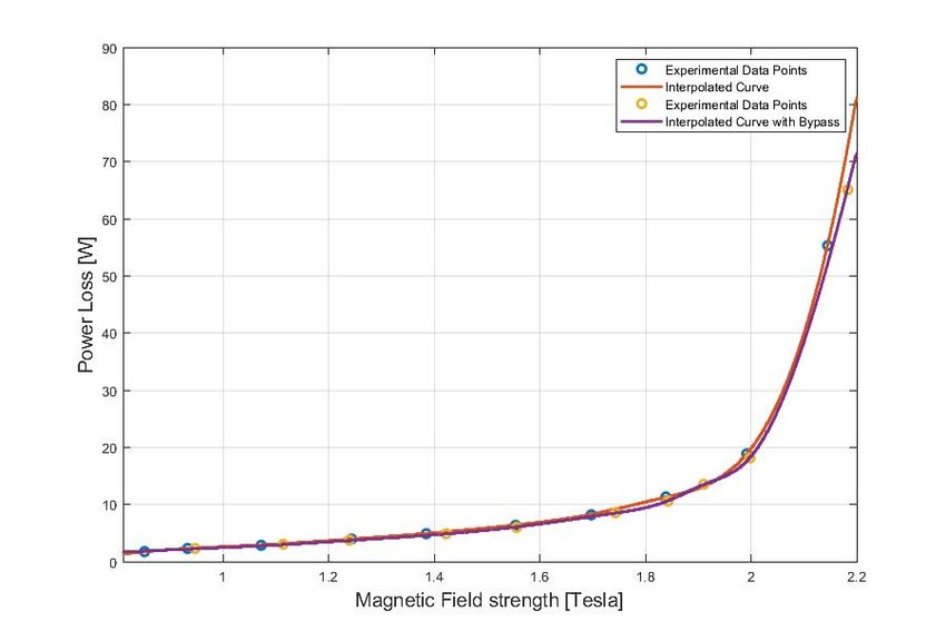
Acronyms
CSA     Cross-sectional area
EGO-1   Evans-core grain oriented bypass 1
EGO-2   Evans-core grain oriented bypass 2
EGO-3   Evans-core grain oriented bypass 3
φa      Flux in bypass
φA      Flux in leg A
φB      Flux in leg B
φC      Flux in leg C
A1      Inner Core ring 1
A2      Inner Core ring 2
α       Loss Angle
SPWM    Sinusoidal Pulse Width Modulation
WA      Winding on leg A of Evan’s core transformer
WB      Winding on leg B of Evan’s core transformer
WC      Winding on leg C of Evan’s core transformer
W1      Winding on leg 1 of Hexa-core transformer
W2      Winding on leg 2 of Hexa-core transformer
W3      Winding on leg 3 of Hexa-core transformer
ya      yoke between winding 1 and winding 2
yb      yoke between winding 2 and winding 3
yc      yoke between winding 1 and winding 3

                                                      vii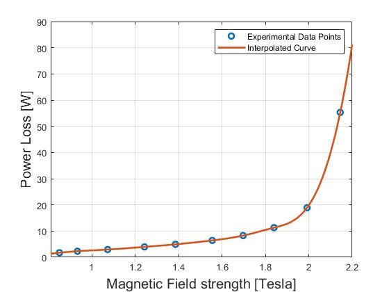
Acknowledgements
Authors would like to thanks ALLAH Almighty for giving us the will and strength
to complete this thesis work. Authors would also like to thank and pay sincere grati-
tude to Yuiry Serdyuk, supervisor and examiner of this project, for his guidance and
great support throughout the thesis work. His motivation, dedication and exper-
tise has helped us in achieving this goal and successfully completing our thesis work.

Authors would also acknowledge the efforts of Thomas Türk, supervisor at Trans-
former Cage Core AB and would also like to thank him for his motivation and
guidance towards this project work. His ideas has helped us throughout the thesis
work.

Authors would also like to express their sincere gratitude to everyone at the Divi-
sion of Electric Power Engineering for their help and guidance, esp. Haider Ali and
Douglas Nilsson, in completing this work.

Authors would also like to thank their families and friends for their love and support
throughout the whole studies.

                              Muneeb Bashir Choudhry, Gothenburg, October 2019
                                Mohsin Ul Hassan Syed, Gothenburg, October 2019

                                                                                    ix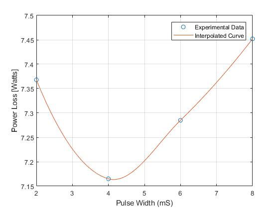
Contents

List of Figures                                                                                                            xiii

List of Tables                                                                                                             xv

1 Introduction                                                                                                               1
  1.1 Background . . . . . . . . . .     . . . . . . . .           .   .   .   .   .   .   .   .   .   .   .   .   .   .     1
  1.2 Problem description . . . . . .    . . . . . . . .           .   .   .   .   .   .   .   .   .   .   .   .   .   .     1
  1.3 Aim . . . . . . . . . . . . . .    . . . . . . . .           .   .   .   .   .   .   .   .   .   .   .   .   .   .     2
  1.4 Scope . . . . . . . . . . . . .    . . . . . . . .           .   .   .   .   .   .   .   .   .   .   .   .   .   .     2
  1.5 Limitations . . . . . . . . . .    . . . . . . . .           .   .   .   .   .   .   .   .   .   .   .   .   .   .     2
  1.6 Ethics and sustainable aspects     of the project            .   .   .   .   .   .   .   .   .   .   .   .   .   .     2

2 Transformer                                                                                                                3
  2.1 Working principle of transformer .       .   .   .   .   .   .   .   .   .   .   .   .   .   .   .   .   .   .   .     3
  2.2 Transformer Core & Material . . .        .   .   .   .   .   .   .   .   .   .   .   .   .   .   .   .   .   .   .     5
      2.2.1 Hexa-core transformer . . .        .   .   .   .   .   .   .   .   .   .   .   .   .   .   .   .   .   .   .     5
      2.2.2 Evans-core transformer . . .       .   .   .   .   .   .   .   .   .   .   .   .   .   .   .   .   .   .   .     6
      2.2.3 Ferromagnetic material . . .       .   .   .   .   .   .   .   .   .   .   .   .   .   .   .   .   .   .   .     6
  2.3 Losses in transformer . . . . . . . .    .   .   .   .   .   .   .   .   .   .   .   .   .   .   .   .   .   .   .     7
      2.3.1 Iron core losses . . . . . . .     .   .   .   .   .   .   .   .   .   .   .   .   .   .   .   .   .   .   .     7
             2.3.1.1 Eddy current losses       .   .   .   .   .   .   .   .   .   .   .   .   .   .   .   .   .   .   .     7
             2.3.1.2 Hysteresis losses .       .   .   .   .   .   .   .   .   .   .   .   .   .   .   .   .   .   .   .     8
      2.3.2 Copper losses . . . . . . . .      .   .   .   .   .   .   .   .   .   .   .   .   .   .   .   .   .   .   .     9
      2.3.3 Stray and Dielectric losses .      .   .   .   .   .   .   .   .   .   .   .   .   .   .   .   .   .   .   .     9

3 Bypass                                                                                                                    11
  3.1 Types    of Bypass configuration for Hexa-Core . . . . . . . .                               .   .   .   .   .   .    11
      3.1.1    Single step . . . . . . . . . . . . . . . . . . . . . . .                           .   .   .   .   .   .    11
      3.1.2    Two steps . . . . . . . . . . . . . . . . . . . . . . .                             .   .   .   .   .   .    11
      3.1.3    Three steps . . . . . . . . . . . . . . . . . . . . . .                             .   .   .   .   .   .    12
      3.1.4    Influence of bypasses on magnetic circuit and losses                                .   .   .   .   .   .    12
  3.2 Types    of Bypass configuration for Evans Core . . . . . . .                                .   .   .   .   .   .    14

4 Methodology                                                                     19
  4.1 Literature Review . . . . . . . . . . . . . . . . . . . . . . . . . . . . . 19
  4.2 Experimental Setup . . . . . . . . . . . . . . . . . . . . . . . . . . . . 19
  4.3 Reference measurement . . . . . . . . . . . . . . . . . . . . . . . . . . 19

                                                                                                                            xi
Contents
4.4 Power Electronic Circuit Development . . . . . . . . . . . . . . . . . 20
4.5 Evans Core measurement . . . . . . . . . . . . . . . . . . . . . . . . . 20
4.6 Data Acquisition & Analysis . . . . . . . . . . . . . . . . . . . . . . . 20
5 Measurement setup 21
5.1 Transformer core . . . . . . . . . . . . . . . . . . . . . . . . . . . . . 21
5.2 Core windings . . . . . . . . . . . . . . . . . . . . . . . . . . . . . . . 21
5.3 RC integrator . . . . . . . . . . . . . . . . . . . . . . . . . . . . . . . 22
5.4 Search coil magnetometer . . . . . . . . . . . . . . . . . . . . . . . . 23
5.5 Reference measurements for Evans and Hexa-core . . . . . . . . . . . 24
5.6 Bypass excitation . . . . . . . . . . . . . . . . . . . . . . . . . . . . . 25
6 Flux Control Strategy 27
6.1 Power Electronics Based Active Core . . . . . . . . . . . . . . . . . . 27
6.1.1 Zero Crossing Detector . . . . . . . . . . . . . . . . . . . . . . 28
6.1.2 Controller . . . . . . . . . . . . . . . . . . . . . . . . . . . . . 29
6.1.3 H-bridge Converter . . . . . . . . . . . . . . . . . . . . . . . . 30
7 Results 31
7.1 Loss reduction with Active Core . . . . . . . . . . . . . . . . . . . . . 31
7.1.1 Influence of each bypass . . . . . . . . . . . . . . . . . . . . . 31
7.1.2 Influence of flux in main core . . . . . . . . . . . . . . . . . . 32
7.1.3 Influence of DC excitation . . . . . . . . . . . . . . . . . . . . 34
7.1.4 Influence of pulse width . . . . . . . . . . . . . . . . . . . . . 36
7.2 Evans Core Evaluation . . . . . . . . . . . . . . . . . . . . . . . . . . 36
7.2.1 Reference Measurement . . . . . . . . . . . . . . . . . . . . . 37
7.2.2 Evaluation of different bypass strategies . . . . . . . . . . . . 39
7.2.2.1 Bypass EGO-1 . . . . . . . . . . . . . . . . . . . . . 39
7.2.2.2 Bypass EGO-2 . . . . . . . . . . . . . . . . . . . . . 41
7.2.2.3 Bypass EGO-3 . . . . . . . . . . . . . . . . . . . . . 43
8 Analysis 47
8.1 Hexa-core transformer . . . . . . . . . . . . . . . . . . . . . . . . . . 47
8.1.1 Reduction of losses with bypass excitation . . . . . . . . . . . 47
8.2 Evans core transformer . . . . . . . . . . . . . . . . . . . . . . . . . . 48
8.2.1 Comparison of different bypass configuration . . . . . . . . . . 48
9 Conclusion 51
10 Future works 53
Bibliography 55
A Appendix 1 I
xiiList of Figures
2.1 A simple transformer . . . . . . . . . . . . . . . . . . . . . . . . . . . 4
2.2 Illustration of top view of hexa-core transformer . . . . . . . . . . . . 6
2.3 Illustration of Evan’s core transformer . . . . . . . . . . . . . . . . . 7
2.4 Breakdown of losses in a transformer . . . . . . . . . . . . . . . . . . 8
2.5 An illustration of hysteresis loop for a ferromagnetic material . . . . . 9
3.1 Flux orientation in a hexa-core transformer without bypasses . . . . . 12
3.2 Vector representation of flux in one phase of hexa-core transformer . . 13
3.3 Flux orientation in a hexa-core transformer with bypasses . . . . . . . 13
3.4 Vector representation of flux with introduction of bypass . . . . . . . 14
3.5 Orientation of flux in core and bypass . . . . . . . . . . . . . . . . . . 15
3.6 Configuration of EGO-1 . . . . . . . . . . . . . . . . . . . . . . . . . 16
3.7 Configuration of EGO-2 . . . . . . . . . . . . . . . . . . . . . . . . . 16
3.8 Configuration of EGO-3 . . . . . . . . . . . . . . . . . . . . . . . . . 17
4.1 Master thesis timeline . . . . . . . . . . . . . . . . . . . . . . . . . . 20
5.1 An RC integrator circuit for flux measurement . . . . . . . . . . . . . 23
5.2 Search coil around magnetic flux carrying ferromagnetic material . . . 23
5.3 Two Watt-meter method . . . . . . . . . . . . . . . . . . . . . . . . . 24
5.4 Measurement setup for both transformers . . . . . . . . . . . . . . . . 24
6.1 Flux in 3-phases . . . . . . . . . . . . . . . . . . . . . . . . . . . . . . 27
6.2 Schematics for active core flux control . . . . . . . . . . . . . . . . . . 28
6.3 Waveform for zero crossing detector . . . . . . . . . . . . . . . . . . . 28
6.4 Excitation scheme for one bypass . . . . . . . . . . . . . . . . . . . . 29
6.5 H-Bridge schematic for single bypass . . . . . . . . . . . . . . . . . . 30
7.1 Decrease in loss angle with bypass excitation . . . . . . . . . . . . . . 32
7.2 Reference loss curve . . . . . . . . . . . . . . . . . . . . . . . . . . . . 34
7.3 Loss curve with bypass excitation . . . . . . . . . . . . . . . . . . . . 34
7.4 Percentage loss reduction . . . . . . . . . . . . . . . . . . . . . . . . . 34
7.5 Variation in losses with change in DC excitation . . . . . . . . . . . . 35
7.6 Variation in losses with change in pulse width . . . . . . . . . . . . . 36
7.7 Reference loss curve for Evans core . . . . . . . . . . . . . . . . . . . 38
7.8 Flux in A1 and A2 at 1.2 T . . . . . . . . . . . . . . . . . . . . . . . 38
7.9 Flux in A1 and A2 at 1.5 T . . . . . . . . . . . . . . . . . . . . . . . 38
7.10 Flux in A1 and A2 at 1.8 T . . . . . . . . . . . . . . . . . . . . . . . 39
xiiiList of Figures
7.11 Flux in A1 and A2 at 2.1 T . . . . . . . . . . . . . . . . . . . . . . . 39
7.12 Effect of EGO-1 on no-load losses . . . . . . . . . . . . . . . . . . . . 40
7.13 Flux distribution in transformer core at 1.2 T . . . . . . . . . . . . . 41
7.14 Flux distribution in transformer core at 1.5 T . . . . . . . . . . . . . 41
7.15 Flux distribution in transformer core at 1.8 T . . . . . . . . . . . . . 41
7.16 Flux distribution in transformer core at 2.1T . . . . . . . . . . . . . . 41
7.17 Loss curve with EGO-2 . . . . . . . . . . . . . . . . . . . . . . . . . . 42
7.18 Flux distribution in transformer core at 1.2 T . . . . . . . . . . . . . 43
7.19 Flux distribution in transformer core at 1.5 T . . . . . . . . . . . . . 43
7.20 Flux distribution in transformer core 1.8 T . . . . . . . . . . . . . . . 43
7.21 Flux distribution in transformer core at 2.1T . . . . . . . . . . . . . . 43
7.22 Loss curve with EGO-3 . . . . . . . . . . . . . . . . . . . . . . . . . . 44
7.23 Flux distribution in transformer core at 1.2 T . . . . . . . . . . . . . 45
7.24 Flux distribution in transformer core at 1.5 T . . . . . . . . . . . . . 45
7.25 Flux distribution in transformer core 1.8 T . . . . . . . . . . . . . . . 45
7.26 Flux distribution in transformer core at 2.1T . . . . . . . . . . . . . . 45
8.1 Percentage loss reduction with different bypasses . . . . . . . . . . . . 49
xivList of Tables
5.1 Physical specification of Evans core . . . . . . . . . . . . . . . . . . . 21
7.1 Effect of excitation on bypasses at 1.5 T in the core leg . . . . . . . . 32
7.2 Variation of power loss with excitation level between 1.2 T and 2.0 T 33
7.3 Variation of power loss with excitation level between 1.2 and 2.0 T . . 33
7.4 Variation of power loss with DC voltage between 6V and 12V . . . . 35
7.5 Variation of power loss with pulse width from 2 ms to 8 ms . . . . . . 36
7.6 Variation of power loss with excitation level between 1.2 and 2.0 T . . 37
7.7 Variation of power loss with excitation level between 1.2 and 2.0 T . . 40
7.8 Variation of power loss with excitation flux between 1.2 and 2.0 T . . 42
7.9 Variation of power loss with excitation flux between 1.2 and 2.0 T . . 44
8.1 Performance and evaluation of different bypasses . . . . . . . . . . . . 48
xvList of Tables xvi
1
                           Introduction

1.1      Background
As the demand for electricity is increasing, the requirement of number of electri-
cal appliances is also increasing. With this increase in number of appliances the
performance criteria for such appliances is also becoming less tolerant. One such
important appliance in the power system is distribution transformer. Distribution
transformers are utilized in transfer of energy from the main feeder to the customer
end. Since the loads connected to these transformers are critical therefore the per-
formance criteria for such transformers is very strict both in terms of reliability and
efficiency.

To overcome the increased energy demand, one solution, though not a cheaper solu-
tion, is to generate more electric power but according to EU regulations, the gross
electricity generation in EU between year 2005 and 2016 has decreased by 2 % by
an average rate of 0.2 % annually. During the past 9 years, it kept on decreasing
by the decreasing rate of 0.6 % [1]. The other solution is to overcome or reduce
the losses during transmission and distribution. The later solution is much cheaper
solution. One major contribution of losses in a distribution transformer is incurred
because of no-load losses, as these transformers operates mostly on no load. The
new EU regulations recommend a further 10% decrease in the no-load losses by 2021.

Iron losses and Copper losses are the two major constituents of these losses [2]. No-
load losses can be decreased by using more iron in the core material to increase the
cross section area of the leg to take down the induction level. But this additional
amount of iron to be added results in a more expensive core since the amount of the
winding material also must increase, so studies are now being carried out to suggest
an alternative which avoids adding more winding material to the core.

1.2      Problem description
It has been experimentally established that using a symmetric magnetic bypass strat-
egy on a hexa-core transformer can significantly reduce the no-load losses [3]. Now
the motivation is to evaluate if the bypass strategy can be applied on another wound
core geometry called Evans-core. Another theory suggests that by introducing a dy-
namic control of the magnetic domains in the core material can result in further
decrease in magnetization current resulting in further reduction of magnetization

                                                                                     1
1. Introduction losses in the transformer. 1.3 Aim The aim of this thesis is to evaluate the decrease in losses on an Evans-core using different bypass strategies. The investigation regarding possibility to control the amount, phase, and shape of magnetic flux in the bypass by feeding and controlling current in auxiliary windings applied on the bypasses is also investigated in the the- sis. 1.4 Scope This thesis work has to be carried out in two phases. During the first phase, the active flux control will be implemented on the Hexa-Core transformer in order to control the shape and phase of magnetic flux and calculate how much losses are reduced. In the second phase, it will be investigated how much losses are reduced in a prototype of an Evans core by introducing magnetic bypass. The terms excitation level, induction level and magnetic field strength etc. are interchangeably used in this thesis to refer to the excitation level in the transformer. 1.5 Limitations As the windings for the transformer core will be hand wound, so there might be some uncertainties in the measurements due to deformation or non-uniformity of airgaps. As it is established by earlier studies on this transformer that there was a manufacturing defect in the transformer’s core and the core is highly unbalanced so this can also lead to the variation in the measured values and theoretical results. Further it is to be noted that due to the limitation in availability of the material the bypasses are implemented on one side of the Evans-core transformer, therefore reduction in losses can be higher if these bypasses are implemented on both sides of the Evans-core transformer. 1.6 Ethics and sustainable aspects of the project Since the aim of this project is optimum utilization of the energy, therefore it can have a long standing impact on sustainability. With optimum utilization of energy, there will be a decrease in production demand which in return can be helpful in re- duction of usage of carbon fuel and impact of non environment friendly generation. In this project the data to be reported has to be measured and then reported there- fore it demands great deal of academic ethics to publish the results as per actual. Since the experimental part of project consists of working on live wires and high voltage, therefore special attention should be paid to safety precautions. 2
2
                            Transformer

Transformer is an electrical machine analogous to a stationary induction machine
used to transform electrical energy either from high voltage level to low voltage level
(step-down) or from low voltage level to high voltage level (step-up) [4]. Step-up or
transmission transformers are used at the generating units in order to increase the
voltage level so that power could be transferred to far distances with lower losses.
On the other hand, step down or distribution transformers are used at the con-
sumer/load end and ranges form few hundred volts to few kilo-volts (kV). In such
distribution transformers a significant amount of power is wasted in the excitation
of the core.

This chapter discusses the working principle of power transformers and different
core types and materials used in transformer’s designing. It also focuses on different
types of losses which exist in transformers during operation.

2.1      Working principle of transformer
Transformer works on the principle of electromagnetic induction, also known as
Faraday’s law of induction, which describes that how a varying magnetic flux in a
coil induces voltage in it. Fig. 2.1 depicts a coupled/mutual flux between primary
and secondary windings of transformer. The transformer consists of a magnetic core
upon which windings are wound. Core is usually made up of thin and laminated
steel sheets and are stacked over each other to provide desired cross section area of
the core legs [5]. Magnetic core provides a path for the flux to flow and insulation
layers upon the sheets helps reduce the eddy currents in the core. The alternat-
ing current in the primary windings produces a varying magnetic flux which passes
through the magnetic core and induces a varying electromotive force emf in the
secondary windings due to electromagnetic induction. A varying current starts to
build up at the secondary windings which in turn produces a flux of equal magnitude
as in primary but opposite in direction. This flux opposes the flux produced by the
primary windings according to Lenz’s law.

The ratio of number of turns in the secondary and the primary windings dictate
the voltage level. Higher the number of turns at output, higher will be the output
voltage level.

According to Faraday’s law, the arbitrary voltage at either sides of the transformer

                                                                                     3
2. Transformer
Figure 2.1: A simple transformer
at any time can be given by equations (2.1) and (2.2) as
−dφ
vp = Np (2.1)
dt
−dφ
vs = Ns (2.2)
dt
whereas φ is the flux in the magnetic core. From equations (2.1) and (2.2), a
relation between voltages and number of turns at either sides of the transformer can
be derived and is represented as their respective phasors in equation (2.3) as
Vs Ns
= (2.3)
Vp Np
where Vp and Np represent the voltage and number of turns at primary respectively
and Vs and Ns represent the voltage and number of turns at the secondary side
respectively .
Vp Ip = Vs Is (2.4)
In an ideal transformer, keeping the power same at both ends, the current transfor-
mation can be derived by using equations 2.3 and 2.4 as
Is Np
= (2.5)
Ip Ns
where as Ip and Is represent the primary and secondary currents respectively. The
equations (2.3) and (2.5) holds for any alternating voltages and currents respectively.
These equations are also valid if a transformer would be energized with an alternat-
ing, sinusoidal voltage. Assume a sinusoidal voltage is applied at the primary end
of the transformer. This voltage is given by equation (2.6)
√
vp = 2 Vp sin ωt (2.6)
Equations (2.1) and (2.6) yields the time dependent flux rate in the core
√
dφ 2 Vp
= sin ωt (2.7)
dt Np
42. Transformer
The flux in the core will be given by integrating equation (2.7). The maximum core
flux is given by equation (2.8)
√
2 Vp
Φmax = = Bmax · A (2.8)
ω Np
where as Bmax is the maximum magnetic flux density and A is the cross-sectional
area of the magnetic core.
The current in the primary winding produces a magnetic field according to amperes
law. The iron core provides a low reluctance path for the flux to move and this flux
interacts with secondary winding and induces emf in the secondary winding. From
equation (2.8), the voltage at the either sides of the transformer can be written as
a generic expression in (2.9)
√
V = 2πf N ABmax (2.9)
where f is the electrical frequency and N is the number of turns on either sides,
Bmax is the magnetic induction level for the given cross sectional area of the core.
Equation (2.9) for a given distribution system can also be represented as
V ∝ N ABmax (2.10)
2.2 Transformer Core & Material
Transformer core is one of the most important thing when it comes to designing a
transformer. The efficiency of the transformer is influenced also by the design of
the core. Transformer core is usually made of thin sheets of ferromagnetic material
stacked over each other to get the required thickness. The reason for using thin
sheets is to help reduce eddy current losses in the core. There are various types
of transformer core designs depending upon the function and type of transformer.
It could be E type, E-I type etc. According to previous studies on performance
of distribution transformers, it has been established that a symmetrical shape of
transformer core helps in reducing losses in the core. In this project, a hexa-core
transformer and an Evan’s core transformer were tested for no-load losses. Further
a control strategy was developed for hexa-core to reduce no-load losses. In the
following sections, two types of cores will be discussed.
2.2.1 Hexa-core transformer
Hexa-core transformer is a type 3 phase symmetrical core transformer. Its three core
legs are symmetrically placed at 60◦ apart from each other similar to a equilateral
triangle. To have a clear picture of hexa-core transformer, it can be imagined as
an equilateral triangle box of certain height and then putting the windings on the
the corner of the triangle. The top view of the hexa-core transformer is illustrated
in Fig. 2.2 where W1 , W2 , and W3 represent the three individual windings on the
respective limbs and yA , yB and yC represent the yoke between respective windings.
These core rings are formed by making frame like loops, which contains thin layers
52. Transformer
Figure 2.2: Illustration of top view of hexa-core transformer
of steel stacked on each other.
The vertical sections of the magnetic core are the limbs which can also be referred to
as legs on which the windings are wound. The horizontal sections (top and bottom)
of the magnetic core the yokes.
The core of hexa-core transformer is made up of nine rolls of steel sheets and the
symmetrical core legs illustrates a hexagonal structure thus known as Hexaformer or
Hexa-core transformer [5]. This kind of symmetrical core shape has revolutionized
the distribution transformers and has a lot more benefits over traditional E-type core.
The hexa-core transformers have higher energy efficiency, lower reluctance than E-
type due to symmetrical shape, lower weight & volume and lower electromagnetic
stray field [5].
2.2.2 Evans-core transformer
Evans core transformer is another kind of transformer being developed for increased
efficiency along with the reduction in core losses (no-load losses). It is similar to
the hexa-core transformer in arrangement. It has three individual core rings made
of wound steel of which two rings are identical. The two identical core rings with
equal mean path are smaller in dimensions than the outer bigger core ring and are
fitted inside it. Fig. 2.3 illustrates the shape and structure of a three phase Evan’s
core transformer. The two identical core rings are fitted inside the outer core ring
and every phase winding always shares two legs of individual core rings. Similar
to hexa-core transformer, these windings also have an equal cross sectional area of
limbs [5].
2.2.3 Ferromagnetic material
Ferromagnetism is the materialistic property of certain materials, which is either
exhibition of strong attractive forces to become a permanent magnet or to show
62. Transformer
Figure 2.3: Illustration of Evan’s core transformer
attraction towards other magnetic materials. Ferromagnetic materials exhibit long
range alignment phenomenon when in the presence of external magnetic field [6] and
electrons movement is aligned with each other in a region also known as magnetic
domains. These domains are highly influenced by the strong magnetic fields and
material is said to be magnetized. Ferromagnetic material also exhibit memory
property of remembering the magnetic domain which is known as hysteresis property
in which material under the influence of magnetic field follows the domain called as
"Hysteresis loop" which is illustrated in Fig. 2.5.
2.3 Losses in transformer
There is not any electrical operating device without any losses. There are differ-
ent reasons behind these losses. As transformer is analogous to a static induction
machine, unlike induction machine it does not exhibit frictional or rotational losses
[7]. Anyhow there are four different types of losses that exist in the transformer
during operation and these will be discussed here. These are iron core losses, copper
losses, stray losses and dielectric losses. Most of the losses comprises of core and
ohmic losses. In this thesis work, stray and dielectric losses were considered to be
negligible. The following Fig. 2.4 shows the breakdown of different losses in the
transformer.
2.3.1 Iron core losses
As the name suggests, these losses exhibit in the core of the transformer when it is in
operation. These loses constitute a significant part in overall losses of a distribution
transformer. There are two major types of iron core losses, hysteresis losses and
eddy current losses. These losses are defined in the following subsections.
2.3.1.1 Eddy current losses
When a transformer core is exposed to an alternating magnetic flux, it induces an
emf in the core due to magnetic induction. As the transformer core is made up of
a ferromagnetic material, (a conducting material in itself) it allows the current to
72. Transformer
Figure 2.4: Breakdown of losses in a transformer
circulate over the surface of the steel sheets which are parallel to each other. These
circulating currents are called eddy currents and thus produces heating losses in the
transformer. Eddy current losses depend upon various factors e.g., type of magnetic
material, volume of the material etc., but are mainly influenced by the rate of change
of flux and path resistance [3]. The eddy current losses can be represented by the
following equation
Pe = ke V f 2 Bmax t2 (2.11)
where ke is the magnetic material dependent eddy current coefficient, t is the thick-
ness of lamination, V is the volume of the magnetic core and f is the magnetic
frequency (number of completed magnetic cycles per second) [3].
2.3.1.2 Hysteresis losses
Hysteresis is the property of the magnetic material and it happens during mag-
netization and demagnetization of the magnetic material. It happens during the
magnetic field reversal phenomenon in which the current changes its polarity and
thus in result it magnetizes the core during either current flow and demagnetizes
the core during the opposite current flow.
When a magnetic field is applied on the magnetic material, the magnetic particles
tries to align themselves in the direction of magnetic field. During the instant of
magnetic field reversal, the already aligned magnetic particles resists the change in
the direction and thus magnetic energy is lost in order overcome this undue resistance
from the magnetic particles to align them back to complete the loop. This loss of
energy produces heat known as hysteresis losses [9].
β
Ph = kh f Bmax (2.12)
82. Transformer
Figure 2.5: An illustration of hysteresis loop for a ferromagnetic material
The equation (2.12) represents the hysteresis losses in any ferromagnetic material
where kh is the hysteresis coefficient and β is the power of Bmax [5]. The illustration
of hysteresis loop of a ferromagnetic material is shown in Fig. 2.5.
2.3.2 Copper losses
Copper losses in the transformer are due to the ohmic resistance of the copper
windings. These losses are generally load dependent as the change in load have
significant effect on the current drawn from the transformer and according to the
equation (2.13), copper losses increases by the square of current [10]. Copper losses
also depends upon the number of turns as resistance changes with the increase in
length (R ∝ L) so copper losses at the primary and secondary side may be different
from each other due to different number of turns but the total losses would be the
sum of both. Copper losses increases the temperature of the transformer hence
reducing the overall efficiency of the transformer.
Pcu = I 2 R (2.13)
2.3.3 Stray and Dielectric losses
Stray losses in transformer are due to the presence of leakage magnetic field. These
losses are very low and can be neglected. Other losses in the transformer are due
to the dielectric characteristics of the insulation material used. Dielectric being
used in transformer insulation are vulnerable to electric fields and thus deteriorates
resulting in partial discharges which further deteriorates the insulation and causes
heating losses in the transformer [8].
92. Transformer 10
3
                                   Bypass

Both hexa-core and Evans-core are wound cores. The wound cores do not have the
corner joints and air gaps, which is advantageous in comparison to the stacked E-
cores. In case of E-cores these corner joints and air gaps increase the building factor.

As a down side, 50 % of the cross-section area in one leg gives static flux path (the
core ring) to one of the other legs and the other 50 % of the cross-section area gives
static flux path to the third leg. Hence resulting in the flux to be locked in one core
ring with little or no possibilities for flux interchange with the other core rings. This
will force a phase shift of the flux in the core rings by ca ±30◦ with reference to the
common flux in the leg as seen in Fig. 3.2.    √ As a result the flux amplitude in the
core rings will increase
                   √      with ca 15 % (2/ 3) and the resulting losses will increase
with ca 30% ((2/ 3)2 ≈ 1.33) which is the typical building factor for a wound core.
With bypass we can introduce new flux paths for enabling flux to leave one core
ring and enter another. This takes down the forced phase shift and thus the losses
in the core, i.e. the building factor is reduced.

3.1      Types of Bypass configuration for Hexa-Core
As discussed earlier, there are three different bypass configurations for this trans-
former. These configurations depends upon the angle between the yoke and the
bypass which enables the flux to pass in two or more jumps rather than single jump
of 120 degrees [11]. These configurations are described below.

3.1.1     Single step
In this configuration, a thin laminated steel sheet was placed between the two limbs
which makes an adjacent angle of 60◦ between bypass and the limb. The flux takes
120◦ shift in two jumps of each 60◦ .

3.1.2     Two steps
In this configuration, two thin laminated steel sheet were placed between the two
limbs which makes an adjacent angle of 40◦ between bypass and the limb. The flux
takes 120◦ shift in three jumps of each 40◦ .

                                                                                      11
3. Bypass
3.1.3 Three steps
In this configuration, two thin laminated steel sheet were placed between the two
limbs which makes an adjacent angle of 20◦ between bypass and the limb. In addition
to that, a triangular sheet is placed between these two sheets making an angle of
40◦ with them. The flux takes 120◦ shift in four steps of which 20◦ shift between
limb and sheet and 40◦ each between sheet and triangular plate.
3.1.4 Influence of bypasses on magnetic circuit and losses
As previously discussed, the above mentioned three bypass arrangements were eval-
uated on the hexa-core transformer during the previous thesis work. It has already
been established that all of the above mentioned bypasses resulted in reduction of
losses, but the three step bypass yielded the maximum reduction in loss [3].
The flux distribution inside a hexa-core transformer without bypasses is shown in
Fig. 3.1. It can be seen that the main windings for the hexa-core transformer are
at 120◦ apart from each other. So the flux between two phases is 120◦ apart.
Figure 3.1: Flux orientation in a hexa-core transformer without bypasses
Further due to the construction the flux in each leg is divided into two constituents.
The constituents A1 and A2 have flux vectors which are 60◦ apart from each other.
The resultant vector diagram for one phase is illustrated in the Fig. 3.2, where α is
defined as the loss angle.
123. Bypass
Figure 3.2: Vector representation of flux in one phase of hexa-core transformer
With introduction of bypasses in the core, the main aim is to reduce this angle.
The reduction in this angle results in the reduction of losses. An illustration of flux
distribution in the transformer with introduction of bypasses is show in the Fig. 3.3
where φA is the main flux in leg A.
Figure 3.3: Flux orientation in a hexa-core transformer with bypasses
Applying Kirchoff’s current law to the magnetic circuit shown in above Fig.3.3,
following equations can be derived as:
φ~c = φ~A2 + φ~C1 + φ~a (3.1)
φ~a = φ~A1 + φ~B2 + φ~b (3.2)
φ~b = φ~C2 + φ~B1 + φ~c (3.3)
133. Bypass
Solving the above set of equations for phase A yields,
φ~A2 = φ~c − φ~C1 − φ~a (3.4)
φ~A1 = φ~a − φ~B2 − φ~b (3.5)
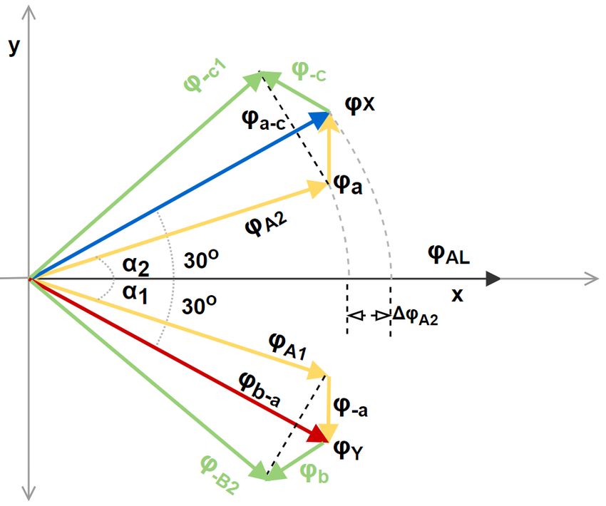
From the above equations it can be inferred that with inclusion of the bypasses the
flux through the two core rings A1 and A2 decreases which results in a reduction of
the projection of the two vectors on main flux. This reduction of projection results
in a decrease of loss angle α. This vector representation is illustrated further in the
Fig.3.4 illustrates the flux distribution in core after introducing bypass. The figure
illustrates the flux vectors and loss angle α for phase A. The remaining vectors are
symmetrical to phase A, but only 120◦ apart. Fig. 3.4.
Figure 3.4: Vector representation of flux with introduction of bypass
3.2 Types of Bypass configuration for Evans Core
There were several bypass configuration which can help reduce power losses in dis-
tribution transformers at no-load. But in this thesis, only three configurations were
used and their effect on loss reduction was analyzed. All the bypass configurations
part used were of Grain Oriented Steel and similar thickness as of the transformer
core individual sheets itself. There is not any specific name for the configuration,
so configurations are named according to type and a numeric suffix for the ease to
differentiate between them.
To construct the bypass configuration, two pieces each of bypass piece 1 or 2 de-
pending upon the bypass configuration were inserted between two layers of lower
143. Bypass
core ring and two layers from the outer core ring correspondingly. Two pieces of
bypass were inserted between the two slits. The idea behind this double layer by-
pass configuration is that it is faster to install. The illustration of how flux changes
direction is given in Fig. 3.5.
Figure 3.5: Orientation of flux in core and bypass
In Fig. 3.5, two bypass pieces were placed between the two successive core rings/sheets.
The arrow shows the direction of the flow of flux. By the introduction of bypass,
some amount of the flux flowing in the core rings, corresponding to the cross sectional
area of the bypass, starts flowing through the bypasses.
The Fig.3.6 is the first configuration of bypass and is named as configuration "EGO-
1". This bypass configuration was constructed with four different types of bypass
pieces for deflecting flux in the core rings. This bypass configuration consisted of
three sub-bypass configurations i.e., B1, B2 and B3. B1,the right most configuration
in Fig.3.6 for deflecting flux from lower core ring "C" to outer core ring "A" and the
B2 responsible for deflecting the flux from core ring "A" to the third core ring
"B". The B2 is responsible for bypassing flux between "B" and "C". Two five sided
polygon bypass pieces,on each side, between two successive core sheets and two
pieces between them deflects the flux from lower to upper or the other way around
in 4 steps each.
153. Bypass
Figure 3.6: Configuration of EGO-1
The Fig.3.7 is the second configuration of bypass and is named as configuration
"EGO-2". This bypass has the similar architecture as of the EGO-1 but the width
of bypass pieces is changed. In this configuration, the width of new bypass piece
was increased by 50% as of that used in previous configuration. The bypass piece
was wider in order to increase the cross section are of the bypass.
Figure 3.7: Configuration of EGO-2
The third type of bypass configuration used was different from the previously de-
scribed configurations. This configuration was named as "EGO-3" in which the flux
from the outer ring was shifted to a common piece connecting both the inner rings.In
Fig.3.8 this common piece is named N4. Same bypass piece as of the EGO-2 con-
figuration, was used in this configuration. Further a U-shaped piece with triangular
163. Bypass
faces on both sides was used to make a path for flux to flow from outer yoke to
the inner yokes. This configuration uses lesser material and has lower bypass to
core ration as compared to the other two configurations. The comparison of these
three configurations as per different parameters and their effect on loss reduction
are discussed in later chapter. The EGO-3 configuration is shown in Fig.3.8.
Figure 3.8: Configuration of EGO-3
173. Bypass 18
4
                          Methodology

In this chapter, the approach taken to carry out project is presented. This thesis
work is carried out in a structured approach. Further a brief description of each
stage is provided in the following sections.

4.1     Literature Review
The thesis started with intensive literature review. Since this thesis was based on
an innovative idea of development of a prototype therefore searching for the relevant
literature was challenging. However since work was previously done on such type
of a core, this provided a good starting point. Further different research papers
and journals were consulted for general behaviour of magnetic circuit and relevant
deductions were made about the shape of flux under the power electronics circuitry.

4.2     Experimental Setup
To evaluate the response of the magnetic core following properties were important
to examine:
   • Flux in the core leg.
   • Input power to no-load transformer
   • Flux in the bypass.
Flux in the main winding is crucial to examine the magnetic circuit of the trans-
former and inter-dependence and orientation of the flux inside the core.
Where as, since the transformer is operating on no load condition therefore the input
power constitutes the excitation losses.
For this a setup for measurement of these quantities was devised which is further
described in the next chapter.

4.3     Reference measurement
To begin with the reference measurement for the core was taken and verified against
the values obtained through previous studies. This was done to ensure the core still
retains its magnetic properties. This was also done to verify the measurement setup
used for the measurement of losses.

                                                                                  19
4. Methodology
Figure 4.1: Master thesis timeline
4.4 Power Electronic Circuit Development
Power electronics development was started with intensive literature studies. Once
the required configuration for the converter was determined, various components to
be used in such a converter were studied. Depending on the mode of operation a
complimentary configuration of converter was developed.
4.5 Evans Core measurement
Evans core as described in previous chapter like the Hexa-core is a wound core.
Therefore the behaviour of two cores is some what similar. However to establish a
reference working initially the Evans core was energized without any bypasses and
a reference loss curve was established. This reference loss curve provided excitation
losses against a range of operating flux in the main core. Later different types of
bypass arrangements were installed in the transformer and the results were compared
to previously established reference curve.
4.6 Data Acquisition & Analysis
After performing the practical measurement on the designed system, results were
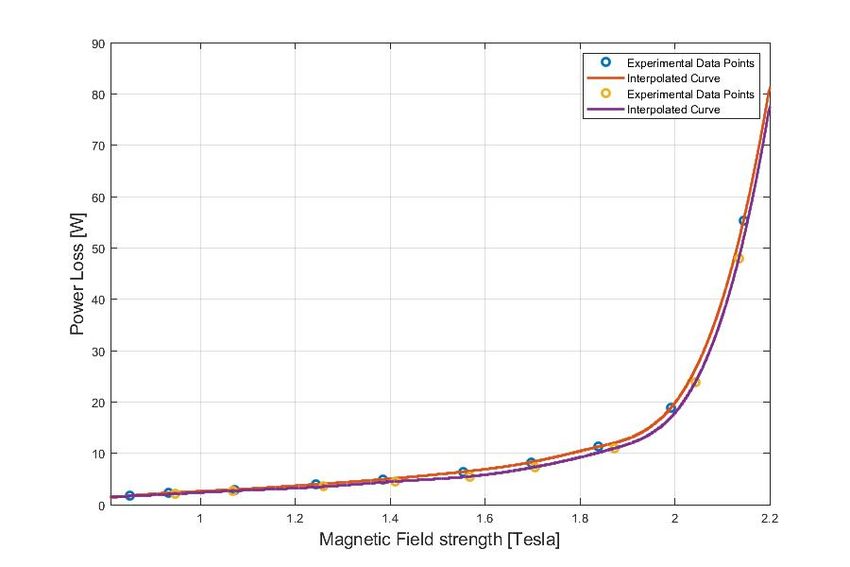
obtained. The obtained results are presented in the coming chapters. The results
are one dimensional interpolated to have a smoother curve, which in return helps in
predicting the behaviour of core through various data sets.
205
Measurement setup
For the analysis of both transformers, a measurement setup was developed. This
chapter focuses on the different measurement techniques used for measuring flux in
the core. Furthermore a so called active core control setup was developed to excite
the bypasses in order to reduce losses in the main core. Different measurement
equipment used during thesis are also discussed later in this chapter.
5.1 Transformer core
Transformer core used in this thesis was a down-scaled prototype of Evans core.
The core was made of M4-Oriented Carlite steel sheets of 0.27 mm thickness of
steel. The outer core was made by stacking 24 such steel sheets and the inner two
cores consisted of 23 steel sheets each. The transformer core was constructed with 1.0
mm wide slits (airgaps) between each two pair of steel sheets in the yoke in order to
able to adjust bypass pieces into the yokes. The physical specification of transformer
core and material specifications, provided by the manufacturer, are given in Tab. 5.1
Physical Specifications of Evans core
Specifications Unit Quantity
Width of steel sheet mm 40
Thickness of steel sheet mm 0.27
Volume of the core dm3 23.43
3
Density of Iron Kg/m 6.37
Weight of the core Kg 8.41
Number of outer sheets - 24
Number of inner sheets - 23
Stacking factor - 0.97
2
Cross-sectional area of leg mm 492.37
Table 5.1: Physical specification of Evans core
5.2 Core windings
There were two criterion for choosing the core windings. First criteria was the peak
currents through the winding during the region of high saturation. Magneto motive
215. Measurement setup
force mmf is the quantity, analogous to voltage in electric circuits, which gives rise
to magnetic fields. It depends upon the mean path length L and number of turns of
the coil N , magnetic flux Φ, the magnetic resistance to the field called as reluctance
< and the current through the coil I. By equating magneto motive force F for
magnetic intensity H and current in N turns of the coil, the high peak current in
the winding can be calculated as:
HL
I= (5.1)
N
It is a common practice to test distribution transformers at magnetic induction of
1.7 T or more. So in this thesis, measurements were being taken at 2.2 T as well, so
the maximum peak current was estimated according to 2.0 T . By using equation 5.1,
the peak current in the winding was found to be 11.82 A, so in order to withstand
such high current, a copper wire of diameter 3.5 mm was selected which has very
low resistance of 0.016 Ω per winding comprising of 120 turn each. Mean length of
each winding was 24 meters. Such low resistance contributes to less than 1% copper
losses in the winding even at the hard saturation region where magnetic induction
intensity is higher than 2.2 T , copper losses were less than 3.04 %. The selected
wire can also withstand high currents up to 50 A. Second criteria was to decide the
number of turns for each winding which in results dictates the magnetic flux flowing
through them. For such high voltages and magnetic induction, the number of turns
were decided to be 120 turns in total, three layers of 40 turns each were wound on
each leg.
5.3 RC integrator
To measure the flux magnitude in the core leg and bypasses, a so called low pass
filter was designed. This low pass filter is an RC integrator circuit with a feeding
voltage from the search coil. It attenuates the higher frequencies which are usually
in form of noise, and allows the low frequencies to pass.
Ideally such a filter, should have the components in such a way that:
1
ω >> (5.2)
RC
where as ω = 2πf . In principle at higher frequencies the capacitive reactance Xc is
quite low, where as it is very high as compared to the resistance at lower frequencies.
Having a lower capacitive reactance results in a negligible voltage drop on capacitor.
Since voltage across capacitor is proportional to the flux in the search coil, therefore
it gives a decent idea of shape and strength of magnetic flux inside the search coil.
The values for components in circuit implemented were chosen to be 470 nF and
100 Ω. Since it is a low pass filter so it tends to add a phase shift in the output
circuit which in case of implemented circuit was calculated to be 1.67◦ . The value
for phase shift is quite small there for it can be neglected in this application.
225. Measurement setup
Figure 5.1: An RC integrator circuit for flux measurement
5.4 Search coil magnetometer
A search coil is a wire wounded around a magnetic material to measure the change
in flux. It works according to Faraday’s law of induction. The changing magnetic
flux through the turns of the coil induces the voltage in the coil. This voltage is
given by:
dΦ
e = −N (5.3)
dt
where N is the number of turns and dΦ
dt
represents the changing magnetic flux in the
coil. The ” − ” sign represents opposite direction between both entities. A search
coil is illustrated in the Fig. 5.2
Figure 5.2: Search coil around magnetic flux carrying ferromagnetic material
In this thesis, the search coil of 10 turns was used for each measurement and ex-
citation of bypasses. In this thesis, search coils were used for measurement of flux
in both core types. Additionally these search coils were also used for the bypass
excitation in hexa-core. The number of search coils used for different measurements
in hexa-core and Evans core are given below:
1. List of different measurements for Hexa-core:
• one search coil each, for the excitation of six bypasses.
• one search coil each, for flux measurement in six bypasses.
• one search coil each, for flux measurement in all the three windings.
235. Measurement setup
2. List of different measurements for Evans core:
• one search coil each, for the measurement of flux in A1 and A2
• one search coil each, for flux measurement in bypass between A1 and A2.
5.5 Reference measurements for Evans and Hexa-
core
Reference measurements were taken for both transformer core types, hexa-core and
Evans-core. The reference measurement for the hexa-core transformer without by-
passes was extracted from the previous work on this transformer and is presented in
table below. In order to measure the loss reduction by introducing bypasses, a refer-
ence measurement or no-load measurement setup was developed. The transformer
was connected in delta configuration and was excited through a 3-phase auto trans-
former. A 3 phase digital power analyzer was used to measure the phase voltages,
phase currents and power losses in these windings. Transformer was connected to
the current transformer and potential transformer of the power analyzer in a 3 phase
3 wire configuration. This configuration is also known as two Watt-meter method
and is illustrated in the Fig. 5.3.
Figure 5.3: Two Watt-meter method
For the Evans core, a similar setup was established and is shown in Fig.5.4. In
this method, one Watt-meter measures the instantaneous power in phase A and the
other Watt-meter measures the instantaneous power in phase C and gives 3-phase
average power for the connected load.
Figure 5.4: Measurement setup for both transformers
245. Measurement setup
5.6 Bypass excitation
For bypass excitation a power electronics base active core strategy was developed
which is discussed in detail in the forthcoming chapter. The bypass was wound
with a coil and this coil was provided with a DC excitation source. The magnetic
field strength because of auxiliary flux in the bypass can be calculated using the
transformer formula: √
V = 2πf N ABmax (5.4)
Since the excitation coil is essentially an inductor wound around the bypass which
in this particular case behaves as the core for such inductor. When this inductor is
fed with a square wave from the converter, it behaves as a filter and the resultant
flux is a sinusoidal with a fundamental frequency of 50 Hz.
For this application, frequency is 50 Hz whereas area for bypass is given to be 30%
of the total cross section area of the core leg, number of turns for the auxiliary
windings on bypass was selected to be 10 turns. With these values the required DC
value for a particular magnetic field strength can be calculated.
255. Measurement setup 26
6
Flux Control Strategy
This chapter introduces the strategies utilized in controlling the flux in the trans-
former core. As described in previous chapters a strategy comprising of introducing
magnetic bypasses in the transformer can result in the reduction of excitation current
hence results in reduction of excitation losses. Since it was established previously
that Grain oriented bypasses have better performance as compared to Non-grain
oriented bypasses, therefore Grain oriented bypasses are used in this thesis.
6.1 Power Electronics Based Active Core
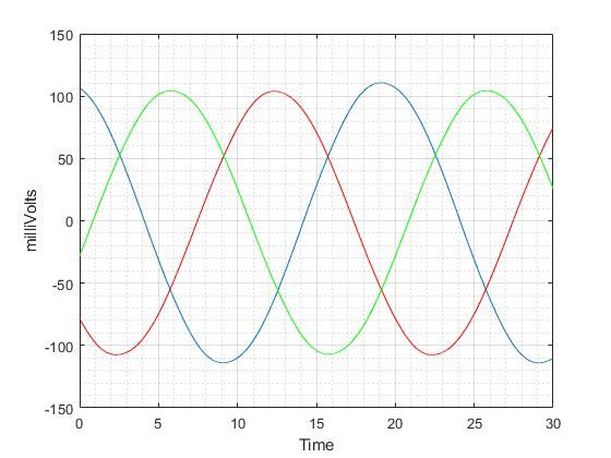
As shown in the Fig. 6.1 the shape of flux in the winding is sinusoidal and hence
it follows a hysteresis curve, where magnetic domains are aligned in both of the
cycles. So the aim was to assist in this change in domain alignment and as a result
excitation current from the supply can be reduced decreasing no-load losses.
Figure 6.1: Flux in 3-phases
To influence the shape of flux in the bypass a power supply based on the feedback of
main flux in the winding was designed. The main components of this power supply
are described in the following sections. Fig. 6.2 shows a schematic diagram of the
power electronics based power supply.
276. Flux Control Strategy
Figure 6.2: Schematics for active core flux control
6.1.1 Zero Crossing Detector
Since the bypasses are to be excited in synchronization with the point of zero cross-
ing of the flux therefore a feedback is required. This feedback can either be taken
from the flux in main winding or it can be taken from the flux in bypasses. But due
to physical as well as practical limits the feedback was not taken from the flux in
the bypasses.
An LM741 operational amplifier was implemented as a comparator so that a positive
pulse was triggered as the flux in the main winding crossed the zero crossing before
increasing to a positive value and zero pulse was triggered when the flux in the main
winding crossed zero before decreasing to a negative value. The input to this zero
crossing detector is taken from the output of search coil. The output waveform of
such a zero crossing detector is given in the Fig. 6.3.
Figure 6.3: Waveform for zero crossing detector
286. Flux Control Strategy
6.1.2 Controller
As previously discussed, flux in the main winding is chosen as reference for zero
crossing feedback, therefore a mathematical estimation for zero crossing in the by-
pass was implemented in a controller. From the previous work on the hexa-core
and bypasses, it is established that the phase difference between flux in the bypass
and main winding is 90◦ . Since the aim was to provide assistance during the period
where flux changes its direction, therefore the auxiliary excitation was provided 30◦
after the peak of flux in the bypass. Based on frequency of 50 Hz that translates
into 1.67 ms. So a delay of 1.67 ms was provided from the peak of the flux in the
bypass as shown in Fig, 6.4.
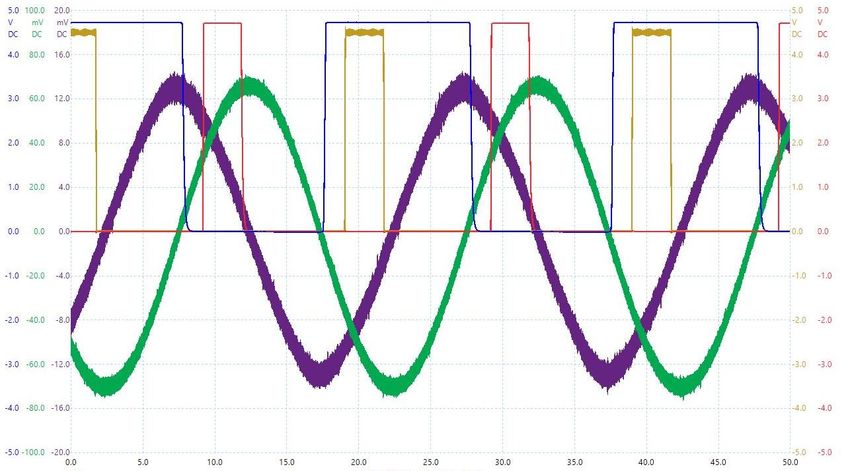
Fig. 6.4 illustrates the working waveform of this power electronics based active core
for one phase. The two sinusoidal waveforms represent the flux in main winding
(core-leg A) and the respective bypass a. Further a square pulse is triggered by
the controller at the zero crossing of the flux in main winding (green wave) and a
gate excitation pulse for Mosfet in H-bridge is triggered after a numerical delay to
synchronize with the bypass(purple wave).
In the waveform the position for excitation of one such bypass is given. Also one
thing to be noticed here is that since there are 6 bypasses so 6 such converters were
developed, one for each bypass. Since the bypass are constructed in a symmetrical
form therefore two such symmetrical bypasses on the either side of transformer will
have same zero crossing for flux but in opposite direction.
Figure 6.4: Excitation scheme for one bypass
Further to evaluate optimum point at which the bypasses could be excited the width
of this pulse was also set to variable which can be tuned in controller.
The outputs from the zero crossing detectors for 3 main windings provide input to
the controller and based on the calculations above outputs are provided to bridge
296. Flux Control Strategy
converter which can excite the bypasses through a DC source on during the time
calculated.
6.1.3 H-bridge Converter
A complimentary pair H-bridge converter was developed to excite the bypasses.
The IRF 2804 n-channel Mosfets and HA08p06 p-channel Mosfets were used. The
outputs of controller turn on and turn off Mosfets which in turn limits the operating
voltage range for the converter, but it simplifies the circuitry in comparison with
a dedicated gate drive circuitry. Fig. 6.5 shows the schematic for the H-bridge
topology for controlling flux in one bypass.
Figure 6.5: H-Bridge schematic for single bypass
The output of this converter is fed into a ten turn coil wound around the bypass
producing magnetic field in the coil. The direction of this magnetic field is dependant
on the voltage and magnitude of magnetic field is determined by the number of turns
and magnitude of voltage. Given by the following equation:
√
V = 2πf N ABmax (6.1)
So for current setup magnetic field of 1T is achieved by a voltage supply of 6 volts.
This is also to be mentioned that this 1T field is superimposed on already existing
field in the bypass. Since the coil wound around the bypass has a very small re-
sistance therefore a current limiting resistance is also installed at the output of the
current to limit the current which results an addition loss of 0.17 W . Six H-bridge
circuits were used in in order to control the flux in all three limbs.
307
Results
In this chapter the results measured from various operating conditions of power
electronics core are presented. Further the performance of Evans core and impact
of magnetic bypasses on such a core is also evaluated.
This is to be noted that a transformer is usually operated between magnetic field
strength which is lower then the saturation point which is around 1.9 T . Therefore
an operating range of 1.2 T to 2.0 T is selected to evaluate the response of the
developed prototypes.
In results the effect on two important quantities is evaluated. Firstly the no-load
power loss, which are basically the excitation losses and secondly the loss angle al-
pha. The loss angle, alpha is the angle between A2 and the leg as described in the
previous chapters. The usual value for this loss angle with grain oriented bypass was
previously established to be 27◦ in case of hexa-core. Therefore figures illustrating
comparison between previously established loss angle and impact of bypass excita-
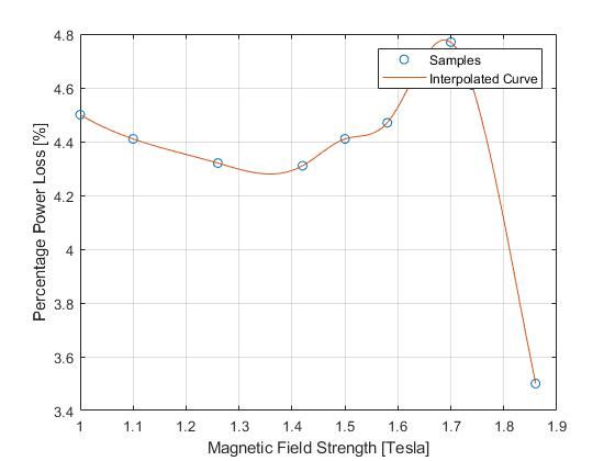
tion are presented in this chapter.
The value for loss angle in case of an Evans Core is also determined graphically
which is presented in the later sections. The emphasis on role of this loss angle in
performance of transformer is described in previous chapters.
7.1 Loss reduction with Active Core
In this section the influence of active core on the excitation losses in transformer is
presented. A step by step approach was taken in order to evaluate the outcomes,
and the outcomes are presented in the following sections.
7.1.1 Influence of each bypass
Since it is very important to know, how much flux in the transformer can be in-
fluenced with excitation of each bypass. Therefore bypass excitation was added
progressively and the change in loss angle and excitation loss was recorded. The
operating value of excitation level was selected to be 1.5 T in the main core which
gives an operating voltage of 18.5 V . The input DC excitation voltage was at 6 V
so that the auxiliary exciting level in the bypass is around 1 T . Tab. 7.1 shows the
31You can also read