The Effect of Seasonal Climatic Anomalies on Zoo Visitation in Toronto (Canada) and the Implications for Projected Climate Change - MDPI
←
→
Page content transcription
If your browser does not render page correctly, please read the page content below

atmosphere
Article
The Effect of Seasonal Climatic Anomalies on Zoo
Visitation in Toronto (Canada) and the Implications
for Projected Climate Change
Micah J. Hewer 1, * and William A. Gough 2
 1   Department of Geography, University of Toronto, Toronto, ON M5S 3G3, Canada
 2   Department of Physical and Environmental Sciences, University of Toronto Scarborough, Toronto,
     ON M1C 1A4, Canada; gough@utsc.utoronto.ca
 *   Correspondence: micah.hewer@mail.utoronto.ca; Tel.: +1-289-880-8502

 Academic Editors: Daniel Scott and Stefan Gössling
 Received: 15 April 2016; Accepted: 18 May 2016; Published: 23 May 2016

 Abstract: This study uses a multi-year temporal climate analogue approach to explore zoo visitor
 responses to seasonal climatic anomalies and assess the impacts of projected climate change on
 zoo visitation in Toronto, Canada. A new method for selecting a representative weather station
 was introduced which ranks surrounding stations based on “climatic distance” rather than physical
 distance alone. Two years representing anomalously warm temperature conditions and two years
 representing climatically normal temperature conditions were identified for each season from within
 the study period from 1999 to 2015. Two years representing anomalously wet precipitation conditions
 and two years representing anomalously dry precipitation conditions were also identified. F-tests
 and t-tests were employed to determine if the apparent differences in zoo visitation between the
 temperature and precipitation paired groupings were statistically significant. A “selective ensemble”
 of seasonal Global Climate Model (GCM) output from the Intergovernmental Panel on Climate
 Change Fifth Assessment Report was used to determine when these anomalous temperature and
 precipitation conditions may become the norm in the future. When anomalously warm winters
 and springs occurred within the historical record, total zoo visitation in those seasons increased
 significantly. Inversely, when anomalously warm summers occurred, total summer season zoo
 visitation decreased significantly. Temperature anomalies in the autumn season did not result in
 any significant differences in total autumn season zoo visitation. Finally, apart from in the spring
 season, there were no significant differences in total zoo visitation between anomalously wet and
 dry seasons.

 Keywords: tourism climatology; seasonal climatic anomalies; temporal climate analogue; climate
 change impacts; outdoor recreation and tourism; zoo visitation

1. Introduction
     For decades, it has been acknowledged [1–3], and is now generally accepted [4,5], that weather
and climate affect behaviour and satisfaction associated with outdoor recreation and tourism.
Nonetheless, the relationship between weather with recreation and tourism is poorly understood and
under-researched [6–8]. More specifically, very little is known about the specific weather sensitivity of
particular tourism attractions within urban areas [9–12].
     Zoological parks serve as excellent case studies in the field of tourism climatology because zoos
can provide accurate records of visitor attendance data over time since they must account for all
visitors on their property for financial and liability reasons [13]. Recently, there has been a number of
studies aimed at assessing the weather sensitivity of zoo visitation [9,11–13]. However, no study to

Atmosphere 2016, 7, 71; doi:10.3390/atmos7050071                          www.mdpi.com/journal/atmosphere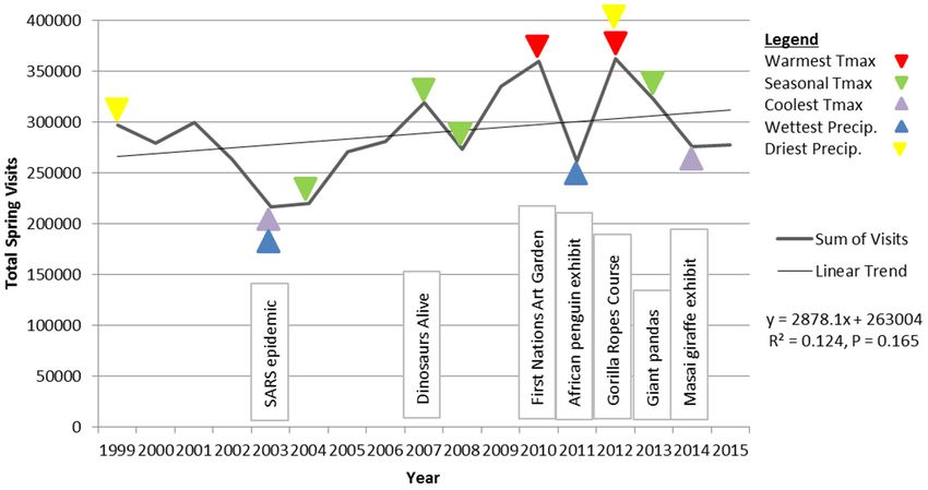
Atmosphere 2016, 7, 71                                                                               2 of 20

date has looked at the effect of seasonal climatic anomalies on zoo visitation, nor tried to understand
the implications of climate change for zoo visitation using a temporal climate analogue approach.
     Dwyer [14] suggested that if daily temperatures exceed seasonal averages during cold weather
months, recreation participation is likely to increase, whereas during warm weather months, if daily
temperatures exceed the seasonal average, participation may decline. In theory, warm, dry days should
encourage visits; whereas, hotter weather may drive potential visitors to alternative attractions, such
as indoor venues or participation in water-related activities [15]. This study aims to test these previous
conclusions regarding demand responses to seasonal climatic anomalies for outdoor recreation and
tourism (ORT), this time in the context of an urban zoological park.
     Being pioneered by Glantz [16–18], analogues can be spatial in nature, where insights are drawn
from a comparable region or location to the case study; or temporal, where analysis of past conditions
is used to develop an understanding. Both spatial and temporal analogues aim to help assess impacts
while identifying and characterizing determinants, using what is known about the present to make
inferences about the future [19]. The use of analogue methodologies overtime has significantly
increased current understanding of how climate affects society, including impacts, vulnerability, and
adaptive capacity [19]. Historical analysis through the use of temporal analogues allows for the
characterization of how human systems manage and experience climatic risks [20]. According to
Ford et al. [21], the temporal analogue approach is based on the premise that human systems in the
near future will probably conduct activities as they have done in the recent past and be influenced
by similar conditions and processes, providing empirical grounding to the analysis of sensitivity,
vulnerability, and adaptation in climate change impact assessment.
     The analogue approach has been severely under-utilized in climate change and tourism
studies [22–25], although it has the potential to offer new insights into future impacts and the
effectiveness of adaptations [23]. Analogues are a useful tool for identifying the possible future
impacts of global climate change, as impacts are assessed during real events and include adaptation
strategies and business decisions made during an anomalous “short term” event, which may become
the norm in the future [24]. A key advantage of the climate change analogue approach is that it
captures the full range of supply-side and demand-side adaptations by tourism operators, destination
marketers, and tourists themselves [26]. This study aims to use a temporal analogue approach to
determine if any further insights into the implications of climate change for zoo visitation can be gained,
with particular relevancy to the recent modeling approach for assessing the impact of climate change
on zoo visitation [27]. Analogues have been promoted as a simple and effective validation tool for
more sophisticated modeling approaches [26], such as the recent works by Hewer and Gough [12,26].
The analogue approach is also less subject to the high levels of uncertainty associated with complex long
range models. Furthermore, analogues provide insights into fully contextualized actual adaptation,
while regression analysis can only offer highly abstracted projections of potential adaptation (personal
communication on 13 May 2016: Professor Daniel Scott, University of Waterloo).
     In the context of ski tourism [24,25], the temporal climate analogue approach has revealed more
conservative assessments of the impact of projected climate change on ski season length and lift ticket
sales, when compared to the physical modelling approach [28,29]. Furthermore, Scott [23] found that
the decline in skier demand using a climate analogue approach was far less than survey studies of
hypothetical behaviour change had projected [30,31]. When reviewing tourism demand response
studies in the field of tourism climatology, Gössling et al. [32] concluded that econometric modelling
studies have a wide range of uncertainties with regard to behavioural response, but climate analogues
may provide more robust insights. Scott et al. [28] suggested that tourists have the greatest capacity
to adapt to the risks and opportunities posed by climate change, a factor responsible for much of the
uncertainty in the modelling approach. However, Scott et al. [26] contend that there remains much
scope to better understand the adaptive capacity of tourists and tourism operators alike, by assessing
climate analogue events.
     Aylen et al. [9] were the first to analyse historical weather and attendance data in an effort to
explore the weather sensitivity of zoo visitation. Based on a case study of Chester Zoo in the United
Kingdom, the authors concluded that visitor behaviour was mainly influenced by the annual rhythm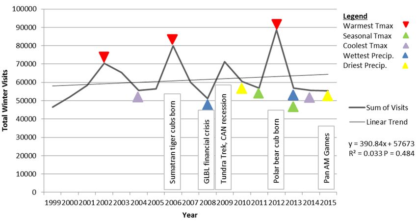
Atmosphere 2016, 7, 71                                                                                 3 of 20

of the year and the pattern of school and bank holidays. However, there was evidence that visits were
redistributed over short periods of time in accordance with the weather [9]. The results suggested
that visitors who may have been frustrated by rainy weather one day; turn up later when the weather
improves [9]. Furthermore, the authors suggested that although warmer temperatures encourage
visits, this relationship was only maintained up to a threshold level of approximately 21 ˝ C. Finally,
this preliminary study found no evidence of a long-run shift in behaviour due to climate trends; but
rather, just an immediate response to each day’s weather [9]. In conclusion, Aylen et al. [9] essentially
dismissed any considerable seasonal or annual impacts of projected climate change on zoo visitation.
       Perkins [13] tested the applicability of the spatial synoptic classification (SSC) as a tool to predict
visitor attendance response in the tourism, recreation, and leisure (TRL) sector across different climate
regimes, based on a case study using 10 years of daily attendance data from two different zoological
parks in Atlanta and Indianapolis, USA. Daily attendance data was paired with the prevailing synoptic
weather conditions to assess the potential impacts that ambient atmospheric conditions had on visitor
attendance [13]. The results indicated that dry moderate conditions were most associated with high
levels of attendance and “moist polar” synoptic conditions were most associated with low levels of
attendance at both zoological parks [13]. However, the author concluded that visitors in Indianapolis
showed lower levels of tolerance to synoptic conditions which were not “ideal”; being more averse
to “polar” synoptic regimes and less tolerant to “moist tropical” synoptic regimes. Although optimal
conditions for zoo visitation may be generalizable across different geographic locations with varying
climatic conditions; visitor perception of, and response to, unfavourable weather conditions seem to
vary between different case studies.
       Perkins and Debbage [11] focused on ambient thermal environments and visitor behaviour at
zoological parks in Phoenix and Atlanta, USA. The authors analysed 10 years of daily zoo visitation in
concert with daily weather data to establish the Physiologically Equivalent Temperature (PET) and
measure the thermal conditions most likely experienced by zoo visitors. The results suggested that
although optimal thermal conditions associated with both zoos appeared to be the same (“slightly
warm” or “warm”, based on PET thermal categories); thermal aversion occurred on opposite sides of
the spectrum, with visitors in Atlanta avoiding extreme cold and those in Phoenix adverse to extreme
heat [11]. This study has important geographic implications for the weather sensitivity and thermal
thresholds associated with zoo visitation; nonetheless, the authors called for further research focusing
on zoological parks in cooler climates than that which is characteristic of Atlanta.
       Hewer and Gough [12] used 15 years of daily weather and attendance data to create predictive
regression models in an effort to determine the seasonal weather sensitivity of visitation to a zoological
park in Toronto, Canada. The results suggested that shoulder season months (spring and fall)
were most weather sensitive, followed by off-season months (winter) and then peak-season months
(summer). Furthermore, the authors also identified weather-related behavioural thresholds for zoo
visitation. During the shoulder season, temperatures exceeding 26 ˝ C were indicative of a critical
temperature threshold, causing attendance levels to decline. In the peak season, visitors were more
tolerable of extreme heat and attendance levels did not decline until temperatures exceeded 29 ˝ C [12].
For precipitation, average daily attendance levels declined by approximately 50% when only trace
amounts of precipitation was recorded on a given day (0.2 to 2.0 mm). Interestingly, there was very
little additional decline in attendance as the volume of total daily precipitation increased beyond 2 mm,
including days that recorded more than 60 mm of total precipitation [12]. The authors concluded that
maximum temperature was the most influential weather variable during the off and shoulder seasons;
however, total precipitation was the most influential weather variable in the peak season.
       The first formal climate change impact assessment on zoo visitation was conducted by Hewer and
Gough [27], using a modelling approach to predict seasonal and annual impacts of projected climate
change, based on regression equations derived from the statistical relationship between daily weather
and zoo attendance. In regard to annual impacts, the modelling results suggested that visitation is
likely to increase by 8% as early as the 2020s (2011 to 2040), by 14%–17% in the 2050s (2041–2070), and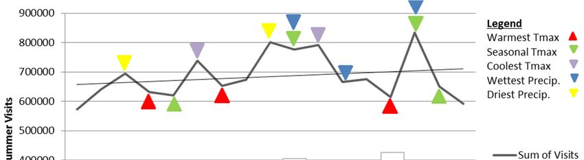
Atmosphere 2016, 7, 71 4 of 20
by 18%–34% in the 2080s (2071–2100); the range of impacts are dependent upon low and high emissions
scenarios and their associated degrees of warming. In regard to the impacts on seasonality, the authors
Atmosphere 2016, 7, 71 4 of 20
concluded that the off-season would experience minor increases in attendance, while the majority of
increases would
and high be experienced
emissions during
scenarios and their the shoulder
associated seasons.
degrees However,
of warming. increased
In regard to thewarming
impacts on under
projected climate change was predicted to have a negative effect on peak season
seasonality, the authors concluded that the off-season would experience minor increases in visitation, especially if
warming exceedswhile
attendance, ˝
3 C the
during the summer
majority months
of increases [27].
would beThe current study
experienced duringaims
the to compare
shoulder the results
seasons.
of theHowever,
modelling increased
approachwarming
and theunder projected
analogue climate to
approach change was predicted
assessing the impact to of
have a negative
projected climate
effect on peak season visitation,
change on zoo visitation in Toronto. especially if warming exceeds 3 °C during the summer months [27].
The current study aims to compare the results of the modelling approach and the analogue approach
to assessing the impact of projected climate change on zoo visitation in Toronto.
2. Methods
2. Methods
2.1. Data
The Toronto Zoo (Figure 1) supplied quantitative data describing the total number of daily zoo
2.1. Data
visitors from January 1999 to December 2015. Unfortunately, the supplied data did not distinguish
The Toronto Zoo (Figure 1) supplied quantitative data describing the total number of daily zoo
between different
visitors types 1999
from January of visitors (individuals,
to December couples, families,
2015. Unfortunately, organized
the supplied data didgroups, season pass
not distinguish
holders); nor did the data set provide any qualifying information such as distance
between different types of visitors (individuals, couples, families, organized groups, season pass travelled to reach
the zoo (local nor
holders); residents,
did thedomestic tourists,
data set provide anyinternational tourists) orsuch
qualifying information anyasdemographic information
distance travelled to reach such
as agethe
orzoo
gender. Furthermore,
(local residents, the data
domestic set international
tourists, did not indicate theor
tourists) timing of visitationinformation
any demographic on a particular
such day
as agemeasured
(not being or gender. Furthermore,
on an hourlythe data
time set did
scale). not indicate
Finally, the timingrecord
the visitation of visitation on a particular
associated day
with a zoological
(not being measured on an hourly time scale). Finally, the visitation record associated with
park is certainly dynamic in nature, as it is frequently affected by internal and external factors such as a zoological
park isof
the arrival certainly dynamic
new animal in nature, the
attractions, as itopening
is frequently affected
of new zoo by internalasand
exhibits external
well factors such
as prevailing as and
social
the arrival of new animal attractions, the opening of new zoo exhibits as well as prevailing social and
economic conditions. More detailed discussion of the way these factors affect the zoo visitation record
economic conditions. More detailed discussion of the way these factors affect the zoo visitation record
by introducing new dynamics into the time series data, as well as how they were controlled for within
by introducing new dynamics into the time series data, as well as how they were controlled for within
this study, emerge
this study, throughout
emerge throughoutthis paper.
this paper.Nonetheless,
Nonetheless, 17 17 years
yearsofofdaily
daily
zoozoo visitation
visitation datadata provided
provided a a
rich historical record
rich historical from
record which
from whichtotoconduct
conductaameaningful analysisconcerning
meaningful analysis concerning thethe impact
impact of seasonal
of seasonal
climatic anomalies
climatic anomalieson on
zoozoo
visitation
visitationin
inToronto, Ontario(Canada).
Toronto, Ontario (Canada).
Buttonvillle A
Metro Zoo
Lake Ontario
Pearson Int’l A
CANADA
USA
Figure 1. Map of the Toronto area showing location of the Toronto Zoo (formerly the Metro Zoo) and
Figure 1. Map of the Toronto area showing location of the Toronto Zoo (formerly the Metro Zoo) and
nearby weather stations.
nearby weather stations.
Typically, for studies in tourism climatology and climate change impact assessments for
Typically, for studies
tourism, weather inobtained
data is tourismfrom
climatology
the closestand climate change
meteorological impact
station assessments
in proximity for tourism,
to the tourism
weather data [12,27,33,34].
attraction is obtainedHowever,
from theprevious
closesttourism
meteorological
climatologystation
studies in
andproximity to the
climate change tourism
impact
assessments
attraction for tourism
[12,27,33,34]. have been
However, criticised
previous for using
tourism climate datastudies
climatology from weather stationschange
and climate which are
impact
located a considerable distance from the attraction itself, due to the presence
assessments for tourism have been criticised for using climate data from weather stations which of microclimates
Atmosphere 2016, 7, 71                                                                                                5 of 20

are located a considerable distance from the attraction itself, due to the presence of microclimates
associated with many tourism destinations [35,36]. The current study was positioned to introduce a
new method for selecting the most representative weather station since there was daily meteorological
data recorded by a former Environment Canada weather station at the study site itself, for the period
from January 1977 to December 1992. Based on the map coordinates for the Metro Zoo station (43˝ 491 N,
79˝ 111 W) provided by Environment Canada, this station was situated in the south east area of the
current Toronto Zoo property. The current study required daily weather data from 1981 to 2010 to
establish the baseline climate conditions for the region, as well as daily weather data from 1999 to
2015 to assess the impact of seasonal climatic anomalies on zoo visitation. Rather than selecting a
weather station based on physical distance alone, this study ranked the five closest weather stations in
proximity to the Toronto Zoo (Figure 1), based on their ability to represent average monthly climate
conditions recorded at the Metro Zoo station from 1977 to 1992. Daily weather data was available for
each of the test stations from 1977 to 1992, except for the Buttonville A weather station, which only
had data from 1987 to 1992.
     In order to establish the climatic distance (Cdist) for each weather variable (Wi ) considered
(maximum temperature and total precipitation) the average monthly value for the test station was
subtracted from the average value measured at the zoo (Wz ) and then the difference was squared. Once
this had been completed for each month from 1977 to 1992, the mean value was then taken, Σ, and
divided by the standard deviation squared, δ2 , of the average monthly values for the selected weather
variable that was measured at the zoo. Finally, the square root of this resulting value was calculated to
determine the Cdist (1) between each test station and the zoo for both maximum temperature (Tmax)
and total precipitation (Ptot).
                                   Cdist “ pΣppWi ´ Wz q2 q{δz 2 q1/2                                 (1)

      In theory, if all the weather measurements recorded at the zoo were identical to those recorded at
a particular test station, the resulting value derived from the Cdist formula would be zero. Therefore,
stations that recorded resulting values for Cdist closest to zero were determined to have weather
conditions most similar to those recorded at the zoo station. The Cdist value was then used to rank the
different weather stations for both climatic variables of interest in this study (Table 1). Next, the mean
rank for each station was determined by averaging the numerical rank each station received in relation
to both Cdist values. It is interesting to note that the weather station which recorded average monthly
Tmax and average monthly Ptot values most similar to those recorded at the zoo itself was the station
located farthest from the zoo in relation to the other four test stations. The Toronto Lester B. Pearson
International Airport (Pearson A) weather station recorded the closest Cdist for Tmax and the second
closest Cdist for Ptot, resulting is the lowest mean rank (1.5). Although the Pearson A weather station
was farthest from the zoo in regard to physical distance (37.8 km), it was the station that shared the
most similar elevation with the zoo (being situated only 30.1 m higher); whereas, the closest weather
station (Buttonville A, 15.3 km away), was situated 54.8 m higher than the zoo station. Apart from
physical distance and elevation, other environmental features which are characteristic of the climate in
this region, such as the urban heat island and lake breeze effects [37,38], likely influenced the ability of
these different weather stations to represent the atmospheric conditions recorded at the zoo.

     Table 1. Climatic Distance (D) for the Toronto Zoo (based on an analysis of observational data from
     1977 to 1992).

     Weather Station      Physical D (km)     Elevation D (m)      Tmax D (Rank)       Ptot D (Rank)      Mean Rank
      Buttonville A             15.3                +54.8             0.0852 (5)         0.0645 (1)            3
      Richmond Hill             21.5                +96.7             0.0728 (3)         0.0711 (5)            4
         Toronto                23.6                ´30.8             0.0683 (2)         0.0693 (4)            3
         Oshawa                 27.6                ´59.5             0.0829 (4)         0.0692 (3)           3.5
        Pearson A               37.8                +30.1             0.0681 (1)         0.0687 (2)           1.5
        Note: Distance for all variables established based on a comparison with observational data (1977–1992) from
        the weather station at the former Metro Zoo (Location: 43˝ 82’N, 79˝ 18’W; Elevation: 143.3 m).
Atmosphere 2016, 7, 71 6 of 20
In order to employ a temporal climate analogue approach [23–25] for assessing the impact of
climate change on participation in tourism and recreation, it is necessary to refer to the available
projections for future climate in this region. Global Climate Model (GCM) output from the
Intergovernmental Panel on Climate Change (IPCC) 2013 Fifth Assessment Report (AR5) can be
obtained from the Coupled Model Inter-comparison Project of the World Climate Research Programme.
However, there is a wide selection of GCMs available to provide projections of future climate change,
40 in total from the most recent assessment. Furthermore, each of the 40 modelling centres provide
future projections for the four different Representative Concentration Pathways (RCPs), which describe
how Green House Gas (GHG) concentrations could evolve over the next 100 years and thereby influence
global climate. There are many approaches that have been developed in order to provide some direction
for determining which of the future projections of climate available for impact assessments should
be used in planning [39]. Compared against historical observed gridded data, climate projections
using the ensemble approach have been shown to come closest to replicating the historical climate [40].
This approach suggests that it is best to plan for the average climate change from all the climate model
projections by using a mean of all the models to reduce the uncertainty associated with any individual
model [27]. In effect, the individual model biases seem to offset one another when considered together.
It is generally accepted that climate models can be evaluated based on their ability to reproduce
baseline conditions [41]. However, some climate models perform better in certain regions than they do
in others. For this reason, it is unreasonable to create a “full” ensemble including all of the available
GCMs when it is evident that some models are unable to reproduce past climate for the study region.
Based on this logic, it is more appropriate to evaluate each model individually, based on its ability to
reproduce past climate, and then rank and select the best three models to create a “selective” ensemble
from these top performing models [27]. Greater detail pertaining to the process of ranking and selecting
GCMs for climate change impact assessment, including the use of the Gough-Fenech Confidence Index
and the creation of selective ensembles is available elsewhere [27]. Table 2 presents a selective ensemble
of seasonal GCM output for Tmax and totP at Pearson A from 2011 to 2100 under RCP4.5 and RCP8.5.
As described by the IPCC [41], RCP4.5 represents a low radiative forcing, stabilization scenario; while
RCP8.5 represents a high radiative forcing, increased emissions scenario.
Table 2. Selective Ensemble of Seasonal GCM Output for Maximum Temperature and Total
Precipitation at Toronto Lester B. Pearson International Airport from 2011 to 2100 under RCP4.5
and RCP8.5 Climate Change Scenarios.
Season 2020s 2050s 2080s
Projected Change in Maximum Temperature (˝ C)
Winter 1.19 to 1.33 2.49 to 2.98 2.59 to 5.19
Spring 1.50 to 1.52 2.44 to 3.31 3.17 to 5.30
Summer 1.53 to 1.54 2.85 to 3.86 3.70 to 6.77
Autumn 1.63 to 1.64 2.54 to 3.39 3.10 to 5.70
Annual 1.30 to 1.34 2.69 to 3.23 3.19 to 5.13
Projected Change in Total Precipitation (%)
Winter 10.3 to 10.9 9.9 to 21.6 17.9 to 29.3
Spring 3.9 to 6.4 9.3 to 14.1 8.3 to 24.8
Summer 3.5 to ´4.3 ´6.7 to ´2.1 ´6.9 to ´9.8
Autumn ´4.7 to 0.3 ´1.9 to 3.5 ´0.6 to 1.0
Annual 3.7 to 3.8 8.0 to 9.0 6.9 to 13.6
2.2. Analysis
Seasonal climatic anomalies were identified by first determining the seasonal climate normals
(30 year averages), for both daily maximum temperature (Tmax) and daily total precipitation (totP)
at Pearson A weather station from 1981 to 2010. Once the climate normals were determined for eachAtmosphere 2016, 7, 71 7 of 20
season, it was then possible to identify which years (if any) recorded anomalously warm or wet winters,
springs, summers, and autumns. Previous climate change impact assessments for tourism [23–25]
which have applied similar methodological approaches (temporal climate analogues), relied on only
one season or year for their analysis. This limitation of previous research is subject to potential bias from
unidentified non-climatic factors that may have either increased or decreased tourism participation in
that same season/year, but the results were attributed to the anomalous climate conditions nonetheless.
Using the rich historical record of daily visitation data supplied by the Toronto Zoo, the current study
was able to identify two climatic anomalies for each season from which to base conclusions upon;
thereby reducing the potential effect that non-climatic factors occurring in a given year may have
had on the reported results. Therefore, for each season, the two years which recorded the warmest
temperatures (from 1999 to 2015), along with the two years that recorded temperature closest to the
seasonal average (relative to the 1981 to 2010 baseline), as well as the two years that recorded the
coolest temperatures were all identified. Furthermore, for each season, the two years which recorded
the greatest volume of total precipitation (the two wettest seasons), along with the two years that
recorded the lowest volume of total precipitation (the two driest seasons), were also identified.
The analysis was conducted individually for each season and the same methods were repeated
therein. To begin, daily zoo visitation data was aggregated to seasonal averages to assess the impact
of seasonal climatic anomalies using the standard climatic interpretation of seasons in the region:
Winter (December, January, February); Spring (March, April, May); Summer (June, July, August);
and Autumn (September, October, November). The total number of annual zoo visitors within a
particular season was then graphed over time. In order to explore the stationarity of total seasonal
zoo visitation over time, the equation for the slope of the linear trend line was determined and a
simple linear regression analysis was conducted. This determined whether total seasonal visitation
had been increasing/decreasing over time, and whether the observed trend was statistically significant;
which guided the selection of climate analogues and climate normals. If there was not a statistically
significant trend associated with total annual zoo visitation in a given season, then there was no need
to defer from selecting a climatically anomalous or normal year that occurred near the beginning
or end of the data set. However, if the linear trend was found to be statistically significant then it
would be beneficial to avoid years near the beginning or end of the data set since they may have been
negatively or positively influenced by the slope of the linear trend line. The identified seasonal climatic
anomalies and climate normals were then specified on each graph to create a visual demonstration of
the effect these seasonal occurrences may have had on total visitation that year.
In order to assist in the interpretation of results associated with the impact of seasonal climatic
anomalies on zoo visitation in Toronto, qualitative information on important non-climatic variables
was obtained from the zoo’s official website [42]. Table 3 lists a number of important non-climatic
factors (internal factors appear in black while external factors are in red) for each year, covering the
entire temporal scope of the study (1999 to 2015). The most notable of these non-climatic factors were:
the negative impact of SARS in 2003; the positive impact of the new Dinosaurs Alive exhibit in 2007;
the positive impact of the two new Giant Pandas in 2013 and the negative impact from the competing
presence of the PAN-AM Games in 2015. This information helped to understand the over-riding effect
certain internal (special animal attractions, new exhibits) or external (disease, recession, competing
events) factors may have had on seasonal zoo visitation during a given year, regardless of the prevailing
climatic conditions. These non-climatic factors were then specified on the same graph that illustrated
the annual fluctuations in total zoo visitation, as well as the climatic anomalies and climate normals,
within a given season. This created a useful visual cross-reference to check what other factors may have
been involved in a particular year that seasonal visitation was either high or low due to a particular
climatic anomaly.
Once the effects of the climatic anomalies within a particular season were visually observed
within the graphs, a series of statistical tests were employed to determine if the observed differences
were statistically significant. For temperature, the daily data from the two years that represented theAtmosphere 2016, 7, 71 8 of 20
climatic anomalies were tested against the daily data from the two years that represented climate
normals to see if there were significant differences between the variances and means of the two groups
(using F-tests and t-tests, respectively). For precipitation, daily data from the two years representing
the wettest seasons was test against the two years representing the driest seasons; again, using F-tests
and t-tests to see if there were significant differences between the variances and means of the two
groups, respectively.
Finally, the impact of projected climate change on zoo visitation was assessed using a temporal
climate analogue approach. In this regard, the climatic anomalies recorded in each season were
cross-referenced against the climate change projections for the span of the 21st century in this region,
based on the selective ensemble of seasonal GCM outputs. It was then possible to provide predictions
concerning when these climatic anomalies may potentially become climate normals in the future,
under projected climate change. It has been suggested by Scott et al. [26] and Gössling et al. [32] that
this approach is a useful tool for climate change impact assessment since it captures both supply and
demand side adaptation to anomalous climatic conditions.
Table 3. Annual history of new zoo exhibits, special animal attractions, and major external factors from
1999 to 2015.
Year New Zoo Exhibits, Special Animal Attractions, External Factors
2015 First giant panda cubs born in Canada; Pan Am Games in Toronto
2014 First Burmese star tortoise hatches in Canada; Masai Giraffe Exhibit opens
2013 A pair of giant pandas arrive on loan for five years from China; polar bear cub is born
2012 Gorilla Ropes Course opens; three new white lions arrive
2011 African penguin exhibit opens; polar bear cub is born
2010 Conservation Carousel opens; First Nations Art Garden opens
Award-winning Tundra Trek exhibit opens; two snow leopard cubs are born;
2009
Western Lowland gorilla is born; Canadian economic recession
2008 Great Barrier Reef opens; Stingray Bay opens; Global financial crisis
2007 Two Amur (Siberian) tiger cubs born; Dinosaurs Alive opens
2006 Two Sumatran tiger cubs are born
2005 Male gorilla born
2004 Discovery Zone: Kids Zoo opens
Discovery Zone: Amphitheater opens; first birth of three Sumatran tigers in Canada;
2003
first hatchings of Komodo dragons in Canada; SARS crisis in Toronto
2002 Discovery Zone: Splash Island opens; two koalas on exhibit for the summer
2001 Award-winning Gorilla Rainforest exhibit opens
2000 Eyelash vipers go on display
1999 Indo-Malaya Fish Capital project completed introducing new freshwater exhibits
3. Results
In regard to the presence of confounding non-climatic factors, there were no special animal
attractions or new zoo exhibits which would have been likely to explain the unusually high number
of zoo visitors during the anomalously warm winters of 2006 and 2012. Furthermore, there were not
any known external factors which would have been likely to reduce total visitation during the winters
that recorded seasonal temperatures (2011, 2013). In regard to total precipitation, there did not seem
to be any internal confounding factors during the anomalously wet or dry winter seasons. However,
the wet winter of 2008 was concurrent with the global financial crisis which seems to have a positive
effect on zoo visitation that year and the dry winter of 2015 was concurrent with the Pan Am Games in
Toronto which seemed to have a negative effect on zoo visitation that year. Nonetheless, it unlikely
that the influence of these non-climatic factors which occurred in only one of the two years for both the
wet and dry anomalous year groupings skewed the results dramatically, especially since the Pan Am
Games was a summer event and may not have had much impact on winter season visitation that year.
In regard to the presence of confounding non-climatic factors, there were no special animal
attractions or new zoo exhibits which would have been likely to explain the unusually high number
of zoo visitors during the anomalously warm springs of 2010 and 2012. Furthermore, there were not
any known external factors which would have been likely to reduce total visitation during the springsAtmosphere 2016, 7, 71 9 of 20
Atmosphere 2016, 7, 71 9 of 20
that recorded seasonal temperatures (2004, 2008). In regard to total precipitation, the anomalously wet
springany known
season external
of 2003 wasfactors
also the which
secondwould have
coolest been recorded
spring likely to between
reduce total
1999visitation
and 2015. during the
Furthermore,
springs that recorded seasonal temperatures (2004, 2008). In regard to
this season was also concurrent with the SARS crisis in Toronto, which had a negative impact total precipitation, the on
anomalously wet spring season of 2003 was also the second coolest spring recorded between 1999
zoo visitation that year. These two confounding variables were likely to exaggerate the impact that
and 2015. Furthermore, this season was also concurrent with the SARS crisis in Toronto, which had a
the anomalously wet season had of total spring zoo visitation. However, it is unlikely that their
negative impact on zoo visitation that year. These two confounding variables were likely to
presence wouldthe
exaggerate negate
impactthe
thatresults altogether,wet
the anomalously especially
season had since thespring
of total anomalously wet spring
zoo visitation. However, of 2011
causedit is unlikely that their presence would negate the results altogether, especially since the the
similar effects when no other confounding factors appeared to be present. Furthermore,
anomalously
anomalouslydry wet
season of 2012
spring was
of 2011 also the
caused warmest
similar effectsspring
when no season
other recorded
confounding between
factors1999 and 2015.
appeared
This would have Furthermore,
to be present. likely exaggerated the impact
the anomalously dryof the anomalously
season of 2012 was also dry
theseason
warmest onspring
total season
spring zoo
recorded
visitation. between 1999
Nonetheless, and
it is 2015.unlikely
again This wouldthathave
thislikely exaggerated
occurrence wouldthenegate
impacttheof the anomalously
findings altogether,
dry season on total spring zoo visitation. Nonetheless, it is again unlikely that this
especially since a similar effect was observed during the anomalously dry spring of 1999, when no occurrence would
othernegate
factorsthe findings altogether, especially since a similar effect was observed during the anomalously
seemed to be present.
dry spring of 1999, when no other factors seemed to be present.
3.1. Winter
3.1. Winter
The winter season included the months of December, January, and February. Although there was
The winter season included the months of December, January, and February. Although there was
a positive slopeslope
a positive in linear trend
in linear line
trend for
line fortotal
totalzoo
zoo visitation overtime
visitation over timeinin
thethe winter
winter season
season (Figure
(Figure 2), the
2), the
results of a simple
results linear
of a simple regression
linear regression analysis
analysissuggested thatthis
suggested that thistrend
trendwaswas
notnot statistically
statistically significant
significant
(R2 =(R
0.033, p = p0.484).
2 = 0.033, = 0.484).Therefore,
Therefore,there
there should not be
should not beany
anyissues
issueswith
with selecting
selecting years
years to represent
to represent
seasonal climatic
seasonal anomalies
climatic anomalies or or
climate
climatenormals
normalsfrom
from either endofofthe
either end thestudy
study period.
period.
Figure
Figure 2. Total
2. Total zoozoo visitation
visitation byby yearfor
year forthe
thewinter
winter season,
season, indicating
indicatingclimatic anomalies,
climatic climate
anomalies, climate
normals, and other non-climatic factors from 1999 to
normals, and other non-climatic factors from 1999 to 2015. 2015.
Figure 2 illustrates that there were three years in particular when total zoo visitation was
Figure 2 illustrates
unusually thatwinter
high in the there were
seasonthree years
(2002, in particular
2006, 2012). The when total
winters of zoo
2006visitation
and 2012was were unusually
the
high warmest
in the winter season
winters (2002, from
to occur 2006, 1999
2012).toThe winters
2015, both of
of2006 andrecorded
which 2012 were the warmest
average maximum winters
temperatures
to occur from 1999more than both
to 2015, 3 °C warmer
of which than average average
recorded maximum temperatures
maximum during the 1981
temperatures more 2010 3 ˝ C
tothan
warmerbaseline.
than Although it was not selected
average maximum as one of during
temperatures the two the
anomalously warmbaseline.
1981 to 2010 winters, the winter ofit2002
Although was not
selected as one of the two anomalously warm winters, the winter of 2002 also recordedduring
also recorded temperatures more than 2 °C warmer than average winter temperatures the
temperatures
baseline ˝period. The winters of 2011 and 2013 recorded average temperatures that were closest to the
more than 2 C warmer than average winter temperatures during the baseline period. The winters of
seasonal averages from 1981 to 2010 and therefore represent climatically normal seasons. An F-test to
2011 and 2013 recorded average temperatures that were closest to the seasonal averages from 1981
determine if there were differences in the variances between total daily zoo visitation during
to 2010 and therefore
anomalously warm represent climatically
winters compared normal normal
to climatically seasons. An F-test
winters to statistically
revealed determinesignificant
if there were
differences in the variances between total daily zoo visitation during anomalously warm
results (n = 178, F = 5.928, p < 0.001). A t-test assuming unequal variances to determine if there were winters
compared to climatically normal winters revealed statistically significant results (n = 178, F = 5.928,
p < 0.001). A t-test assuming unequal variances to determine if there were differences in the means forAtmosphere 2016, 7, 71 10 of 20
total daily zoo visitation between anomalously warm winters and climatically normal winters also
revealed statistically significant results (n = 178, t = 1.882, p = 0.031).
Anomalously wet or dry winters did not appear to have an impact on total zoo visitation in a
particular year. The winters of 2008 and 2013 recorded 70 and 44 percent more total precipitation than
the seasonal average (155.8 m), based on the 1981 to 2010 baseline. Whereas, the winters of 2010 and
2015 recorded 49 and 31 percent less total precipitation than the seasonal average from 1981 to 2010.
Despite the presence of both anomalously wet and dry winter seasons within the study period from
1999 to 2015, the results of both an F-test (F = 0.957, p = 0.385) and t-test (t = ´0.506, p = 0.307) did not
indicate any statistically significant differences between either the variances or means of these two
groups, respectively.
The anomalously warm winters recorded in 2006 and 2012 were found to have a statistically
significant impact on total zoo visitation during those two years, when compared to total zoo visitation
during the climatically normal winter seasons of 2011 and 2013. On average, daily maximum
temperature during the winter seasons of 2006 and 2012 were 3.2 ˝ C warmer than baseline winter
temperatures. Total winter season zoo visitation increased by 48% when comparing the anomalously
warm years with the climatic normal years (more than 27,000 additional visitors each winter season,
on average). Based on the selective ensemble of seasonal climate change projections for this region
(Table 1), the anomalous warm winters of 2006 and 2012 are expected to become the climatic normals
as early as the 2050s (2041–2070) under RCP8.5 and by the 2080s (2071–2100) under RCP4.5. Total
precipitation in the winter season is projected to increase over the course of the 21st century from
an additional 10% in the 2020s to as much as 30% in the 2080s (Table 2). However, even when
anomalously wet winters occurred (+44%, +70%) that far exceeded the increases in precipitation
projected under climate change, no statistically significant differences in total winter season zoo
visitation were reported, even compared to the driest winters between 1999 to 2015. Although there is
some uncertainly pertaining to when winters in this region will experience an average warming of
3 ˝ C, it is very likely that winter season zoo visitation will continue to increase considerably, under
projected climate change.
3.2. Spring
The spring season included the months of March, April, and May. Although there was once again
a positive slope in linear trend line for total zoo visitation over time in the spring season (Figure 3), the
results of a simple linear regression analysis suggested that this trend was not statistically significant
(R2 = 0.124, p = 0.165). Therefore, there should not be any issues with selecting years to represent
seasonal climatic anomalies or climate normals from either end of the study period.
Figure 3 illustrates that there were two years in particular when total zoo visitation was unusually
high in the spring season (2010, 2012). The spring of 2010 and 2012 were the warmest springs to
occur from 1999 to 2015, both of which recorded average maximum temperatures more than 3 ˝ C
warmer than average maximum temperatures during the 1981 to 2010 baseline. The springs of 2007
and 2013 recorded average temperatures that were closest to the seasonal averages from 1981 to 2010
and therefore represented climatically normal seasons. However, these two years were concurrent
with potentially confounding non-climatic factors: the opening of the Dinosaurs Alive exhibit in May
of 2007, and the arrival of the two giant pandas in March of 2013. This prompted the decision to select
the springs of 2004 and 2008 to represent climatically normal springs instead, which recorded the
next two closest average temperatures when compared to the seasonal average from 1981 to 2010.
The springs of 2007 and 2013 were 0.05 ˝ C and 0.12 ˝ C warmer than the seasonal average from 1981
to 2010, respectively. Whereas, the springs of 2004 and 2008 were 0.22 ˝ C warmer and 0.44 ˝ C cooler,
respectively, when compared to the seasonal baseline average. An F-test to determine if there were
differences in the variances between total daily zoo visitation during anomalously warm springs
compared to climatically normal springs revealed statistically significant results (n = 184, F = 2.405,
p < 0.001). A t-test assuming unequal variances to determine if there were differences in the means
for total daily zoo visitation between these two groups also revealed statistically significant results
(n = 184, t = 3.531, p < 0.001).Atmosphere 2016, 7, 71 11 of 20
Atmosphere 2016, 7, 71 11 of 20
Figure
Figure 3. Total
3. Total zoo zoo visitation
visitation byby yearfor
year forthe
thespring
spring season,
season, indicating
indicatingclimatic anomalies,
climatic climate
anomalies, climate
normals, and other non-climatic factors from 1999 to 2015.
normals, and other non-climatic factors from 1999 to 2015.
Anomalously wet springs appeared to have a considerable impact on total zoo visitation in a
Anomalously
particular year, wetwhensprings
compared appeared to havedry
to anomalously a considerable impactofon
springs. The springs total
2003 andzoo2011visitation
recorded in a
particular
38 and year, when compared
73 percent to anomalously
more total precipitation than dry springs. average
the seasonal The springs
(191.08ofm),
2003 andon
based 2011
the recorded
1981 to 38
2010 baseline. Whereas, the springs of 1999 and 2012 recorded 42
and 73 percent more total precipitation than the seasonal average (191.08 m), based on the 1981 and 43 percent less total
to 2010
precipitation than the seasonal baseline average from 1981 to 2010. An F-test
baseline. Whereas, the springs of 1999 and 2012 recorded 42 and 43 percent less total precipitation than to determine if there
were differences in the variances between total daily zoo visitation during anomalously wet springs
the seasonal baseline average from 1981 to 2010. An F-test to determine if there were differences in the
compared to anomalously dry springs revealed statistically significant results (n = 184, F = 0.648, p =
variances between total daily zoo visitation during anomalously wet springs compared to anomalously
0.001). A t-test assuming unequal variances, used to determine if there were differences in the means
dry springs revealed statistically significant results (n = 184, F = 0.648, p = 0.001). A t-test assuming
for total daily zoo visitation between these two groups, also revealed statistically significant results
unequal
(n =variances, usedp to
184, t = −2.993, determine if there were differences in the means for total daily zoo visitation
= 0.001).
between these two groups,warm
The anomalously also revealed statistically
springs recorded significant
in 2010 and 2012results (n = 184,
were found t = ´2.993,
to have p = 0.001).
a statistically
The anomalously warm springs recorded in 2010 and 2012 were found
significant impact on total zoo visitation during those two spring seasons, when compared to total to have a statistically
zoo visitation
significant impact on during
totalthezooclimatically normal those
visitation during wintertwo seasons
springof seasons,
2004 andwhen 2008. compared
On average,todaily total zoo
maximum
visitation duringtemperatures
the climaticallyduring the spring
normal winterseasons
seasonsofof20102004andand2012
2008.were 3.9 °C warmer
On average, than
daily maximum
baseline spring
temperatures during temperatures.
the spring Totalseasonsspring season
of 2010 zoo2012
and visitation
were increased by 46% than
3.9 ˝ C warmer whenbaseline
comparing spring
the anomalously warm years with the climatic normal years (more than 114,000 additional visitors
temperatures. Total spring season zoo visitation increased by 46% when comparing the anomalously
each spring season, on average). Based on the selective ensemble of seasonal climate change
warm years with the climatic normal years (more than 114,000 additional visitors each spring season,
projections for this region (Table 1), the anomalous warm springs of 2010 and 2012 are expected to
on average). Based on the selective ensemble of seasonal climate change projections for this region
become the climatic normals as early as the 2050s (2041–2070) under RCP8.5 and by the 2080s
(Table(2071–2100)
1), the anomalous
under RCP4.5.warmTotal
springs of 2010 and
precipitation in the2012 are season
spring expected to become
is projected to the climatic
increase over normals
the
as early
course of the 21st century from an additional 5% in the 2020s to as much as 30% in the 2080s (Table 2).Total
as the 2050s (2041–2070) under RCP8.5 and by the 2080s (2071–2100) under RCP4.5.
precipitation
The results in of
thethis
spring
studyseason
suggestisthat
projected to increase wet
when anomalously overspring
the course
seasonsofdid
theoccur,
21st century
total zoofrom
visitation 5%
an additional was insignificantly
the 2020s to lower compared
as much as 30%to anomalously
in the 2080sdry spring
(Table 2). seasons. However,
The results of this thestudy
anomalously
suggest that when wet seasons testedwet
anomalously were associated
spring seasonswithdid
increases
occur,intotal
precipitation (+42%, +43%)
zoo visitation that far
was significantly
lowerexceed
comparedthose to
projected under climate
anomalously change
dry spring over theHowever,
seasons. course of the
the 21st century forwet
anomalously thisseasons
region. In tested
summary, spring season zoo visitation is likely to increase under projected climate change due to
were associated with increases in precipitation (+42%, +43%) that far exceed those projected under
rising temperatures, despite potential decreases due to increased precipitation.
climate change over the course of the 21st century for this region. In summary, spring season zoo
visitation is likely to increase under projected climate change due to rising temperatures, despite
3.3. Summer
potential decreases due to increased precipitation.
The summer season included the months of June, July, and August. Once again, a positive slope
was observed
3.3. Summer in the linear trend line for total zoo visitation over time in the summer season (Figure 4);
however, the results of a simple linear regression analysis suggested that this trend was not
The summer season included the months of June, July, and August. Once again, a positive slope
was observed in the linear trend line for total zoo visitation over time in the summer season (Figure 4);
however, the results of a simple linear regression analysis suggested that this trend was not statisticallyAtmosphere 2016, 7, 71 12 of 20
Atmosphere 2016, 7, 71 12 of 20
significant (R2= 0.047, p = 0.403). Therefore, there should not be any issues with selecting years to
statistically significant (R2 = 0.047, p = 0.403). Therefore, there should not be any issues with selecting
represent seasonal climatic anomalies or climate normals from either end of the study period.
years to represent seasonal climatic anomalies or climate normals from either end of the study period.
Figure
Figure 4. Total
4. Total zoozoo visitation
visitation byby yearfor
year forthe
thesummer
summer season,
season,indicating
indicatingclimatic anomalies,
climatic climate
anomalies, climate
normals, and other non-climatic factors from 1999 to 2015.
normals, and other non-climatic factors from 1999 to 2015.
The summers of 2002, 2005, and 2012 were the warmest summers to occur from 1999 to 2015 in
The summers
this region. The of 2002, 2005,
summers of 2002andand2012
2012were the warmest
recorded summers tothat
average temperatures occur
werefrom 1999
1.89 °C to 2015 in
warmer
this region.
than thoseTherecorded
summers of 2002
during and 2012
the 1981 to 2010recorded
baselineaverage temperatures
period; whereas, that were
the summer 1.89
of 2005 ˝ C warmer
recorded
than temperatures
those recorded thatduring
were 2.71the °C warmer
1981 to 2010 than averageperiod;
baseline baseline temperatures.
whereas, Interesting,
the summer Figure
of 2005 4
recorded
indicates that
temperatures thattotal
were summer
2.71 ˝season
C warmerzoo visitation
than averagewas below average
baseline attendance levels
temperatures. in all threeFigure
Interesting, of 4
these years. The summers of 2003 (+0.22 °C) and 2013 (−0.33 °C) recorded average temperatures that
indicates that total summer season zoo visitation was below average attendance levels in all three
were closest to the seasonal average from 1981 to 2010 (25.77 °C), and therefore most accurately
of these years. The summers of 2003 (+0.22 ˝ C) and 2013 (´0.33 ˝ C) recorded average temperatures
represented climatically normal seasons. However, visitation during the summer of 2003 was likely
that were closest to the seasonal average from 1981 to 2010 (25.77 ˝ C), and therefore most accurately
negatively impacted by the SARS crisis in Toronto; whereas, visitation during the summer of 2013
represented
was likelyclimatically normalby
positively affected seasons. However,
the arrival of the twovisitation during
giant pandas the summer
on loan from China. of 2003
In an was
effortlikely
negatively
to control for the influence of these potentially confounding non-climatic factors, the summers of
impacted by the SARS crisis in Toronto; whereas, visitation during the summer of 2013
was likely
2008 andpositively
2014 were affected
selected byinstead
the arrival of the two
to represent giantwith
summers pandas on loannormal
climatically from China. In an effort
temperatures.
The summers
to control of 2008 andof2014
for the influence theserecorded temperatures
potentially that were
confounding 0.53 °C andfactors,
non-climatic 0.54 °C the
cooler than of
summers
2008 seasonal
and 2014 baseline temperatures,
were selected respectively
instead [43]. An
to represent F-test to with
summers determine if there were
climatically normaldifferences in
temperatures.
the variances between total daily zoo visitation during anomalously
The summers of 2008 and 2014 recorded temperatures that were 0.53 C and 0.54 C cooler warm˝ summers compared
˝ to than
climatically normal summers revealed statistically significant results (n = 184, F = 0.759, p = 0.031). A
seasonal baseline temperatures, respectively [43]. An F-test to determine if there were differences in
t-test assuming unequal variances, used to determine if there were differences in the means for total
the variances between total daily zoo visitation during anomalously warm summers compared to
daily zoo visitation between these two groups, also revealed statistically significant results (n = 184, t
climatically normal summers revealed statistically significant results (n = 184, F = 0.759, p = 0.031).
= −2.861, p = 0.002).
A t-test assuming
Anomalouslyunequal
wet or variances,
dry summers useddidto determine
not appear to if there
have an were differences
impact in the
on total zoo meansin
visitation for
a total
dailyparticular
zoo visitation between4).these
year (Figure The two
summergroups, alsorecorded
of 2013 revealedthe statistically significant
second greatest volumeresults (n = 184,
of total
t = ´2.861, p = 0.002).
precipitation between 1999 and 2015, with 56 percent more total precipitation than the seasonal
average from 1981
Anomalously wetto or
2010
dry(224.71 m). However,
summers did notthe summer
appear toofhave
2013 an
wasimpact
not selected to represent
on total an
zoo visitation
anomalously wet summer season due to the potentially confounding
in a particular year (Figure 4). The summer of 2013 recorded the second greatest volume of influence that the presence of total
the two giant pandas may have had on results of this analysis. Instead,
precipitation between 1999 and 2015, with 56 percent more total precipitation than the seasonal the summers of 2008 and
2010 were chosen, which recorded 76 and 51 percent more total precipitation than the seasonal
average from 1981 to 2010 (224.71 m). However, the summer of 2013 was not selected to represent an
baseline average. Inversely, the summers of 2001 and 2007 recorded 42 and 50 percent less total
anomalously wet summer season due to the potentially confounding influence that the presence of the
precipitation than the seasonal average from 1981 to 2010. Despite the presence of both anomalously
two giant
wet andpandas may have
dry summer had on
seasons results
within of thisperiod
the study analysis.
fromInstead, the summers
1999 to 2015, the resultsofof2008
bothand 2010 were
an F-test
chosen, which recorded 76 and 51 percent more total precipitation than the seasonal baseline average.
Inversely, the summers of 2001 and 2007 recorded 42 and 50 percent less total precipitation than the
seasonal average from 1981 to 2010. Despite the presence of both anomalously wet and dry summerYou can also read