Does BMI Predict the Early Spatial Variation and Intensity of COVID-19 in Developing Countries? Evidence from India - IZA DP No. 13444 JULY 2020 ...

DISCUSSION PAPER SERIES

IZA DP No. 13444

Does BMI Predict the Early Spatial Variation
and Intensity of COVID-19 in Developing
Countries? Evidence from India

Nidhiya Menon

JULY 2020

DISCUSSION PAPER SERIES

IZA DP No. 13444

Does BMI Predict the Early Spatial Variation
and Intensity of COVID-19 in Developing
Countries? Evidence from India

Nidhiya Menon
Brandeis University and IZA

JULY 2020

Any opinions expressed in this paper are those of the author(s) and not those of IZA. Research published in this series may
include views on policy, but IZA takes no institutional policy positions. The IZA research network is committed to the IZA
Guiding Principles of Research Integrity.
The IZA Institute of Labor Economics is an independent economic research institute that conducts research in labor economics
and offers evidence-based policy advice on labor market issues. Supported by the Deutsche Post Foundation, IZA runs the
world’s largest network of economists, whose research aims to provide answers to the global labor market challenges of our
time. Our key objective is to build bridges between academic research, policymakers and society.
IZA Discussion Papers often represent preliminary work and are circulated to encourage discussion. Citation of such a paper
should account for its provisional character. A revised version may be available directly from the author.

 ISSN: 2365-9793

 IZA – Institute of Labor Economics
Schaumburg-Lippe-Straße 5–9 Phone: +49-228-3894-0
53113 Bonn, Germany Email: publications@iza.org www.iza.org

IZA DP No. 13444 JULY 2020

 ABSTRACT
 Does BMI Predict the Early Spatial Variation
 and Intensity of COVID-19 in Developing
 Countries? Evidence from India*
 This paper studies BMI as a correlate of the early spatial distribution and intensity of
 Covid-19 across the districts of India and finds that conditional on a range of individual,
 household, and regional characteristics, adult BMI significantly predicts the likelihood that
 the district is a hotspot, the natural log of the confirmed number of cases, the case fatality
 rate, and the propensity that the district is a red zone. Controlling for air-pollution, rainfall,
 temperature, demographic factors that measure population density, the proportion of
 the elderly, and health infrastructure including per capita health spending, the proportion
 of respiratory cases, and the number of viral disease outbreaks in the recent past, does
 not diminish the predictive power of BMI in influencing the spatial incidence and spread
 of the virus. The association between adult BMI and measures of spatial outcomes is
 especially pronounced among educated populations in urban settings, and impervious to
 conditioning on differences in testing rates across states. We find that among women, BMI
 proxies for a range of comorbidities (hemoglobin, high blood pressure and high glucose
 levels) that affects the severity of the virus while among men, these health indicators
 are less important and exposure to risk of contracting the virus as measured by work
 propensities is explanatory. We conduct heterogeneity and sensitivity checks and control
 for differences that may arise due to variations in timing of onset. Our results provide a
 readily available health marker that may be used to identify especially at-risk populations in
 developing countries like India.

 JEL Classification: I15, I18, O12, D83
 Keywords: BMI, COVID-19, spatial variation, intensity, India

 Corresponding author:
 Nidhiya Menon
 Department of Economics
 Brandeis University
 Waltham, MA 02453
 USA
 E-mail: nmenon@brandeis.edu

 * The usual disclaimer applies.

1. Introduction and background

 As Covid-19 spreads across the world, there is rising consensus that given weak health

infrastructure, constrained resources, and a disproportionate incidence of non-communicable

diseases such as diabetes, cardio-vascular disease, and high blood pressure, developing countries

will bear the brunt of the burden associated with the pandemic (Bansal 2020). Given this, and in the

interests of mitigating negative health consequences before they deepen further, is it possible to

leverage a health marker that might reasonably predict the spatial variation and severity of the virus

in poor countries? This research demonstrates that individual body mass index (BMI) of adults is an

important correlate that may be utilized for this purpose as net of a comprehensive set of

characteristics, BMI is significantly associated with early measures of the regional spread and

intensity of the pandemic in India.

 The heterogeneity in the spread of the virus across areas may reflect two factors as noted in

Desmet & Wacziarg (2020). The first is differences in timing: some regions contract the virus

earlier because they are located near international airports for example, or near borders adjacent to

countries where the disease in rampant. However, over time, the disease spreads and most regions

will experience similar rates of infections, hospitalizations and mortality. The second factor

underlines that heterogeneity in the spread of the virus is linked to variations in regional

fundamentals that ensure that area-specific differences persist despite controls for elapsed time since

onset. These fundamentals include risk factors such as the incidence of pollution, weather,

variations in demographic factors (population density, the number of urban agglomerations, and the

proportion of the elderly) and health capacity (per capita health expenditures, the number of doctors,

and previous experience with respiratory and viral illnesses). We find evidence that supports this

second point of view. Given India’s decentralized political set-up where states in particular have

considerable power in deciding the lay of the land when it comes to a variety of civic, economic and

 1

social facets, this is in keeping with expectations.

 Using nationally representative data and (validated) crowdsourced information on the early

spatial variation and intensity of Covid-19 in India, we find that the BMI of adults aged 15-54

significantly predicts the likelihood that a district is denoted a hotspot district (districts with high

growth rates of cases or clusters of cases), the natural log number of confirmed cases at the district-

level, the case fatality rate at the district-level, and the likelihood that a districts is a red zone (where

growth rates are exceptionally high or where there are multiple clusters). The predictive power of

BMI is evident even conditional on a set of individual and household characteristics that measure

socio-economics and risk factors such as sanitation and access to drinking water, as well as

differences in state-specific demographic and health infrastructure measures noted above. We

consider impacts by regional locations where the southern states (Kerala in particular) have been

particularly successful in containing the pandemic in the early stages. We also consider

specifications that control for migration. The association between adult BMI and the spatial

distribution of Covid-19 remains strong. Other factor that we control for include differences in

testing rates across states, alternative specification of BMI in its non-linear form (indicator for

overweight or obese) and differences in timing of onset as in Desmet & Wacziarg (2020). Again,

BMI remains a significant correlate of the severity and spatial variation of the disease in India.

 Since there is evidence of gender differences in various facets related to this pandemic

(Galasso et al. 2020, Papageorge et al. 2020, Scavini and Piemonti 2020), we estimate specifications

for adult women and men separately in order to understand whether this is true in our case as well.

We find that while BMI is a significant predictor for women, including health indicators such as

hemoglobin (HBA), a measure for high blood pressure, and a control for high glucose levels absorbs

the significance of BMI in the women-only sample. This is strongly consistent with the view that

these non-communicable disease indicators are mechanisms for why BMI matters for women in

 2

predicting spatial incidence and severity of the virus. For men however, BMI remains measured

with precision even on inclusion of the individual disease measures and becomes statistically zero

only upon inclusion of a measure of work propensity, which we argue proxies for exposure to risk of

contracting the virus. These results in the aggregate sample and in those demarcated by gender

mostly remain the same when we collapse the data to the district-level and implement district-

counterparts of the individual specifications. We do lose significance in some cases however, given

the smaller sample sizes. Finally, we find no evidence that for children (aged 0-14), BMI matters in

any systematic way. This could be reflective of evidence that among children, the impacts of the

virus has so far been mild (Centers for Disease Control 2020). It could also underline the fact that in

child populations, BMI is an erratic indicator of health given growth spurts and rapidly evolving

physiology (Vanderwall et al. 2017). Our research demonstrates that BMI among adults in

particular is a significant correlate of the incidence and spread of the virus in countries such as India.

2. Empirical framework

2.1. Specifications

 We leverage an empirical specification that builds on the commonly used Susceptible-

Infectious-Recovered-Deceased (SIRD) epidemiological model that outlines pathways for a specific

infectious disease and given population, based on Desmet and Wacziarg (2020). For a given

outcome such as the log number of confirmed cases at a point in time, the rate of infection at the

district-level is influenced by a wide variety of individual (and household), district and state-specific

factors. Consider the following:
 1 2 3

 = 0 + ∑ 1 1 + ∑ 2 2 + ∑ 3 3 + (1)
 1 =1 2=1 3 =1

where denotes an individual, denotes a district, and denotes a state, and are the district-level

outcomes considered including an indicator for a hotspot district, the natural log number of

 3

confirmed cases in the district, the case fatality rate in the district and a red zone district (these

outcomes are defined in detail below). 1 , , and are individual, district and state-specific

factors (enumerated below) and is the district specific error term. Equation (1) is a fully

saturated model and represents our preferred specification. We build up to this model however by

sequentially adding regressors at different regional levels starting from a framework that includes

only individual and district controls but no state-specific variables except for state fixed-effects.

This specification is:
 1 2

 = 0 + ∑ 1 1 + ∑ 2 2 + + (2)
 1 =1 2 =1

where denotes state fixed-effects and is the corresponding district-level disturbance. Finally,

we consider the district-level version of equation (2) as follows:
 1 2

 = 0 + ∑ 1 ̅ 1 + ∑ 2 2 + + (3)
 1=1 2 =1

where ̅ are the district-level means of the individual controls in , denotes state fixed-

effects, and is the district-level error term. 2

2.2. Timing and sample selection

 We begin by estimating equations (1), (2) and (3) on our data as of a specific point in time

(April 27, 2020). An issue to be cognizant of is that in this combined sample, spatial variation and

measures of intensity of the disease could be correlated with timing. That is, regions where the

disease arrived earlier will naturally evolve on a different trajectory as compared to those where the

disease arrived relatively more recently. In order to account for this, we include a comprehensive set

of state-specific factors that have been noted to importantly influence the evolution of the disease.

1
 Following Desmet and Wacziarg (2020), we consider the natural log of (1+number of confirmed cases) so that we do
not lose the extensive margin (districts and states where there are no cases, especially in the early days of the pandemic).
2
 We discuss the results of equation (3) below but do not report these results in the paper. They are available on request.
 4

Some of these include testing rates and demographic and health infrastructure variables including the

natural log of per capita health expenditure, natural log of the number of doctors, proportion of the

population that is male, and the proportion of the population that is elderly (60 years and above); the

full set of factors is discussed below.

 Next, in order to directly address variation in the timing of onset, we consider samples of

states that have the same elapsed time since onset. Onset is defined as the point (day) when the state

reached a certain benchmark in the number of confirmed cases. The benchmark we use is the same

as in Desmet and Wacziarg (2020) and which is commonly used in the epidemiological literature

that defines onset as when the state reported at least 1 case per 100,000 people on any specific day.

We then compare estimates in samples where all states experienced the same number of elapsed

days since the threshold was reached. More specifically, we begin by examining the influence of

BMI on outcomes in all states just before onset (days since onset = 0). Then we consider different

cut-offs for these thresholds and examine results in samples in states one day after onset, five days

after onset and then finally, 15 days after onset. Evaluating such samples in which states have

exactly the same number of elapsed days minimizes the impact of time in influencing cross-state

variation in the intensity and spread of the disease. However, there is a trade-off. Using earlier

benchmark cut-offs allows a larger sample for estimation in which selection concerns are fewer.

Using later cut-offs results in smaller samples where selection may be more of an issue since states

with earlier onset are more likely to appear. We consider the full range of cut-offs that our data

allow and report these results below. In our case, the consistency in magnitude of the parameter

estimates of BMI across these thresholds strongly suggests that selection is less of a concern.

3. Data

 We use a variety of data sources in this study. First, district-wise information on the number

of confirmed cases, the case fatality rate, and testing rates at the state-level are obtained from the

 5

crowdsourced data publicly available at https://www.covid19india.org/. Other recent papers using

this source includes Joe et al. (2020) which notes that these data are consistent with official

information from the Government of India’s Ministry of Health and Family Welfare as well as

international sources on India’s statistics such as those from Johns Hopkins University and online

databases like Medicine available at https://ourworldindata.org/coronavirus. 3 Cases are confirmed

following the administration of tests, and the testing rate is defined as the number of tests given per

100 people. The case fatality rate is estimated as the ratio of confirmed deaths in total confirmed

cases, and is a widely used measure of risk of mortality (Joe et al. 2020). The natural log of

confirmed cases and the case fatality rate are two of the four outcome measures we study to

understand the spatial variation of Covid-19 in India.

 In addition to these measures, we use two more variables to estimate the incidence of the

pandemic. These include an indicator for a “hotspot” district and an indicator for a “red zone”

district. “Hotspot” districts were denoted by the Government of India on April 15, 2020 as those

that contributed to more than 80% of the caseload for the state, or districts in which the doubling rate

was below 4 days (Ministry of Health and Family Welfare 2020). “Non-hotspot” districts are those

where cases are present but lower than the thresholds above. Of India’s 735 districts, 170 were

hotspots, 207 were non-hotspots, and 358 districts had no cases, as of mid-April 2020 (Khanna and

Kochhar 2020). The 170 hotspot districts were further demarcated into “red zones” and “orange

zones”, where the former denotes districts with a cluster of more than 15 cases or a district that has

multiple clusters. Correspondingly, “orange zones” are hotspot districts with fewer than 15 cases.

We analyze red zone districts separately to emphasize differences in intensity within all districts

denoted as hotspots. Further, since these classifications of districts are as of April 15, 2020, we use

data from the crowd-sourced site on cases and the case fatality rate until April 27, 2020, in order to

3
 Roser et al. (2020).
 6

span a time that is closest to the casting of these definitions.4

 Next, our individual and household level determinants are obtained from the National Family

Health Surveys of India from 2015-2016 (NFHS-4). We use a variety of individual controls in the

adult samples including measures of BMI (constructed as weight in kilograms divided by height in

meters squared), age, height (as a measure of long-term health), educational level, age at first

marriage and age at first birth (women only) and number of children below five years. Household

characteristics include religion, caste, type of cooking fuel used, ownership of assets, measures of

the age and gender of the household head, household size, quality of the floor, wall and roof of the

home, rural/urban status, presence of electricity, type of toilet facility, primary sources of drinking

water, and a measure of migration (years lived in current place of residence). We discuss the

summary statistics of these variables in detail below.

 The socio-economic and demographic variables above are not from the same time period as

the Covid-19 data – there is no contemporaneous nationally representative survey available for India

in the first quarter of 2020 as yet. Hence, is BMI in 2015-2016 a good predictor of BMI during the

pandemic in early 2020? In order to answer this, we estimate state-level models where we regress an

indicator for overweight or obese status in NFHS-4 on an indicator for overweight or obese in

NFHS-3 (from 2005-2006), clustering standard errors at the state-level. In both the rural and urban

samples, the coefficient on overweight-obese is positive and highly significant (coefficient = 0.618,

p-value = 0.000 in the rural sample; coefficient = 1.117, p-value = 0.000 in the urban sample). That

is, BMI in 2005-2006 is a stronger predictor of BMI almost a decade later in 2015-2016.

Furthermore, Dang et al. (2019) notes that there is strong persistence in these measures across space

and time in India; in particular, transition matrices reveal that in the decade between NFHS-3 and

NFHS-4, there has been rapid movement into the overweight-obese categories at the individual

4
 Another important reason is that the case fatality rate at the district-level is reported only until April 27, 2020.
 7

level, but hysteresis in movement out of these groupings. Hence, yes, it is very likely that BMI in

2015-2016 is a good predictor of BMI 4-5 years later in the early months of 2020.

 In terms of regional measures, we include time-varying district-level nightlights from 2016 in

our models in order to control for variations in economic growth at these disaggregate levels.

Source of the nightlights data is https://datainspace.org/index.php/global-nighttime-lights-at-adm2-

level-1992-2013/ and the World Bank at https://datacatalog.worldbank.org/dataset/india-night-lights.

We control for air-pollution at the district-level as measured by PM2.5, particulate matter of size 2.5

micrometers, a widely accepted measure of pollution in developed and developing contexts. This is

in response to evidence that mortality risk from such pollution is particularly severe during the

pandemic (Cole et al. 2020), and because of recent evidence that social distancing and the slowing of

economic activity has reduced premature deaths attributable to air pollution (Muller et al. 2011;

Cicala et al. 2020). The source of the PM2.5 data are satellite measurement estimates generated from

aerosol optical depth information collected using techniques developed in Dey et al. (2012). Given

that the impact of air-pollution may be mediated by rainfall and temperature, we include district-

level measures of these weather variables in all models. The source is ERA-Interim daily data that is

publicly available at https://apps.ecmwf.int/datasets/data/interim-full-daily/levtype=sfc/.

 Finally, we collect information from the Handbook of Urban Statistics, 2019 (Ministry of

Housing and Urban Affairs 2019) on state-level measures of the number of urban agglomerations in

2011, population density in 2011 (2011 values from the most recent census is what is available), the

proportion of men in 2018, and the proportion of the population that is 60 years and above in 2017.

Additional data from the National Health Profile, 2019 (Ministry of Health and Family Welfare

2019) is obtained on state-level measures of per capita health expenditure in 2015-2016, the number

of doctors in 2018, the proportion of respiratory cases in 2018, the proportion of pneumonia cases in

2017, and the number of viral and other disease outbreaks in 2018. The last measure includes

 8

diarrheal disease, encephalitis, anthrax, chickenpox, cholera, dengue, diphtheria, dysentery, H1N1

influenza, H3N2 influenza, malaria, measles and rubella, nipah viral encephalitis, viral fever, viral

hepatitis A, B, and C, zika, and others, and captures a state’s experience in dealing with diseases in

the recent past. These controls together constitute a set of measures of a state’s demographic and

health infrastructure and reflect variables that have been found to importantly influence the evolution

of Covid-19.

 Data from the crowdsourced site on the spatial distribution and severity of cases is merged

with individual and household level information from NFHS-4 at the district-level. These are then

matched with the pollution and weather variables on the basis of districts. Lastly, the demographic

and health capacity measures are merged at the state-level to create the complete dataset for analysis.

The total number of adults aged 15-54 in the sample is 804,284 of which 694,060 (86.3%) are

women and 110,224 (13.7%) are men. Sample sizes for the regressions vary from these numbers

depending on the completeness of information in the controls included.

 The summary statistics of all variables are presented in Table 1. The table is organized by

outcomes, controls that vary at the individual and household levels, the district-level, and finally, at

the state-level. Statistics are reported for the aggregate adult sample as well as samples demarcated

by gender. We discuss estimates for all adults mainly but note differences between women and men

(denoted in column (7)) when these are of particular interest.

 The first column indicates that as of end April 2020, about 31.8% of districts were hotspots

and among these, 30.5% were red zones. The mean natural log number of confirmed cases is about

3.0 (20.1 cases) in the combined sample and slightly higher for men. The mean case fatality rate in

the aggregate sample is 43.3% and disaggregated statistics reveal a slightly higher rate for women

(43.5%) as compared to men (42.1%), consistent with evidence in Joe et al. (2020).

 Average BMI is 21.8 kilograms/square meters (kg/m2) for adults which is in the normal

 9

range. 5 These levels translate into 20.1% of women and 19.1% of men being classified as

overweight or obese. The mean altitude adjusted hemoglobin level (HBA) in the sample is about

12.0 g/dl, the threshold for being classified as anemic for women. Gender disaggregated values of

HBA reveal that adult women are on average anemic in India (whereas men are not – the threshold

for men is about 13.0 g/dl). Almost 50% of the aggregate sample has a glucose level that is higher

than the median value (relatively higher for men), consistent with the fact that India has one of the

highest number of diabetics in the world (Gupta 2016). Other individual health characteristics that

we condition on include the proportion of people who are medically diagnosed as having high blood

pressure (8.80%), among whom women report higher values than men (9.0% versus 7.1%).

 Considering other individual level characteristics, average age is 30.0 years and 72.1% of the

sample is married while 24.6% is uneducated. Approximately 80.0% of households are Hindus

whereas scheduled castes and scheduled tribes together make up 31.0%. The vast majority of

households use unclean sources of cooking fuel and ownership of assets varies widely across the

items considered. Most households are headed by men (87.1%), are rural (66.2%), lack access to

sanitation (38.3%), and about 47.9% have access to clean drinking water. The average years lived in

the place of residence is approximately 16.0 years consistent with evidence that (permanent)

migration rates in India are relatively low (Munshi and Rosenzweig 2009).

 The remaining descriptive statistics in Table 1 reveal that average natural log of PM2.5 is 3.6

micrograms per cubic meter (a PM2.5 level of 37.0 micrograms per cubic meter – more than double

the United States Environmental Protection Agency (EPA) standard). 6 Other summary statistics

reported at this level include those for weather and the natural log of the sum of annual nightlights.

We end this section by briefly noting descriptive estimates of the state-level measures on testing

5
 BMI less than 18.5 denotes underweight, between 18.5 and 25 denotes normal weight, above 25 but below 30 denotes
overweight and 30 and above denotes obese. Cut-offs are slightly lower for Asian populations but applying these did not
change the results overall.
6
 See https://www.epa.gov/criteria-air-pollutants/naaqs-table. Accessed on June 26, 2020.
 10

rates and health capacity. The average testing rate across states was about 33.2% by end April 2020,

with significant variation across states in this measure. Kerala stands out for its early success in

containing the disease due to its relatively high testing rates (Vibhute and Chattopadhyay 2020).

Mean log per capita health expenditure in 2016 is approximately Rupees 1,156 (US dollars 17) and

the mean log number of doctors at the state-level is about 11.1 (this translates into 63,000 doctors

but there is a large literature on quality of doctors, see Das (2007)). Approximately 4.0% of all

states have experienced respiratory and pneumonia, and around 89.0 disease outbreaks in the last

few years. Proportion of males in 2018 was 51.7% and the mean proportion of the elderly (60 years

and above) is 8.4%. In summary, these measures indicate that while Indian states do not have an

especially vulnerable population in terms of the elderly, their health infrastructure (as measured by

per capita health expenditure and testing rates) is, with a few exceptions, relatively low.

4. Results

 We discuss results in Tables 2-7 in this section where only the key parameter of interest

(BMI) is noted. The full set of results for all controls are reported in Appendix Tables 1, 2 and 3.

4.1. Hotspot districts

 The association between BMI and districts denoted as hotspots is shown in Table 2. As

noted above, hotspot districts are those with significant numbers or significant growth rate of cases

as of mid-April 2020. Panel A reports results for all adults aged 15-54 whereas Panel B and Panel C

report results demarcated by gender. Each column in Table 2 reflects the inclusion of different sets

of controls as noted at the bottom of Table 2 with column (8) reporting the most saturated

specification that includes pollution, weather, individual, household and state-specific controls.

 Focusing on Panel A first, it is clear that adult BMI has a positive and significant influence

on the district being denoted as a hotspot across all specifications. In the most parsimonious model

that includes only state fixed-effects in column (1), the coefficient on BMI indicates that a one-unit

 11

increase in BMI results in a 0.8 percentage point rise in the probability that the district is a hotspot.

Inclusion of the district specific pollution and weather specific measures reduces the magnitude of

this effect to 0.3 percentage points, but restricting the sample to the southern states (that have better

health structures) or to the sample that controls for migration, does not affect this parameter

subsequently. This remains true even when we condition on state differences in testing rates and

demographic and health infrastructure measures, as well as individual health conditions such as

hemoglobin levels, and indicators for high blood pressure and high glucose levels that are often

associated with unhealthy levels of BMI.

 Panel B reports the results for women aged 15-49 and in general, many of the patterns in

Panel A resonate here. The estimate in column (1) indicates that for a unit increase in BMI, the

probability that the district is a hotspot is 0.9 percentage points. The coefficient declines in size with

the inclusion of controls in column (3) but again note that inclusion of subsequent variables for

testing rates and state-level measures of health capacity barely affects this measure. Interestingly,

inclusion of the individual health conditions for women absorbs the significance of the BMI variable

in the most complete model of column (8) suggesting that for them, these variables are mechanisms

that explain the association between BMI and hotspot districts. Patterns for men in Panel C are

similar except that BMI loses significance in the southern states and among those who have not

migrated in the last decade. The significance of the parameter estimate on BMI in column (8) for

men indicates that unlike in the case of women, hemoglobin, high blood pressure and glucose levels

are not explanatory factors that link BMI and hotspot districts. This is consistent with evidence that

beyond basic health, men appear to be in general more susceptible to Covid-19 (Richardson et al.

2020; Scavini and Piemonti 2020).

4.2. Log number of confirmed cases

 We use an alternate lens to examine the spatial intensity of Covid-19 by focusing next on the

 12

district-level measure of confirmed cases. These results are reported in Table 3 that has an

organization structure similar to that in Table 2. Conditioning only on state-fixed effects, the

estimate in column (1) of Panel A indicates that for a unit increase in BMI, the number of confirmed

cases increases by 2.9 percent. Including the pollution and weather controls reduces the magnitude

of this association to 1.7 percent and conditioning on state testing rates results in a further decline to

0.7 percent. The last columns of Table 3 in Panel A indicate that controlling for statewide

differences in population and age-structure variables as well as measures of health capacity renders

the effect of BMI insignificant. That is, the initial association between BMI and number of

confirmed cases in Panel A is likely reflective of state-level differences of demographic and health

infrastructure aspects as well as individual level measures of health denoted by hemoglobin, blood

pressure and glucose levels.

 Disaggregating the combined sample by gender reveals that in general, impacts of BMI on

number of confirmed cases is stronger among adult men. In particular, in the specification that

conditions on test rates and measures of health capacity at the state-level, a unit increase in male

BMI generates a 1.4 percent increase in the number of confirmed cases (about 1.0 additional case at

the mean). The corresponding estimate for women is 0.9 percent (1.0 additional case at the mean).

Further, unlike in the women’s sample, including health indicators for hemoglobin, blood pressure

and glucose, does not absorb the significance of BMI in the male regression in column (8). The

estimate here indicates that a unit increase in male BMI raises the number of cases by 1.5 percent

(slightly above 1.0 additional case at the mean). The corresponding estimate for women is

statistically zero, underlining, as in Table 2, that men are especially prone to the virus.

4.3. The case fatality rate

 Next, we examine the influence of BMI on the case fatality rate which has been argued to be

a better measure of disease severity as compared to the mortality rate (Battegay et al. 2020). Table 4

 13

reports these results and indicates that many of the estimates measured with precision are present

mainly in the full sample of adults in Panel A. The estimate in column (8) indicates that for a unit

increase in BMI, the case fatality rate rises by 0.1% for all adults. Given that the average CFR in

India near end April 2020 in our data is about 43.0%, this denotes approximately a 0.2% increase.

Disaggregation by gender reveals estimates that are mostly measured with error or in the unexpected

direction. Overall, it is possible that the lack of significance in Table 4 reflects India’s age-structure

which has a low proportion of elderly people and under-reporting of deaths in the early days of the

pandemic (Malani et al. 2020). While the case fatality rate is not the same as the death rate, we note

that recent evidence for the United States also finds little correlation between BMI (obesity) and

death rates (Knittel and Ozaltun 2020).

4.4. Red zones

 Table 5 shows results for the association between BMI and red zones. Considering impacts

in Panel A and focusing on the fully saturated model in column (8) reveals that a unit increase in

BMI generates a 0.3 percentage point increase in the likelihood that the district will be a red zone.

Disaggregating by gender reveals that much of this influence arises from the women’s sample. In

comparison to the results in Table 2, there is little evidence that BMI is an important determinant of

red zone status among southern states indicating that even among hotspots, intensity is markedly

higher among the northern regions of the country. Finally, restricting the sample to those who have

been resident in the same place for ten or more years indicates that in all three cases, BMI continues

to be a precisely measured factor associated with a district that is flagged as a red zone.

 In summary, these results underline that net of a comprehensive set of controls, BMI is a

significant correlate of the early spatial variation of Covid-19 across districts in India. Interestingly,

including variables for individual health measures that BMI influences (hemoglobin, high blood

pressure, elevated glucose levels), while significant in their own right, does not absorb the

 14

significance of BMI’s effect in the case of spatial distribution of districts demarcated as hotspots or

red zones, or in the case of the case fatality rate. Disaggregation by gender reveals that this is

particularly true for men; conditioning on individual disease measures mostly renders BMI

insignificant in the women’s sample. The full set of results in Appendix Table 2 and Appendix

Table 3 shows that these comorbidities are significant in the women’s sample; they are not

predictive of Covid-19 in the men’s sample net of the inclusion of the BMI measure. We conclude

that comorbidities such as high blood pressure, anemia, and high glucose levels are correlated with

BMI mainly for women, less so for men.

5. Mechanisms and heterogeneity checks

5.1. Mechanisms

 It is clear that the explanatory power of BMI in determining early spatial variation in Covid-

19 for women is because BMI is correlated with the health comorbidities noted above, as is

expected. However, why are these individual health measures less effective in explaining patterns

for men? In order to analyze this more deeply, we consider differences in smoking rates by gender.

Estimates reveal that while 32.4% of men smoke, only 1.9% of women do.7 Further, the number of

cigarettes (and other things) smoked in the last 24 hours is highly correlated with BMI in men

(coefficient = 0.026, p-value < 0.05), but uncorrelated with BMI in women. In order to ascertain

whether smoking is the omitted variable in the male sample, we re-ran the male regressions

including this measure of smoking. Results for men in column (8) of Tables 2 and 3 remain virtually

unchanged although the smoking measure in of itself is a strongly positive and significant correlate

of hotspot districts and the natural log number of confirmed cases. 8

 If differential smoking rates are not informative about the differences in the strength of BMI

7
 This includes smoking cigarettes, pipes, cigars, bidis (less sophisticated/domestic form of a cigarette) or other –
cigarettes and bidis make up the largest proportions.
8
 These results are available on request.
 15

as a correlate, could exposure to risk as proxied by men’s propensity to work be the reason? The

data reveal that while 91.0% of men are currently working, the comparable proportion for women is

only 26.1%. We find that including this measure of work in the men’s sample does indeed absorb

the significance of the BMI variable. That is, men have greater exposure to risk of contracting the

virus given their higher work propensities, and in the absence of this control, BMI, which is

positively correlated with work for men, reflects these associations.9 Of course, these are correlation

alone and it is hard to state anything causal given absence of exogenous variation for identification.

However, there is evidence in favor of gender differentials in other countries as well (Papageorge et

al. 2020; Galasso et al. 2020), although importantly, these papers document differentials in response

behaviors whereas we note gender variations in an underlying factor that is strongly correlated with

the incidence and evolution of the regional spread of this disease.

5.2. Overweight/obese and differences in testing rates

 The specifications above use a linear form of BMI. In Panel A of Table 6, we report results

when an indicator variable for being overweight or obese (defined as BMI greater than or equal to

25.0 kg/m2) is utilized instead. We report results for the comprehensive model that includes all

controls only (column (8) in the preceding tables). It is clear that this indicator variable also has

significant predictive power when it comes to measuring the spatial variation in the incidence of

Covid-19. In particular, the estimate in column (1) indicates that being overweight or obese

produces a 2.4 percentage point increase in the likelihood that the district will be demarcated a

hotspot. In keeping with this, overweight or obese generates a 6.2 percent increase in the number of

confirmed cases. The estimates in columns (3) and (4) are not measured with significance but in

each instance, the t-statistic is larger than 1.0 indicating that overweight or obese is an important

correlated even in these cases.

9
 The pair wise correlation coefficient of BMI and an indicator for currently working the male sample = 0.045 with a p-
value < 0.05. The regression results that include the work variable for men are available on request.
 16

A factor that is important in the case of India is variation in state-level testing rates. For

example, much of Kerala’s early success in fighting Covid-19 is attributable to its high testing rate

(Chatterjee and Jain 2020; Vibhute and Chattopadhyay 2020). Although we condition on the state’s

testing rate in the models above, we explicitly examine this factor in detail in Panel B of Table 6.

We accomplish this by creating an indicator variable for states that have a testing rate that is at the

90th percentile or higher, and then interacting the BMI variable with this indicator to analyze the

differential influence of testing in such states. The results in Panel B of Table 6 indicate that while

BMI in of itself continues to exert a significant positive influence on the four outcomes we consider,

the influence in states that have relatively high testing rates is lower (except for in red zones).

Considering the net effect of BMI in states that have high testing rates, we find that in the case of red

zones in particular, BMI continues to remain a significant predictor. Further, there is some weak

evidence that the net effect of BMI is negative in column (3). That is, an increase in BMI reduces

the case fatality rate (on net) in states that have relatively high testing rates. The results in Table 6

underline that there are differential impacts of BMI conditional on state testing rates.

5.3. Conditioning on days from onset

 As noted above, part of the district-level variation in outcomes may be reflective of timing

issues. That is, the severity of the disease appears higher in some districts perhaps because cases

began there earlier. To address variation in timing of onset, we consider sample of states that have

the same length of elapsed time since onset. As before, we note that using a benchmark just before

onset allows a larger number of observations that are less likely to be selected. Alternatively,

samples are smaller and more likely to be selected along unobservable dimensions the longer the

time window since onset. We present results for adults for various days since onset for the most

complete specification in Table 7. Results in Panel A underline the positive influence of BMI on the

spatial variation and severity of the disease, and are reflective of those reported earlier. Results in

 17

the subsequent panels of Table 7 report coefficient estimates that are remarkably similar in

magnitude to those in Panel A, but measured with more noise given the smaller sample sizes. For

example, the parameter in column (1) of Panel A (just before onset) indicates that a unit increase in

BMI is associated with a 0.3 percentage point increase in the likelihood that the district is a hotspot.

The magnitude of this parameter remains the same when we consider 1 day since onset or 5 days

since onset (measured imprecisely), and rises slightly to 0.4 percentage points on considering 15

days since onset (again, measured imprecisely). The stability in the size of the estimate is evident in

outcomes listed in columns (2) and (4) and only slightly different in column (3) when we analyze

case fatality rates 15 days after onset. We conclude that while timing may be a factor as in Desmet

and Wacziarg (2020), in our case, its influence is of less significance perhaps because we consider

samples from a relatively early period of the disease outbreak in India.

5.4. Lockdown orders

 India was ordered into a nation-wide lockdown from March 25, 2020 onwards. Although

this was sudden, strict and largely unanticipated, it is hard to identify impacts of this policy

legislation as there is no variation in timing across states. 10 The first phase of the lockdown

extended until mid-April, and there have been four extensions thus far affecting different states (the

latest extends to end June 2020). However, it is not possible to exploit differentials in lockdown

removals to identify impacts either since it is the worst affected regions that are under extended stay-

at-home rules. This simultaneity invalidates empirical exercises given the endogeneity inherent in

evaluating regions where lockdown orders were lifted. But, given evidence that such laws have

resulted in fewer cases and a slower rise in the number of cases in the United States and overseas

(Dave et al. 2020; Fang et al. 2020), we hypothesize that India’s nation-wide lockdown too must

have resulted in a similar pattern. This implies that we have a conservative bias in the estimates

10
 In terms of its stringency, India’s lockdown scored 100/100 in terms of the Government Response Stringency Index
developed by the University of Oxford (Chatterjee and Jain 2020).
 18

reported in Table 2 through Table 7, that is, in the absence of this lockdown, BMI would be an even

stronger correlate of the early spatial variation and intensity of the disease in India.

5.5. Differences by education, caste status, rural/urban

 We evaluate differences in the above results by education, caste and rural/urban status.

These results are reported in Table 8 and demonstrate that in general, BMI is a strong predictor of

the outcomes we consider primarily among those with some level of education living in urban areas.

This is as expected since BMI is highest in urban areas of India among those with some level of

schooling (and thus higher levels of income – see Dang et al. 2019). BMI in the early days of the

pandemic is mostly not measured with precision among the uneducated, among those of lower caste

status, or among those resident in rural areas. The only outcome in which BMI is consistently a

significant predictor along all dimensions in Table 8 is in the case of red zone districts.

5.6. Falsification/sensitivity checks

 We cannot implement a standard falsification test given the nature of the variables in this

study, but we check to ascertain that the predictive power of BMI varies as expected conditional on

the relative anchoring point in the underlying distribution of the outcome variables. The outcome

variables we focus on here are those that measure intensity – natural log of the confirmed number of

cases and the case fatality rate – as the outcomes that measure incidence are binary in nature. In the

absence of omitted variables that are simultaneously correlated with BMI and these outcomes that

measure intensity, the predictive power of BMI should be relatively greater at points in the

distribution where intensity is higher. We report results in Table 9 that confirm that this is the case.

Columns (1) and (3) report the full sample results for the natural log of the confirmed number of

cases and the case fatality rate (these are the same estimates as in column (8) of Table 3 and Table

4). It is clear that in comparison to the estimate in column (1) that is statistically zero, the coefficient

in column (2) specific to the upper quartile of the distribution of the log number of cases is larger in

 19

magnitude and measured without error. Similarly, in comparison to the parameter in column (3), the

coefficient in column (4) is three times in size and measured with significance. We conclude from

the results in Table 9 that the effect of BMI on measures of disease intensity varies as expected, thus

indicating that the influence of omitted variables is likely minimal. 11

5.7. Children’s sample (ages 0-14 years) and district-level estimates

 We note that the same framework of linear models was applied to a sample of children aged

0-14 years in order to evaluate the effect of BMI on the spatial distribution of Covid-19 in India. In

general, estimates were uniformly measured with little significance. A noteworthy issue here is that

given growth patterns and rapidly changing body weight and height, BMI is not a reliable indicator

in these young ages (Vanderwall et al. 2017). Further, there is evidence that so far, this disease

largely spares children (Centers for Disease Control 2020).

 We end by noting that we implemented these specifications for the fully saturated model that

controls for the testing rate and demographic and health infrastructure at the district-level (equation

(3)). This was done for the adult sample and for the samples disaggregated by gender. In general,

BMI maintains its strength in predicting hotspot districts, the natural log of confirmed cases, and red

zone districts. However, we lose significance when it comes to the case fatality rate because of the

reduced sample size.12

6. Conclusion

 We study BMI as a correlate of the early spatial variation and intensity of Covid-19 across

the districts of India and find that net of controls for individual, household, district and state-specific

characteristics that measure a wide range of risk factors, BMI significantly predicts outcomes

including the likelihood that the district is a hotspot, the natural log number of confirmed cases, the

11
 We cannot estimate results in column (4) of Table 9 when we restrict the sample to the upper quartile of the case
fatality rate, as there are too few observations for this specification to be identified. Hence, we focus on the sample that
is above the median value instead for this outcome.
12
 These results as well as those for the children’s sample are available on request.
 20

case fatality rate and the propensity that the districts is a red zone. The predictive power of BMI is

especially pronounced among educated populations in urban settings, impervious to conditioning on

differences in testing rates across states, and primarily evident among adults. These results mostly

hold when we consider influences at the district-level as well. We find little evidence that BMI is a

significant correlate of the spatial variation and severity of the disease among children.

 Disaggregation of adult results by gender reveals that on average, a unit increase in BMI

results in about 1.0 additional case at the mean for men. This influence on the number of cases is

approximately the same for women. We find that for women, BMI proxies for a range of

comorbidities that predict the incidence of the pandemic including HBA, high blood pressure and

high glucose levels. For men, exposure to risk as proxied by the likelihood of currently working is

the explanatory factor for why BMI is significantly associated with the outcomes we analyze. Our

results remain essentially unaltered when we condition on variations in time elapsed since onset, are

robust to inclusion of a variety of measures that control for demographic and health capacity at the

state-level, and follow expected patterns in falsification/sensitivity tests.

 These results underline that adult BMI is an important predictor of the early spatial evolution

and severity of the pandemic across regions of India, and it is likely that these patterns will

strengthen further as the disease tightens its grip across the country. We conclude that policy makers

may leverage variation in BMI across the landscape of India to identify especially vulnerable

populations and to better target relief measures to counteract the current and future socio-economic

havoc wreaked by the pandemic. As region specific factors also appear to have predictive power in

shaping the area-specific incidence of this disease, amelioration policies tailored to local conditions

and specificities may, on the whole, be more efficient that nation-wide regulations that ignore these

nuances. For example, since the predictive power of BMI appears to be highest among the educated

in urban areas, focusing mitigation policies (especially in terms of improving health) on this group

 21

may be more effective than a blanket policy that ignores such distinctions. This is true even though

such groups may be less deserving in terms of socio-economic relief for example. As Cheng et al.

2020) notes in their survey of global policy responses to this pandemic, obtaining health resources is

top of the list (prioritized by 148 countries) and health monitoring has been implemented in 110

countries. The results of this study offer a readily available health marker that facilitates such

monitoring and may help to improve the targeting of scarce resources to those who are especially

vulnerable in developing countries.

 References

Bansal, M. (2020). Cardiovascular Disease and Covid-19. Diabetes & Metabolic Syndrome: Clinical
Research & Reviews, 14, 247-250.

Battegay, M., Richard, K., Tschudin-Sutter, S., and others. (2020). 2019-Novel Coronavirus (2019-
nCoV): Estimating the Case Fatality Rate – A Word of Caution. Swiss Medical Weekly150:w20203.

Centers for Disease Control. 2020. Coronavirus Disease 2019 in Children – United States, February
12 – April 2, 2020.

Chatterjee, T., Jain, R. 2020. Is Covid-19 Equally Deadly Across All States? Ideas for India.

Cheng, C., Barcelo, J., Harnett, A., Kubinec, R., & Messerschmidt, L. (2020). CoronaNet: A Dyadic
Dataset of Government Responses to the COVID-19 Pandemic. In SocArXiv (dkvxy; SocArXiv).
Center for Open Science. https://ideas.repec.org/p/osf/socarx/dkvxy.html.

Cicala, S., Holland, S., Mansur, E., Muller, N., & Yates, A. (2020). Expected Health Effects of
Reduced Air Pollution from Covid-19 Social Distancing. NBER Working Paper 27135.

Cole, M., Ozgen, C., & Strobl, E. (2020). Air Pollution Exposure and COVID-19. IZA Discussion
Paper No. 13367.

Dang, A., Maitra, P., & Menon, N. (2019). Labor Market Engagement and the Body Mass Index of
Working Adults: Evidence from India. Economics and Human Biology 33, 58-77.

Das, J., & Hammer, J. (2007). Money for Nothing: The Dire Straits of Medical Practice in India.
Journal of Development Economics 83(1), 1-36.

 22

Dave, D., Friedson, A., Matsuzawa, K. and others. (2020). Were Urban Cowboys Enough to Control
Covid-19? Local Shelter-In-Place Orders and Coronavirus Case Growth. IZA DP No. 13262.

Desmet, K., & Wacziarg, R. (2020). Understanding Spatial Variation in Covid-19 Across the United
States. NBER Working Paper 27329.

Dey, S., Girolamo, L., Donkelaar, A., Tripathi, S., Gupta, T. & Mohan, M. (2012). Variability of
Outdoor Fine Particulate Matter (PM2.5) Concentration in the Indian Subcontinent: A Remote
Sensing Approach. Remote Sensing of the Environment127, 153-161.

Fang, H., Wang, L., & Yang, Y. (2020). Human Mobility Restrictions and the Spread of the Novel
Coronavirus (2019-nCov) in China. NBER Working Paper 26906.

Galasso, V., Pons, V., Profeta, P., Becher, M., Brouard, S., & Foucault, M. (2020). Gender
Differences in Covid-19 Related Attitudes and Behavior: Evidence from a Panel Survey in Eight
OECD Countries. NBER Working Paper 27359.

Gupta, R. (2016). Health Care Reforms in India. Elsevier Health Sciences.

Ministry of Housing and Urban Affairs. (2019). Handbook of Urban Statistics, 2019. Government of
India.

Ministry of Health and Family Welfare. (2019). National Health Profile, 2019. Issue 14. Government
of India.

Ministry of Health and Family Welfare. (2020). Letter to States Regarding Containment of Hotspots.
Government of India.

Joe, W., Kumar, A., Rajpal, S., Mishra, U. & Subramanian, S. (2020). Equal Risk, Unequal Burden?
Gender Differentials in COVID-19 Mortality in India. Journal of Global Health Science 2(1): e17.

Khanna, M., & Kochhar, N. (2020). Covid-19 Lockdown: What Characterizes India’s Hotspot
Districts? Scroll.in. Accessed on April 27, 2020.

Knittel, C. & Ozaltun, B. (2020). What Does and Does Not Correlate with Covid-19 Death Rates.
NBER Working Paper 27391.

Malani, A., Gupta, A., Abraham, R. 2020. Why Does India Have So Few Covid-19 Cases and
Deaths? Quartz India.

Muller, N., Mendelsohn, R., & Nordhaus, N. (2011). Environmental Accounting for Pollution in the
United States Economy. The American Economic Review, 101(5), 1649-1675.

Munshi, K. & Rosenzweig, M. (2009). Why is Mobility in India So Low? Social Insurance,
Inequality and Growth. NBER Working Paper 14850.
 23

Papageorge, N., Zahn, M., Belot, M., van den Broek-Altenburg, E., Choi, S., Jamison, J., & Tripodi,
E. (2020). Socio-Demographic Factors Associated with Self-Protecting Behavior During the Covid-
19 Pandemic. NBER Working Paper 27378.

Richardson, S., Hirsch, J., Narasimhan, M., and others. (2020). Presenting Characteristics,
Comorbidities, and Outcomes Among 5700 Patients Hospitalized With COVID-19 in the New York
City Area. JAMA, 323(20): 2052-2059.

Roser, M., Ritchie, H., Ortiz-Ospina, E., & Hasell, J. (2020). Coronavirus Pandemic (COVID-19)
[Internet]. https://ourworldindata.org/coronavirus. Updated 2020.

Scavini, M., & Piemonti, L. (2020). Gender and Age Effects on the Rates of Infection and Deaths in
Individuals with Confirmed SARS-COV-2 Infection in Six European Countries. The Lancet, pre-
print.

Vanderwall, C., Clark, R., Eickhoff, J., & Carrel, A. 2017. BMI is a Poor Predictor of Adiposity in
Young Overweight and Obese Children. BMC Pediatrics17:135. doi: 10.1186/s12887-017-0891-z.

Vibhute, V., & Chattopadhyay, A. (2020). On Issues with Covid19 Data and Why Kerala Stands Out
in India. International Institute for Population Sciences, Mumbai.

 24

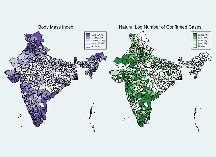
Figure 1. BMI and Natural Log Number of Confirmed Cases at the District-level

Notes: Figures present average values of BMI at the district-level from 2015-2016, and average values of natural log number of Covid19 cases at the district-level as of
April 2020. The pair-wise correlation coefficient between BMI and log number of confirmed cases in the adult sample is 0.072 with p-value < 0.05.
 25

Table 1 – Summary statistics
 Adults (15-54) Women (15-49) Men (15-54) Diff.
Variable Mean SD Mean SD Mean SD
 (1) (2) (3) (4) (5) (6) (7)
Outcomes
Hotspot district 0.318 0.466 0.316 0.465 0.332 0.471 ***
Natural log number of confirmed cases 2.979 1.637 2.966 1.635 3.058 1.649 ***
Case fatality rate 0.433 0.439 0.435 0.440 0.421 0.433 ***
Red zone 0.305 0.444 0.304 0.444 0.311 0.445 ***
Individual level controls
Body mass index 21.849 4.253 21.845 4.311 21.878 3.871 ***
Overweight/obese 0.200 0.400 0.201 0.401 0.191 0.393 ***
Altitude adjusted hemoglobin level 11.966 1.845 11.638 1.623 14.040 1.818 ***
(g/dl)
Glucose level is greater than median 0.497 0.500 0.492 0.500 0.529 0.499 ***
value
Told has high blood pressure on two or 0.088 0.283 0.090 0.287 0.071 0.256 ***
more occasions by doctor or health
professional
Height in centimeters 153.511 7.442 151.927 6.104 163.560 7.307 ***
Age in years 30.146 9.964 29.885 9.751 31.799 11.081 ***
Male 0.136 0.343 0.000 0.000 1.000 0.000
Married 0.721 0.448 0.734 0.442 0.639 0.480 ***
Not educated 0.246 0.431 0.265 0.442 0.125 0.331 ***
Has some or all primary school 0.134 0.340 0.135 0.341 0.128 0.334 ***
Has some secondary school 0.399 0.490 0.389 0.488 0.461 0.498 ***
Completed secondary school or higher 0.221 0.415 0.211 0.408 0.286 0.452 ***
Number of children below 5 years 0.584 0.898 0.591 0.902 0.537 0.871 ***
Hindu 0.804 0.397 0.803 0.398 0.814 0.389
Muslim 0.139 0.346 0.141 0.348 0.130 0.336
Christian 0.024 0.152 0.024 0.152 0.024 0.153 ***
Scheduled tribe 0.095 0.294 0.095 0.294 0.095 0.293
Scheduled caste 0.215 0.411 0.216 0.411 0.210 0.407
Other backward caste 0.450 0.497 0.449 0.497 0.453 0.498
Fuel for cooking: electricity or other 0.007 0.083 0.007 0.082 0.009 0.094 ***
Fuel for cooking: lpg, natural gas, 0.421 0.494 0.418 0.493 0.441 0.497 ***
biogas
Fuel for cooking: kerosene, coal, 0.572 0.495 0.575 0.494 0.550 0.498 ***
lignite, charcoal, wood,
straw/shrubs/grass, ag crop, animal
dung
Food is cooked in a separate building, 0.187 0.390 0.187 0.390 0.185 0.388 ***
outdoors, other
Radio 0.085 0.279 0.085 0.279 0.088 0.283 ***
TV 0.686 0.464 0.682 0.466 0.708 0.455 ***
Fridge 0.313 0.464 0.310 0.463 0.332 0.471 ***
Bicycle 0.576 0.494 0.577 0.494 0.570 0.495 ***
Motorcycle 0.420 0.494 0.414 0.493 0.456 0.498 ***
Car 0.060 0.238 0.059 0.237 0.066 0.249 ***

 26