Stock Price Prediction using Deep Learning - SJSU ScholarWorks
←
→
Page content transcription
If your browser does not render page correctly, please read the page content below
San Jose State University
SJSU ScholarWorks
Master's Projects                                                                                Master's Theses and Graduate Research

Spring 2018

Stock Price Prediction using Deep Learning
Abhinav Tipirisetty
San Jose State University

Follow this and additional works at: http://scholarworks.sjsu.edu/etd_projects
     Part of the Computer Sciences Commons

Recommended Citation
Tipirisetty, Abhinav, "Stock Price Prediction using Deep Learning" (2018). Master's Projects. 636.
http://scholarworks.sjsu.edu/etd_projects/636

This Master's Project is brought to you for free and open access by the Master's Theses and Graduate Research at SJSU ScholarWorks. It has been
accepted for inclusion in Master's Projects by an authorized administrator of SJSU ScholarWorks. For more information, please contact
scholarworks@sjsu.edu.
STOCK PRICE PREDICTION USING DEEP LEARNING

                             Stock Price Prediction using Deep Learning

                                               A Project Report

                                                 Presented to

                                               Dr. Robert Chun

                                    Department of Computer Science

                                         San Jose State University

                                             In Partial Fulfillment

                                     Of the requirements for the class

                                                    CS 298

                                                      By

                                             Abhinav Tipirisetty

                                                  May 2018

                                                       I
STOCK PRICE PREDICTION USING DEEP LEARNING

                                           © 2018
                                      Abhinav Tipirisetty
                                   ALL RIGHTS RESERVED

                                                II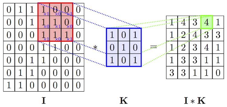
STOCK PRICE PREDICTION USING DEEP LEARNING

            The Designated Thesis Committee Approves the Thesis Titled

              STOCK PRICE PREDICTION USING DEEP LEARNING

                                               by
                                        Abhinav Tipirisetty

      APPROVED FOR THE DEPARTMENTS OF COMPUTER SCIENCE

                              SAN JOSÉ STATE UNIVERSITY

                                             May 2018

                    Dr. Robert Chun Department of Computer Science

                  Dr. Thomas Austin Department of Computer Science

                           Vaishampayan Reddy Pathuri eBay Inc.

                                                   III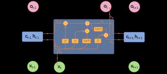
STOCK PRICE PREDICTION USING DEEP LEARNING

                                                    Abstract

       Stock price prediction is one among the complex machine learning problems. It depends

on a large number of factors which contribute to changes in the supply and demand. This paper

presents the technical analysis of the various strategies proposed in the past, for predicting the

price of a stock, and evaluation of a novel approach for the same. Stock prices are represented as

time series data and neural networks are trained to learn the patterns from trends. Along with the

numerical analysis of the stock trend, this research also considers the textual analysis of it by

analyzing the public sentiment from online news sources and blogs. Utilizing both this

information, a merged hybrid model is built which can predict the stock trend more accurately.

                                                       IV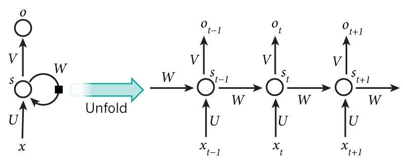
STOCK PRICE PREDICTION USING DEEP LEARNING

                                                    Acknowledgements

       I am grateful and take this opportunity to sincerely thank my thesis advisor, Dr. Robert

Chun, for his constant support, invaluable guidance, and encouragement. His work ethic and

constant endeavor to achieve perfection have been a great source of inspiration.

       I wish to extend my sincere thanks to Dr. Thomas Austin and Mr. Vaishampayan Reddy

Pathuri for consenting to be on my defense committee and for providing invaluable suggestions to

my project without which this project would not have been successful.

       I also would like to thank my friends and family, for their support and encouragement

throughout my graduation.

                                                           V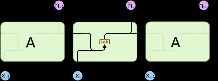
STOCK PRICE PREDICTION USING DEEP LEARNING

Table of Contents

Abstract .................................................................................................................... IV

Acknowledgements .................................................................................................... V

List of tables ............................................................................................................... 3

List of figures.............................................................................................................. 4

Chapter 1 ................................................................................................................... 5

   1.1 Introduction .................................................................................................................5

   1.2 Motivation ...................................................................................................................6

Chapter 2 ................................................................................................................... 8

   2.1 Background ..................................................................................................................8

       2.1.1 Supervised Learning ....................................................................................................... 8

       2.1.2 Unsupervised Learning ................................................................................................... 9

       2.1.3 Support Vector Machines............................................................................................... 9

       2.1.4 Deep Learning and Artificial Neural Networks ............................................................. 10

       2.1.5 Recurrent Neural Network ........................................................................................... 11

       2.1.6 Long-short term memory ............................................................................................. 12

   2.2 Related Work ............................................................................................................. 14

       2.2.1 Using stacked auto encoders (SAEs) and long short-term memory (LSTM) ................ 14

       2.2.2 Integrating Text Mining Approach using Real-Time News: .......................................... 15

       2.2.3 Stock Price Prediction using Linear Regression based on Sentiment Analysis ............ 15

                                                                   1
STOCK PRICE PREDICTION USING DEEP LEARNING
2.3 Limitations of existing models .................................................................................... 16
Chapter 3 ................................................................................................................. 17
Proposed Approach.......................................................................................................... 17
3.1 Numerical Analysis ..................................................................................................... 17
Implementation: ................................................................................................................... 22
Normalization: ....................................................................................................................... 23
3.2 Textual Analysis ......................................................................................................... 25
Machine Learning Model – Approach 1 - SVM: .................................................................... 26
Machine Learning Model – Approach 2 - LSTM: ................................................................... 27
3.4 Merged Model ........................................................................................................... 32
Chapter 4 ................................................................................................................. 34
4.1 Metrics ...................................................................................................................... 34
Mean Squared Error: ............................................................................................................. 34
Accuracy: ............................................................................................................................... 34
4.1 Experiments on Base Model ....................................................................................... 35
4.2 Experiments on Numerical analysis ............................................................................. 37
4.3 Experiments on Textual Analysis: ................................................................................ 40
4.4 Experiments on Merged Model ................................................................................... 45
Chapter 5 ................................................................................................................. 49
Conclusion and Future Work ............................................................................................ 49
References ............................................................................................................... 50
2STOCK PRICE PREDICTION USING DEEP LEARNING
List of tables
Table 1 Sample news headlines and their influence on stock price ................................. 25
Table 2 SVM model results for prediction using Tech news and Company only news ... 44
Table 3 LSTM model results for prediction using Tech news and Company only news . 45
3STOCK PRICE PREDICTION USING DEEP LEARNING
List of figures
Figure 1 showing the data points represented in a 2D space and the support vector [5] .... 9
Figure 2 Feed Forward Neural Network [7] ..................................................................... 11
Figure 3 Unfolded basic recurrent neural network. [8]..................................................... 12
Figure 4 Simple structure of RNNs looping module. [11]................................................ 13
Figure 5 Long short-term memory unit [12] ..................................................................... 13
Figure 6 Sliding window learning the trends in stock price [21] ...................................... 18
Figure 7 Unrolled version of the network for Numerical Analysis .................................. 19
Figure 8 LSTM network architecture for textual analysis ................................................ 27
Figure 9 Convolution of input vector I using filter K [22] ............................................... 29
Figure 10 Convolutional Neural Network for Image Classification [24] ......................... 29
Figure 11 Convolution of single dimensional vector input [25] ....................................... 30
Figure 12 SVM with RBF kernel with Window Size 10 .................................................. 36
Figure 13 SVM with RBF kernel with Window Size 15 ................................................. 36
Figure 14 GOOG LSTM 32 InputSize 1........................................................................... 38
Figure 15 GOOG lstm size = 128 and input size = 1 ........................................................ 39
Figure 16 input_size=5, lstm_size=128 and max_epoch=75 ............................................ 40
Figure 17 News probabilities aligned with same day’s prices .......................................... 46
Figure 18 News probabilities aligned with prices 1 day ahead ........................................ 47
Figure 19 Comparison of predictions without news and with news ................................. 48
Figure 20 Comparison of predictions with baseline model and proposed model ............. 48
4STOCK PRICE PREDICTION USING DEEP LEARNING
Chapter 1
1.1 Introduction
Stock price is the price of a single stock among the number of stocks sold by a company
listed in public offering. Having stocks of a public company allows you to own a portion of it.
Original owners of the company initially sell the stocks to get additional investment to help the
company grow. This initial offering of stocks to the public is called Initial Public Offering (IPO).
Stock prices change because of the supply and demand. Suppose, if many people are
willing to buy a stock, then the price goes up as there is more demand. If more people are willing
to sell the stock, the price goes down as there is more supply than the demand. Though
understanding supply and the demand is relatively easy, it is hard to derive what factors exactly
contribute to the increase in demand or supply. These factors would generally boil down to socio-
economic factors like market behavior, inflation, trends and more importantly, what is positive
about the company in the news and what’s negative.
Predicting the accurate stock price has been the aim of investors ever since the beginning
of the stock market. Millions of dollars worth of trading happens every single day, and every trader
hopes to earn profit from his/her investments. Investors who can make right buy and sell decisions
will end up in profits. To make right decisions, investors have to judge based on technical analysis,
such as company’s charts, stock market indices and information from newspapers and microblogs.
However, it is difficult for investors to analyze and forecast the market by churning all this
information. Therefore, to predict the trends automatically, many Artificial Intelligence (AI)
techniques have been investigated [1] [2] [3]. Some of the first research in prediction of stock
prices dates back to 1994, in which a comparative study [4] with machine learning regression
5STOCK PRICE PREDICTION USING DEEP LEARNING
models was performed. Since then, many researchers were investing resources to devise strategies
for forecasting the price of the stock.
1.2 Motivation
Efficient Market Hypothesis is one of the popular theories in financial economics. Prices
of the securities reflect all the information that is already available and it is impossible to
outperform the market consistently. There are three variants of Efficient Market Hypothesis
(EMH); namely weak form, semi-strong form and the strong form. Weak form states that the
securities reflect all the information that is publicly available in the past. Semi Strong form states
that the price reflects all the publicly available data and also, they change instantly to reflect the
newly available information. The strong form would include even the insider or private
information.
But this theory is often disputed and highly controversial. The best example would be
investors such as Warren Buffet, who have earned huge profits over long period of time by
consistently outperforming the market. Even though predicting the trend of the stock price by
manually interpreting the chaotic market data is a tedious task, with the advent of artificial
intelligence, big data and increased computational capabilities, automated methods of
forecasting the stock prices are becoming feasible. Machine learning models are capable of
learning a function by looking at the data without explicitly being programmed. But
unfortunately, the time series of a stock is not a function that can be easily mapped. It can be
best described more as a random walk, which makes the feature engineering and prediction much
harder. With Deep Learning, a branch of machine learning, one can start training using the raw
data and the features will be automatically created when neural network learns. Deep Learning
6STOCK PRICE PREDICTION USING DEEP LEARNING
techniques are among those popular methods that have been employed, to identify the stock trend
from large amounts of data but until now there is no such algorithm or model which could
consistently predict the price of future stock value correctly. Lot of research is going on both in
academia and industry on this challenging problem.
7STOCK PRICE PREDICTION USING DEEP LEARNING
Chapter 2
2.1 Background
This section will explain what machine learning is and popular algorithms used by previous
researchers to predict stock prices. This will also provide a background of the technologies we use
as part of this research.
Machine Learning is a field of Computer Science that gives Computers the ability to learn.
There are two main categories of machine learning algorithms. They are Supervised Learning and
Unsupervised Learning. The process of training a machine learning model involves providing an
algorithm and the data so that model learns its parameters from the provided training data.
2.1.1 Supervised Learning
In supervised learning, we train the machine learning algorithm with a set of input
examples and their associated labels. The model tries to approximate the function y = f(x) as close
as possible, where x is the input example and y is its label. As we are using a training dataset with
correct labels to teach the algorithm, this is called a supervised learning. Supervised learning
algorithms are further grouped into regression and classification, based on the output variable. If
the output variable is a continuous variable, it is called a regression task. Predicting house price,
stock price are examples of regression tasks. If the output variable is categorical variable like color,
shape type, etc. it is called a classification task.
In practice, majority of the machine learning applications use supervised learning
algorithms. Logistic regression, linear regression, support vector machines and random forests are
examples of supervised learning algorithms.
8STOCK PRICE PREDICTION USING DEEP LEARNING
2.1.2 Unsupervised Learning
In Unsupervised learning, we train the machine learning algorithm with only the input
examples but no output labels. The algorithm tries to learn the underlying structure of the input
examples and discover patterns. Unsupervised learning algorithms can be further categorized
based on two tasks, namely Clustering and Association. In clustering, an algorithm like k-means
tries to discover inherent clusters or groups in the data. In association rule mining, algorithms like
apriority tries to predict the future purchase behaviors of customers.
2.1.3 Support Vector Machines
SVM belongs to the class of supervised algorithms in machine learning, which relies on
statistics. It can be used for both regression and classification tasks. In SVM, we plot each point
in the dataset in an n-dimensional space, where each dimension corresponds to a feature. Value of
the data point for that feature will represent the location on the corresponding axis. During training,
SVM separates the set of labeled input examples by an optimal hyperplane. During testing, the
class of the unlabeled data point is determined by plotting it and checking which side the new point
is to the hyperplane.
Figure 1 showing the data points represented in a 2D space and the support vector [5]
9STOCK PRICE PREDICTION USING DEEP LEARNING
Lin et al. [6] proposed a stock market forecast system based on SVM. This model is capable
of choosing a decent subset of features, controlling over fitting and assessing stock indicator. This
research is based on the stock market datasets of Taiwan and this model resulted in better
performance than the traditional forecast system.
A significant problem while using SVM is that, the input variables may lie in a very high
dimensional space. Especially when the dimensions of the features ranges from hundreds to
thousands, training the model requires huge computation and memory.
2.1.4 Deep Learning and Artificial Neural Networks
Deep learning is part of a broader family of ML methods based on learning data
representations, as opposed to task specific algorithms. Deep learning models use a cascade of
multi layered non-linear processing units called as neurons, which can perform feature extraction
and transformation automatically. The network of such neurons is called an Artificial Neural
Network.
Artificial Neural Networks(ANN) are an example for non-parametric representation of
information in which the outcome is a nonlinear function of the input variables. ANN is an
interconnected group of nodes which simulate the structure of neurons present in the human brain.
These neurons are organized in the form of consecutive layers, where output of the current layer
of neurons is passed to the successive layer as the input. If the interconnections between the layers
of neurons do not form a cycle, that neural network is called a feed forward neural network. In a
feed forward neural network, each layer applies a function on the previous layer’s output. The
hidden layer transforms its inputs into something that output layer can use and the output layer
applies activations on its inputs for final predictions.
10STOCK PRICE PREDICTION USING DEEP LEARNING
Figure 2 Feed Forward Neural Network [7]
2.1.5 Recurrent Neural Network
Recurrent Neural Network (RNN) is a class of ANN in which connections between the
neurons form a directed graph, or in simpler words, having a self-loop in the hidden layers. This
helps RNNs to utilize the previous state of the hidden neurons to learn current state. Along with
the current input example, RNNs take the information they have learnt previously in time. They
use internal state or memory to learn sequential information. This enables them to learn a variety
of tasks such as handwriting recognition, speech recognition, etc.
In a traditional neural net, all input vector units are assumed to be independent. As a result,
sequential information cannot be made use of in the traditional neural network. But whereas in the
RNN model, sequential data of the time series generates a hidden state and is added with the output
of network dependent on hidden state. As the stock trends are an example of a time series data,
this use case is a best fit for RNNs. The following figure shows an RNN model expanded into a
complete network.
11STOCK PRICE PREDICTION USING DEEP LEARNING
Figure 3 Unfolded basic recurrent neural network. [8]
Based on the outcome of the output layer, updates to the weights of hidden layers are
propagated back. But in deep neural networks, this change will be vanishingly small to the layers
in the beginning, preventing the weights to change its value and stopping the network to learn
further. This is called vanishing gradient problem [9].
2.1.6 Long-short term memory
Long short-term memory (LSTM) is a type of recurrent neural-network architecture in which
the vanishing gradient problem is solved. LSTMs are capable of learning very long-term
dependencies and they work tremendously well on a large variety of problems. LSTMs are first
introduced by Hochreiter et al. in 1997 [10]. In addition to the original authors, many researchers
contributed to the architecture of modern LSTM cells.
Recurrent neural networks are generally designed in a chain like structure, looping back to the
previous layers. In standard RNNs, this looping module will have a very simple structure, as shown
in the Figure 4. This structure can be a simple tanh layer controlling the flow.
12STOCK PRICE PREDICTION USING DEEP LEARNING
Figure 4 Simple structure of RNNs looping module. [11]
Whereas in LSTMs, instead of this simple structure, they have four network layers interacting
in a special way. General architecture of LSTMs is shown in Figure 5. Normally LSTM’s are
augmented by gates called “forget” gates. By controlling these gates, errors can be backpropagated
through any number of virtual layers. This mechanism enables the network to learn tasks that
depend on events that occurred millions of time steps ago.
Figure 5 Long short-term memory unit [12]
13STOCK PRICE PREDICTION USING DEEP LEARNING
2.2 Related Work
Mining time series data and the information from textual documents is currently an
emerging topic in the data mining society. Increasingly many researchers are focusing their studies
on this topic [13], [14], [15]. Currently, many of the approaches deal with a single time series. The
relationships between different stocks and influences they can have on one another are often
ignored. However, this is valuable information. For example, if the price of Honda’s stocks goes
down, that may trigger a movement of stock prices of Toyota.
Number of researchers published papers in the last decade on different strategies. Two
interesting approaches dealing with mining the information from news and forecasting future stock
price were considered. These approaches are briefly explained in the following sections.
2.2.1 Using stacked auto encoders (SAEs) and long short-term memory (LSTM)
Wei Bao, et al. [16] presented a novel deep learning framework where stacked auto
encoders, long-short term and wavelet transforms (WT) are together used for stock price
prediction. The SAEs for the deep features which are extracted hierarchically is introduced in
forecasting the stock price in this paper for the first time. This deep learning framework consists
of 3 stages. Firstly, WT decomposes the time series of the stock price to eliminate noise. Then, for
generation of deep high-level features, SAEs are applied for stock price prediction. Lastly, high-
level denoising features are fed into long short-term memory to predict closing price of the next
day. Performance of the proposed model is examined by choosing 6 market indices and their
corresponding features. In both predictive accuracy and profitability performance, this approach
had claimed to outperform other similar models.
14STOCK PRICE PREDICTION USING DEEP LEARNING
2.2.2 Integrating Text Mining Approach using Real-Time News:
News is a very important factor which effects the stock prices. A positive article about a
company’s increased sales may directly correlate with the increase in its stock price, and vice-
versa. A novel approach for mining text from real time news and thus predicting the stock prices
was proposed in the paper by Pui Cheong Fung, et al [17] . Mining textual information from the
documents and time series simultaneously is a topic of raising interest in data mining community.
There is a consistent increase in the number of researches conducted in this area [18] [14]. In this
paper, a new approach is proposed for multiple time series mining. It involves three procedures as
follows: 1) discovery of potentially related stocks; 2) selection of stocks; and 3) alignment of
articles from different time series.
2.2.3 Stock Price Prediction using Linear Regression based on Sentiment Analysis
In 2015, Yahya, et al. [19] tried to utilize the sentiment of the posts from social media
websites like twitter to predict the stock prices in Indonesian Stock Market. They used naïve Bayes,
support vector machines and random forest algorithms to classify tweets about companies and
compared the results of the different algorithms. They claimed that the random forest model had
achieved best performance among the 3 algorithms with 60.39% accuracy. Naïve Bayes stood as
the second-best model with 56.50% accuracy. Then they have used supervised classification
algorithms such as SVM, Decision Trees and linear regression as predictive models and attempted
to predict price fluctuation and margin percentage. A comparative analysis was performed on the
results of all the models.
15STOCK PRICE PREDICTION USING DEEP LEARNING
2.3 Limitations of existing models
While most of the previous research in this field were concentrating on techniques to
forecast stock price based on the historical numerical data such as past stock trends, there is not
much research put into the textual analysis side of it. News and media has huge influence on human
beings and the decisions we take. Also, fluctuations in the stock market are a result of the trading
activities of human beings. As news articles influence our decisions and as our decisions influence
the market, the news indirectly influence the stock market. Therefore, extracting information from
news articles may yield better results in predicting the stock prices. News sensitive stock trend
prediction [14], sentiment polarity analysis using a cohesion based approach [20], mining of text
concurrent text and time series [15] are some of the distinguished works in the domain.
However, there are few issues in the above-mentioned works. First being many of these
researches used Bag of Words (BoW) approach to extract information from the news reports,
despite of the fact that the BoW approach cannot capture some important linguistic characteristics
such as word ordering, synonyms and variant identification. Next, most works either used just the
numerical information or textual information, whereas the market analysts used both. Also,
previous approaches did not consider the fact that the stock prices between the companies is
correlational. Finally, the approaches which used textual information to forecast, did not consider
stock prices as time series.
16STOCK PRICE PREDICTION USING DEEP LEARNING
Chapter 3
Proposed Approach
In this research we perform both numerical analysis and the textual analysis on the stocks
and news dataset to try predicting the future price of the stock. Numerical analysis will be
performed by treating the stock trend as a time series and we try to forecast future prices by
observing the prices over last x number of days. In textual analysis we perform sentiment analysis
of the news articles and learn the influences of news on stock prices. Finally, predictions from
these two models will be used as input to a merged model to output final predictions.
3.1 Numerical Analysis
Numerical analysis aims at building a recurrent neural network based model to predict the
stock prices of S&P500 index. RNNs are good at learning and predicting time series data. As stock
market data is a time series, RNNs are best suitable for this task. For this purpose, we use a specific
type of RNNs called as Long Short-Term Memory. As explained in Chapter 2 – Background
section, LSTM is specially designed cell which can help the network to memorize long term
dependencies. In numerical analysis, we try to learn the patterns and trends of stock prices over
the past, and this information will be augmented by the textual information later.
S&P 500 index data from 3rd January 1950 until 31st December 2017 downloaded from
Yahoo! Finance GSPC is used for this purpose. To simplify the problem, we use only the closing
prices of the stock index. Stock prices are a time series data of length N. We choose a sliding
window w of variable size, which moves step by step from the beginning of the time series. Figure
6 illustrates the sliding window wt which is used as the input to predict wt+1.
17STOCK PRICE PREDICTION USING DEEP LEARNING
Figure 6 Sliding window learning the trends in stock price [21]
While moving the sliding window, we move it to the right by the window size so that there
is no overlap between the previous window and the current window. Each input window at each
step is passed to a LSTM cell which acts as the hidden layer. This layer would predict values of
the next window. While predicting the prices for window Wt+1, we use values from the first sliding
window W0 until the current time Wt, where t is the time.
W0 = (p0,p1,…,pw−1)
W1=(pw,pw+1,…,p2w−1)
Wt=(ptw,ptw+1,…,p(t+1)w−1)
The function we are trying to predict is:
f(W0,W1,…,Wt) ≈ Wt+1
18STOCK PRICE PREDICTION USING DEEP LEARNING
The output window Wt+1:
Wt+1=(p(t+1)w,p(t+1)w+1,…,p(t+2)w−1)
Figure 7 Unrolled version of the network for Numerical Analysis
During the training process, predicted output is calculated by using the randomly assigned
weights and compared with the actual value. Error is calculated at the output layer and it is
propagated back through the network. This is called back propagation and as this is applied to a
timeseries like data as in our case, we call it Back Propagation Through Time (BPTT). During
backpropagation, we update weights to minimize the loss in the next step. To update the weights,
we calculate the gradient of the weight by multiplying weight’s delta and input activations then
subtract a ratio of this gradient from the weight. This ratio would influence the quality and speed
of the training. This ratio is called Learning Rate. If the learning rate is set high, the network learns
fast but the learning will be more accurate when the learning rate is low. Learning process is
repeated until the accuracy or loss meets a threshold.
19STOCK PRICE PREDICTION USING DEEP LEARNING
By the design of RNNs, they depend on arbitrarily distant inputs. Due to this,
backpropagation to the layers very far away requires heavy computational power and memory. In
order to make the learning feasible, the network is unrolled first so that it contains only a fixed
number of layers. The unrolled version of the recurrent neural network is illustrated by Figure 7
Unrolled version of the network for Numerical Analysis. The model is then trained on that finite
approximation of the network.
During training, we feed inputs of length n at each step and then perform a backward pass.
This is done by splitting the sequence of stock prices into non-overlapping small windows. Each
window will contain “s” numbers. Each number is one input element and “n” consecutive such
elements are grouped to form a training input.
For example, if s=2 and n=3, the training example will be as follows.
Input1 = [[p0, p1], [p2, p3], [p4, p5]], Label1 = [p6, p7]
Input2 = [[p2, p3], [p4, p5], [p6, p7]], Label2 = [p8, p9]
Input3 = [[p4, p5], [p6, p7], [p8, p9]], Label3 = [p10, p11]
Where p is the stock price at a single instance of time.
Dropout parameter:
Deep neural networks with many parameters are powerful systems to learn most of the
complex tasks. However, they suffer from the problem of overfitting. The problem is that generally
the available data will be limited and in most cases, it will not be sufficient enough to learn
complex patterns in the data. As the underlying patterns between inputs and the output can only
be mapped using a non-linear approximation function, the hidden layers tend to fit a higher order
function to accurately map the outputs. By doing so, they perform best during training but fail
miserably during testing. Therefore, we use regularization techniques to avoid overfitting. In
20STOCK PRICE PREDICTION USING DEEP LEARNING
general machine learning algorithms, regularization is achieved by using a penalty to the loss
function or combining the results from different models and then averaging it. But neural networks
are more complex and as they require comparatively higher computational resources, model
averaging is not a solution. Therefore, we use a technique called dropout, in which we randomly
drop a few units from the network during training, thus preventing co-adaptation between the units.
We use the dropout technique in our model to avoid overfitting. The model will have a
configurable number of LSTM layers (n) stacked on top of each other and in each layer, there are
a configurable number of LSTM cells (l). Then there is a dropout mask with a configurable
percentage (d) of number of cells to be dropped during the dropout operation. We calculate the
keep probability (k) from d, which is basically derived from the below equation
k=1–d
The training process takes place by cycling over the data multiple times. Each full pass
over all the data points is called an epoch. In total, training requires m number of epochs over the
data. In each epoch, the data is split into b sized groups called mini-batches. In one Back
Propagation Through Time learning, we pass one mini batch of data as input to the model for
training. After each step, we update the weights at a rate defined by the configurable parameter
“l”, which represents learning rate. As explained earlier, higher learning rate lets the network to
train faster, but to achieve better accuracy, we need a lower learning rate. In order to find an optimal
value, initially we set learning rate to a higher value and at each succeeding epoch it decays by
multiplying it with a value defined by “d” (stands for learning rate decay).
21STOCK PRICE PREDICTION USING DEEP LEARNING
Implementation:
We used tensorflow library to model the network. We first define the placeholders for
inputs and targets as follows.
inputs = tf.placeholder(tf.float32, [None, n, s])
targets = tf.placeholder(tf.float32, [None, s])
learning_rate = tf.placeholder(tf.float32, None)
We create the LSTM cell and wrap it with a dropout wrapper to avoid overfitting of the
network to the training dataset.
def _create_one_cell():
lstm_cell = tf.contrib.rnn.LSTMCell(l, state_is_tuple=True)
lstm_cell = tf.contrib.rnn.DropoutWrapper(lstm_cell, output_keep_prob=k)
return lstm_cell
Number of layers of LSTM cells in the network are configurable. This will be passed as an
input to the program. When multiple LSTM cells are used, we try to stack them using the
tensorflow’s MultiRNNCell class. This class helps in connecting multiple LSTM cells sequentially
into one composite cell.
cell = tf.contrib.rnn.MultiRNNCell( [_create_one_cell() for _ in range(l)],
state_is_tuple=True)
The Dynamic RNN class present in the TensorFlow library will create the RNN specified
by the RNNCell created in previous step.
val, _ = tf.nn.dynamic_rnn(cell, inputs, dtype=tf.float32)
The last column of the result of above dynamic RNN is then multiplied with weight and
bias is added to get the prediction of this step.
22STOCK PRICE PREDICTION USING DEEP LEARNING
prediction = tf.matmul(last, weight) + bias
Loss is calculated by squaring the difference between the predicted value and the true
value, then finding the mean of the result.
Where Yi is the vector representing actual values of the stocks and Y^i is the vector
representing predicted stock values. We use RMSProp optimization algorithm to perform gradient
descent. Learning rate is passed as a parameter to the RMSPropOptimizer and this learning rate
will be gradually decayed by the decay parameter in each epoch. After training for the specified
number of epoch, the training stops.
Normalization:
At each step, latest 10% of the data is used for testing and as the S&P 500 index gradually
increases over time, test set would have most of the values larger than the values of training set.
Therefore, values which are never seen before are to be predicted by the model. Following figure
shows such predictions.
23STOCK PRICE PREDICTION USING DEEP LEARNING
We can see from the above figure that the predictions are worse for new data. Therefore,
we normalize the values by the last value in the previous window, thus we will be predicting
relative changes in the prices instead of the absolute values. Following is the equation for
normalizing the values in a window. W’t is the normalized window and t is the time.
Above figure shows that after normalization, model is able to predict better for new data.
24STOCK PRICE PREDICTION USING DEEP LEARNING
3.2 Textual Analysis
In textual analysis, we analyze the influence of news articles on stock prices. For this
purpose, news articles from websites like reddit were downloaded, and sentiment of the headlines
was calculated. Then we tried to correlate them with the stock trend to find their influence on the
market. Even though sentiment can reveal whether the news is positive or negative, it is hard to
know how much it would affect the stock price. Therefore, the problem of predicting the exact
stock price was simplified to problem of predicting whether the stock price rises or falls, by
transforming the values of close price column to Boolean having values 0 or 1. A value of “1”
denotes that the price increased or stayed the same, whereas “0” indicates that the price reduced.
Following are some of the examples of news headlines which influenced the stock prices.
Date Headline Influence
2014-03-19 A Surprising Number of Places Have Banned Google Glass In Negative
San Francisco
2014-03-20 Lawsuit Alleges That Google Has Crossed A 'Creepy Line' Negative
2014-05-02 Google to Acquire Favorite Live Streaming Service Twitch for Positive
$1B
2014-05-21 Google overtakes Apple as Most Valuable Global Brand Positive
2014-05-22 Google Inc (GOOGL) Plans to Spend $30 Billion On Foreign Positive
Acquisitions
2014-06-19 Heads up: Hangouts is being weird today (other Google services Negative
too)
2014-07-09 Google Co-Founders Talk Artificial Intelligence Just a Matter Positive
of Time
Table 1 Sample news headlines and their influence on stock price
Then this vector was passed to machine learning algorithms to find mapping between
sentiment values and output trends.
25STOCK PRICE PREDICTION USING DEEP LEARNING
We have the following research problems at this stage.
1. What machine learning algorithms perform best in learning the correlation between
news and stock trend?
2. Does the news about other companies in the same field have influence on the stock
prices of a company?
3. How many days would it take for the published news to influence the market?
For research problem 1, we chose two approaches as discussed below.
Machine Learning Model – Approach 1 - SVM:
In the first approach, we calculated sentiment of the news articles and used a machine
learning model like Support Vector Machines to find the mapping between sentiment vector and
stock trends. To calculate the sentiment, we have used Valence Aware Dictionary and Sentiment
Reasoner (VADER) which is a lexicon and sentiment intensity analyzer specially tuned to
sentiments expressed in social media. As the headline of a news article can provide enough context
to analyze the sentiment, we ignore the body of the article and consider only the headline for
analysis. For each headline, sentiment polarity and intensity is calculated using VADER algorithm,
which returns a value from 0 to 1 to represent a positive polarity and the magnitude represents the
intensity, and returns a value from 0 to -1 to represent negative polarity. 0 can be treated as neutral
sentiment. A vector is created using these sentiment values and this vector is passed as the input
to the SVM model for training, whereas the target is a boolean vector representing rise or fall of
stock price.
26STOCK PRICE PREDICTION USING DEEP LEARNING
Machine Learning Model – Approach 2 - LSTM:
In this approach, recurrent neural networks were used to map the function between
sentiment values and the target price. Specifically, we used Long Short-Term Memory network as
they were proven to be successful with text data. As the target variable we are predicting is either
0 or 1, this would be a classification problem. Therefore, architecture of the neural network is
designed in such a way that it outputs a fully connected layer with softmax or sigmoid activation
function.
Architecture of the LSTM network is illustrated by the Figure 8 LSTM network
architecture for textual analysis.
Figure 8 LSTM network architecture for textual analysis
Network:
Input:
The news headlines are first preprocessed and passed as inputs to the neural network.
During preprocessing, all non-alphabetical characters were removed and rest of the characters were
decapitalized. Next word embeddings are calculated.
Word Embeddings:
In NLP, word embeddings is a technique of representing words as vectors of real numbers
in which words with similar meanings will have similar representation. This is one of the key
breakthroughs in deep learning that achieved impressive performance for NLP problems.
27STOCK PRICE PREDICTION USING DEEP LEARNING
Words are represented in a distributed vector space based on their usage, and therefore words
which are used similarly will have similar representation. First tokenizer takes the input words and
indexes the text corpus based on word count, term frequency inverse document frequency (TF-
IDF). For indexing we store a maximum of 2000 words in the corpus. Therefore, the words which
are not present in top 2000 will have the index set to 0. The headlines are transformed into vectors
of fixed size of 100. If the headline is shorter than 100 words, zeros are padded to it. Then, these
vectors are passed to an Embedding Layer in the neural network.
Convolutional Layer:
A convolutional layer consists of a set of filters whose weights are learnt during the training
process. Dimensions of the filter are spatially smaller than the input vector’s dimensions but will
have the same depth. During a forward pass, the filters are slid over the width and height of the
input vector and dot product is calculated between the values of the filter and the input at each
position. The convolution process is shown in Figure 9, where I is the input vector and K is the
filter. During the training process, network will learn these filters that activate when they see the
target concealed in the input.
28STOCK PRICE PREDICTION USING DEEP LEARNING
Figure 9 Convolution of input vector I using filter K [22]
As we know convolutional layers are generally used for images as they are suitable for matrix
representations. But as embedding vectors are also matrix representations of words, convolutional
layers can be applied to word embeddings [23]. As images are more meaningful as a 2-dimensional
representation than one dimensional array like representation, 2D convolution layer is used for
images and for videos a 3D convolution layer is used. But in case of sentences (or words), a single
dimension makes more sense than 2D or 3D. Therefore a 1-dimensional convolution layer is used
for processing textual information.
Figure 10 Convolutional Neural Network for Image Classification [24]
29STOCK PRICE PREDICTION USING DEEP LEARNING
A typical convolutional neural network for image classification problem is shown in the
Figure 10. In the above example the sliding window (called filter) scans over the image and
transforms pixel information into a vector or matrix representation. Similarly, for sentences we
use 1 dimensional layer as shown in Figure 11.
In convolutional layers, a window or typically called as a filter, will be sliding over the
input vector, at each step calculating convolution of the filter over data. To reflect the word
negations, filter should consider the surrounding words to the current word. Therefore, we chose
a kernel size of 3, so that word negations are accounted in the weights.
Figure 11 Convolution of single dimensional vector input [25]
30STOCK PRICE PREDICTION USING DEEP LEARNING
Max Pool Layers:
Generally, a pooling layer is inserted between successive convolution layers in a convolutional
network architecture. Pooling layer progressively reduces the spatial size of the representation
thereby significantly reducing the number of parameters, computation in the network and
controlling overfitting. Pooling layer is simply a max operation applied on every slice of input
with specified dimension. Since the neighboring values in the convolutions are strongly correlated,
it is understandable to reduce the output size by subsampling the response from filter. It is most
common [26] to use a max pool layer of size 2, as values further apart are less correlated.
LSTM Cell:
Output from the max pool layer is passed as the input to the LSTM cell. LSTM cell will have 3
main parameters to be set. They are number of units, activation function and recurrent activation
function. Number of units is found by cross validation. Recurrent activation is applied to inputs,
forget gate and the output gates, whereas the activation is applied to candidate hidden state and the
output hidden state. Default values for recurrent activation function is a hard-sigmoid function and
for activation function default value is hyperbolic tangent function.
Output Layer:
As the network output is between 0 and 1, we use a sigmoid activation function in the
output layer.
31STOCK PRICE PREDICTION USING DEEP LEARNING
3.4 Merged Model
Step 1:
Numerical analysis model is capable of analyzing the stock trends from the given input
window, extract patterns out of it and is able to predict the future trend. Whereas the textual
analysis model is trained to get sentiments from the news articles and predict if the stocks would
rise or fall. Therefore, the idea is that merging these two models should give better prediction
results.
To achieve this, we train the numerical analysis model with past couple of months of stock
trends related to a particular company. This model will output the predicted prices P for next p
number of days. Value of p is calculated as follows.
p = size(Input Samples) / (n * s)
where,
n = number of steps in back propagation
s = number of elements in input window
Also, let the actual prices be Y, which will be used later in Step 3.
Step 2:
Next, we train the textual analysis model with historical news related to that particular
company and corresponding stock trends. This model will learn what type of news can trigger a
rise in stock price and what type of news can trigger a fall in stock price. In step 2, news headlines
for each day in P are collected and passed as input to textual analysis model. This will output the
vector with probabilities of rise or fall for each day. Let’s call this vector N.
32STOCK PRICE PREDICTION USING DEEP LEARNING
Step 3:
Now we have the predicted prices vector P, news predictions vector N and the actual prices
vector Y. We will now pass the vectors P and N to an SVM regressor as inputs and Y as the output.
After training SVM will learn how values of N will influence P. Output of this merged model are
the final predictions using both numerical analysis and textual analysis.
33STOCK PRICE PREDICTION USING DEEP LEARNING
Chapter 4
In this chapter we are going to discuss our experiments and results of the models mentioned
until now. We will first go through the metrics we used to evaluate the models and then we will
summarize the experiments on the numerical analysis model, textual analysis and the merged
model.
4.1 Metrics
Mean Squared Error:
Mean Squared Error (MSE) of an estimator measures the average of squares of the errors.
The term error here denotes the difference between the actual value and the estimated value. Below
equation denotes the mathematical equation for calculating the mean squared error.
Here Yi represents the vector of the actual values and Y^i is the vector of predicted values.
MSE is generally used when we have vectors with continuous values. We will be using
this metric for comparing the results of the Numerical Analysis models and the merged model.
Accuracy:
Accuracy of a binary classifier is a statistical measure of how well the classifier is able to
predict the correct values. It is the percentage of true results among total number of samples. It is
denoted by the below equation.
Accuracy = True Positives / Total number of predictions
34STOCK PRICE PREDICTION USING DEEP LEARNING
Accuracy is a metric generally used for classification problems. As in textual analysis, we
converted the problem of predicting exact stock prices to predicting whether the price increased or
decreased, we can use the accuracy as the metric to evaluate the model.
4.1 Experiments on Base Model
We have used SVM regressor implementation from Scikit Learn machine learning library
as the base model for evaluation. Stock prices are split into windows of fixed sizes. At each step
prices in one window are passed as the input to train the model and the next day’s stock price is
passed as the target variable. Therefore, the input vector X will be a 2-dimensional array of n input
samples where each input sample will contain a sequence of stock prices in one window. The
output vector y is a 1-dimensional vector of stock prices where each element in the vector is the
stock price on the day next to corresponding input window. Based on cross validation, we have
chosen Radial Basis Function (RBF) as the kernel to the SVM and input window size of 15.
Following are the predictions with input window size 10 and 15.
35STOCK PRICE PREDICTION USING DEEP LEARNING
Figure 12 SVM with RBF kernel with Window Size 10
Figure 13 SVM with RBF kernel with Window Size 15
36STOCK PRICE PREDICTION USING DEEP LEARNING
Corresponding mean squared error for Window size 10 is 0.000757094 and for Window
size 15, the error is 0.0007262213, therefore the model with window size 15 and RBF kernel is
chosen as base model.
4.2 Experiments on Numerical analysis
In the experiment, we compare the predictions of the LSTM model we designed as part of
numerical analysis. Stock prices data was downloaded from Yahoo Finance for the companies
Microsoft, Apple, Google and IBM. The data contains closing price of the above-mentioned
companies for dates ranging from Sept 1st, 2004 till Dec 31st, 2017. As explained during the
numerical model construction, the dataset will be split into groups where each group will have
input_size number of points. This can be imagined as a sliding window which starts at the
beginning of the dataset and moves forward one group at a time. The model is trained by taking
the current window as the input and tries to predict the values of next window. Therefore, the
prices of the last window can be treated as the test values.
Train / test split:
The data is split in such a way that 90% of the data is always used for training and the latest
10% is used for testing.
First, the model was trained with input size = 1 and lstm size = 32 to begin with. The results
are as shown in the figure below. Mean squared error of this configuration is 0.0006770748.
37STOCK PRICE PREDICTION USING DEEP LEARNING
Figure 14 GOOG LSTM 32 InputSize 1
From the results we can observe that the predictions were not accurate enough to make the
buying decisions.
As lstm size will denote the capacity of the LSTM cell, and depending on the amount of
data, we have to choose an appropriate size. Therefore, we tried to tune the lstm size parameter.
When the model was trained with lstm size = 128 and input size = 1, loss (MSE) is reduced. This
can be observed from the below graph. Mean squared error of this configuration is 0.0006423764.
38STOCK PRICE PREDICTION USING DEEP LEARNING
Figure 15 GOOG lstm size = 128 and input size = 1
Input size is another parameter to be tuned. Number of examples in the training window
can be controlled by tuning the input size parameter. The model was trained with input size = 5
and lstm size = 128 and max_epoch=75. The results are as shown in the figure below. Mean
squared error of this configuration is 0.000453821.
39STOCK PRICE PREDICTION USING DEEP LEARNING
Figure 16 input_size=5, lstm_size=128 and max_epoch=75
Mean Squared Error was reduced from 0.0006770748 to 0.000453821 after tuning the
parameters.
4.3 Experiments on Textual Analysis:
4.3.1 Experiment - Sentiment Analysis with SVM:
The dataset is downloaded from Kaggle [26]. It contains the date wise combined data from
news articles from reddit and Dow Jones Industrial Average (DJIA). Top 25 News headlines were
crawled from the reddit channel World News from the dates 06-08-2008 to 08-01-2014, on basis
of highest number of user votes. DJIA data is downloaded from Yahoo Finance webpage from the
date range 08-08-2008 to 08-01-2014. These two datasets are merged to form a single dataset in
40STOCK PRICE PREDICTION USING DEEP LEARNING
which first column is the Date, second column is the Label. Label value 1 denotes that the prices
rose or stayed the same and 0 denotes that the prices decreased. Columns from 3 to 27 represent
the top 25 news headlines.
Rows are decomposed into multiple rows so that each row will have one news headline
and the target column representing stock price rose or decreased. After cleaning the data, sentiment
was calculated for each news headline using NLTK’s Sentiment Analyzer. The sentiment analyzer
decapitalizes letters and returns a positive score representing how positive a word is and vice versa
for negative. The dataset is split into 7:3 ratio as training set and test set respectively. An SVM
with a linear kernel is used to train from the training dataset using Cross Validation. Accuracy is
chosen as the evaluation metric and the model resulted in 54.19% accuracy.
In the above approach, each row will have a news headline from a day and that day’s
closing stock price. As there can be both positive and negative news reported on the same day, it
41STOCK PRICE PREDICTION USING DEEP LEARNING
may be ambiguous for the model to correlate the news with that day’s stock price. Therefore,
instead of placing each news headline in a row, scores of all the headlines belonging to a particular
day are averaged to get the compound sentiment for each day. The compound news sentiment
would serve as the input feature to the model and the day’s closing stock price would serve as the
target variable. After training, model achieved an accuracy of 54.22%. Averaging the sentiments
did not have considerable impact as it resulted in just a 0.03% increase in the accuracy.
4.3.2 Experiment – Prediction based on categorized news:
In the previous experiment, we have used news articles of all types and tried to predict the
Dow Jones Industrial Average. As we can see from the results above, it did not result in a reliable
accuracy. In this experiment, we tried to narrow it down to a specific field. We collected the
categorized news data from UCI machine learning repository [27] which contained 422,937 news
headlines of 5 months which are categorized into 4 groups, namely: entertainment, technology,
business and health. For this experiment we have extracted technology news headlines from the
UCI dataset and this data is combined with the stock data from companies Google, Microsoft,
42You can also read