Application of Digital Particle Image Velocimetry to Insect Motion: Measurement of Incoming, Outgoing, and Lateral Honeybee Traffic - MDPI
←
→
Page content transcription
If your browser does not render page correctly, please read the page content below
applied
           sciences
Article
Application of Digital Particle Image Velocimetry to
Insect Motion: Measurement of Incoming, Outgoing,
and Lateral Honeybee Traffic
Sarbajit Mukherjee * and Vladimir Kulyukin *
 Department of Computer Science, Utah State University, 4205 Old Main Hill, Logan, UT 84322-4205, USA
 * Correspondence: sarbajit.usu@gmail.com (S.M.); vladimir.kulyukin@usu.edu (V.K.)

 Received: 23 January 2020; Accepted: 11 March 2020; Published: 18 March 2020

 Abstract: The well-being of a honeybee (Apis mellifera) colony depends on forager traffic.
 Consistent discrepancies in forager traffic indicate that the hive may not be healthy and require
 human intervention. Honeybee traffic in the vicinity of a hive can be divided into three types:
 incoming, outgoing, and lateral. These types constitute directional traffic, and are juxtaposed
 with omnidirectional traffic where bee motions are considered regardless of direction. Accurate
 measurement of directional honeybee traffic is fundamental to electronic beehive monitoring systems
 that continuously monitor honeybee colonies to detect deviations from the norm. An algorithm based
 on digital particle image velocimetry is proposed to measure directional traffic. The algorithm uses
 digital particle image velocimetry to compute motion vectors, analytically classifies them as incoming,
 outgoing, or lateral, and returns the classified vector counts as measurements of directional traffic
 levels. Dynamic time warping is used to compare the algorithm’s omnidirectional traffic curves to the
 curves produced by a previously proposed bee motion counting algorithm based on motion detection
 and deep learning and to the curves obtained from a human observer’s counts on four honeybee
 traffic videos (2976 video frames). The currently proposed algorithm not only approximates the
 human ground truth on par with the previously proposed algorithm in terms of omnidirectional bee
 motion counts but also provides estimates of directional bee traffic and does not require extensive
 training. An analysis of correlation vectors of consecutive image pairs with single bee motions
 indicates that correlation maps follow Gaussian distribution and the three-point Gaussian sub-pixel
 accuracy method appears feasible. Experimental evidence indicates it is reasonable to treat whole
 bees as tracers, because whole bee bodies and not parts thereof cause maximum motion. To ensure
 the replicability of the reported findings, these videos and frame-by-frame bee motion counts have
 been made public. The proposed algorithm is also used to investigate the incoming and outgoing
 traffic curves in a healthy hive on the same day and on different days on a dataset of 292 videos
 (216,956 video frames).

 Keywords: digital particle image velocimetry; video processing; image processing; electronic beehive
 monitoring; insect traffic; honeybee traffic; dynamic time warping

1. Introduction
     A honeybee (Apis mellifera) colony consists of female worker bees, male bees (drones), and a single
queen [1]. The number of worker bees varies with the season from 10,000 to 40,000. The number
of drones also depends on the season and ranges from zero to several hundred. Each colony has a
structured division of labor [2]. The queen is the only reproductive female in the colony. Her main
duty is to propagate the species by laying eggs. When the queen is several days old, she takes flight to
mate in the air with drones from other hives. When she returns to the hive, she remains fertilized for

Appl. Sci. 2020, 10, 2042; doi:10.3390/app10062042                              www.mdpi.com/journal/applsci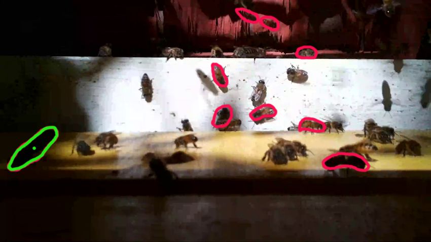
Appl. Sci. 2020, 10, 2042                                                                             2 of 31

three to four years. A prolific queen may lay up to 3000 eggs per day [1]. The drones are male bees.
They have no sting and no means of gathering nectar, secreting wax, or bringing water. Their sole
role is to mate with queens on their bridal trip and instantly die in the act of copulation. Only one
in a thousand gets a chance to mate [1]. All day-to-day colony work is done by the female worker
bees. When workers emerge from their cells, they start cleaning cells in the brood nest. After a week,
they feed and nurse larvae. The nursing assignment lasts one or two weeks and is followed by other
duties such as cell construction, receiving nectar from foragers, and guarding the hive’s entrance.
In their third or fourth week, the female bees become foragers. There are three kinds of foragers: nectar
foragers, pollen foragers, and water foragers. Page [3] argued that pollen foraging is a function of
the number of cells without pollen encountered on the boundary cells and the pollen cells. Thus, if a
forager encounters more empty pollen cells than some value representative of her response threshold,
she leaves the hive for another pollen load. If, on the other hand, she encounters fewer empty cells,
she stops foraging for pollen and engages in nectar or water foraging. The foragers live 5–6 weeks and
do not perform their previous duties within the hive.
      The well-being of a honeybee colony in a hive critically depends on robust forager traffic. Repeated
discrepancies or disruptions in forager traffic indicate that the hive may not be healthy. Thus, accurate
measurement of honeybee traffic in the vicinity of the hive is fundamental for electronic beehive
monitoring (EBM) systems that continuously monitor honeybee colonies to detect and report deviations
from the norm. Our EBM research (e.g., [4–6]), during which we watched hundreds of field-captured
honeybee traffic videos of three different bee races (Carniolan, Italian, and Buckfast), leads us to the
conclusion that honeybee traffic in the vicinity of a Langstroth hive [7] can be divided into three distinct
classes: incoming, outgoing, and lateral. Incoming traffic consists of bees entering the hive either through
the landing pad or holes drilled in supers. Outgoing traffic consists of bees leaving the hive either
from the landing pad or from holes drilled in supers. Lateral traffic consists of bees flying more or
less in parallel to the front side of the hive (i.e., the side with the landing pad). We refer to these three
types of traffic as directional traffic and juxtapose it with omnidirectional traffic [6] where bee motions
are detected regardless of direction.
      In this investigation, we contribute to the body of research on insect and animal flight by
presenting a bee motion estimation algorithm based on digital particle image velocimetry (DPIV) [8]
to measure levels of directional honeybee traffic in the vicinity of a Langstroth hive. The algorithm
does not compute honeybee flight paths or trajectories, which, as our longitudinal field deployment
convinced us [4,6], is feasible only at very low levels of honeybee traffic. Rather, the proposed method
uses DPIV to compute motion vectors, analytically classifies them as incoming, outgoing, or lateral,
and uses the classified vector counts to measure directional honeybee traffic.
      The remainder of our article is organized as follows. In Section 2, we present related work and
connect this investigation to our previous research. In Section 3, we briefly describe the hardware we
built and deployed on Langstroth hives to capture bee traffic videos for this investigation and give a
detailed description of our algorithm to measure directional bee traffic. In Section 4, we present the
experiments we designed to evaluate the proposed algorithm. In Section 5, we give our conclusions.

2. Related Work
      Flying insects and animals, as they move through the air, leave behind air motions which,
if accurately captured, can characterize insect and animal flight patterns. The discovery of digital
particle image velocimetry (DPIV) [8,9] enabled scientists and engineers to start investigating insect
and animal flight topologies. Reliable quantitative descriptions of such flight topologies not only
improve our understanding of how insects and animals fly and capture their flight patterns but may,
in time, result in better designs of micro-air vehicles. For example, Spedding et al. [10] performed a
series of experiments with DPIV to measure turbulence levels in a low turbulence wind tunnel and
argued that DPIV can, in principle, be tuned to measure the aerodynamic performance of small-scale
flying devices.
Appl. Sci. 2020, 10, 2042                                                                          3 of 31

      Several researchers and research groups have used DPIV to investigate various aspects of animal
and insect flight. Henningsson et al. [11] used DPIV to investigate the vortex wake and flight kinematics
of a swift in cruising flight in a wind tunnel. The researchers recorded the swift’s wingbeat kinematics
by a high-speed camera and used DPIV to visualize the birds’ wake. Hedenström et al. [12] showed
that the wakes of a small bat species are different from the wakes of birds by using DPIV to visualize
and analyze wake images. The researchers discovered that in the investigated bat species each wing
generated its own vortex loop and the circulation on the outer wing and the arm wing differed in sign
during the upstroke, which resulted in negative lift on the hand wing and positive lift on the arm wing.
      Spedding et al. [13] used DPIV to formulate a simple model to explain the correct, measured
balance of forces in the downstroke- and upstroke-generated wake over the entire range of flight speeds
in thrush nightingales. The researchers demonstrated the feasibility of tracking the momentum in the
wake of a flying animal. DPIV measurements were used to quantify and sum disparate vortices and to
find that the momentum is not entirely contained within the coarse vortex wake. Muijres et al. [14]
used DPIV to demonstrate that a small nectar-feeding bat increases lift by as much as 40% using
attached leading-edge vortices during slow forward flight. The researchers also showed that the
use of unsteady aerodynamic mechanisms in flapping flight is not limited to insects but is also used
by larger and heavier animals. Hubel et al. [15] investigated the kinematics and wake structure of
lesser dog-faced fruit bats (Cynopterus brachyotis) flying in a wind tunnel. The flow structure in the
spanwise plane perpendicular to the flow stream was visualized using time-resolved PIV. The flight of
four bats was investigated to reveal patterns in kinematics and wake structure typical for lower and
higher speeds.
      Dickinson et al. [16] were the first to use DPIV to investigate insect flight. The researchers used
DPIV to measure fluid velocities of a fruit fly and determine the contribution of the leading-edge vortex
to overall force production. Bomphrey et al. [17] did the first DPIV analysis of the flow field around
the wings of the tobacco hawkmoth (Manduca sexta) in a wind tunnel. During the late downstroke of
Manduca, the flow was experimentally shown to separate at, or near, the leading edge of the wing.
Flow separation was associated with a saddle between the wing bases on the surface of the hawkmoth’s
thorax. Michelsen [18] used DPIV to examine and analyze sound and air flows generated by dancing
honeybees. DPIV was used to map the air flows around wagging bees. It was discovered that the
movement of the bee body is followed by a thin (1–2 mm) boundary layer and other air flows lag
behind the body motion and are insufficient to fill the volume left by the body or remove the air from
the space occupied by the bee body. The DPIV analysis showed that flows collide and lead to the
formation of short-lived eddies.
      Several electronic beehive monitoring projects are related to our research. Rodriguez et al. [19]
proposed a system for pose detection and tracking of multiple insects and animals, which they used
to monitor the traffic of honeybees and mice. The system uses a deep neural network to detect and
associate detected body parts into whole insects or animals. The network predicts a set of 2D confidence
maps of present body parts and a set of vectors of part affinity fields that encode associations detected
among the parts. Greedy inference is subsequently used to select the most likely predictions for the
parts and compiles the parts into larger insects or animals. The system uses trajectory tracking to
distinguish entering and leaving bees, which works reliably under smaller bee traffic levels. The dataset
used by the researchers to evaluate their system consists of 100 fully annotated frames, where each
frame contains 6–14 honeybees. Since the dataset does not appear to be public, the experimental results
cannot be independently replicated.
Appl. Sci. 2020, 10, 2042                                                                           4 of 31

      Babic et al. [20] proposed a system for pollen bearing honeybee detection in surveillance videos
obtained at the entrance of a hive. The system’s hardware includes a specially designed wooden
box with a raspberry pi camera module inside. The box is mounted on the front side of a standard
hive above the hive entrance. There is a glass plate placed on the bottom side of the box, 2 cm above
the flight board, which forces the bees entering or leaving the hive to crawl a distance of ≈11 cm.
Consequently, the bees in the field of view of the camera cannot fly. The training dataset contains
50 images of pollen bearing honeybees and 50 images of honeybees without pollen. The test dataset
consists of 354 honeybee images. Since neither dataset appears to be public, the experimental results
cannot be independently replicated.
      The DPIV-based bee motion estimation algorithm presented in this article improves our previously
proposed two-tier method of bee motion counting based on motion detection and motion region
classification [6] in three respects: (1) it can be used to measure not only omnidirectional but also
directional honeybee traffic; (2) it does not require extensive training of motion region classifiers
(e.g., deep neural networks); and (3) it provides insect-independent motion measurement in that it
does not require training insect-specific recognition models. Our evaluation results are based on four
30-s videos captured by deployed BeePi monitors. Each video consists of 744 frames. Each frame
is manually labeled by a human observer for the number of full bee motions. Thus, the evaluation
dataset for this investigation consists of 2976 manually labeled video frames. To ensure the replicability
of our findings, we have made the videos and frame-by-frame bee motion counts publicly available
(see the Supplementary Materials).

3. Materials and Methods

3.1. Hardware and Data Acquisition
     The video data for this investigation were captured by BeePi monitors, multi-sensor EBM systems
we designed and built in 2014 [4], and have been iteratively modifying [6,21] since then. Each BeePi
monitor consists of a raspberry pi 3 model B v1.2 computer, a pi T-Cobbler, a breadboard, a waterproof
DS18B20 temperature sensor, a pi v2 8-megapixel camera board, a v2.1 ChronoDot clock, and a Neewer
3.5 mm mini lapel microphone placed above the landing pad. All hardware components fit in a single
Langstroth super. BeePi units are powered either from the grid or rechargeable batteries.
     BeePi monitors thus far have had six field deployments. The first deployment was in Logan, UT
(September 2014) when a single BeePi monitor was placed into an empty hive and ran on solar power
for two weeks. The second deployment was in Garland, UT (December 2014–January 2015), when
a BeePi monitor was placed in a hive with overwintering honeybees and successfully operated for
nine out of the fourteen days of deployment on solar power to capture ≈200 MB of data. The third
deployment was in North Logan, UT (April 2016–November 2016) where four BeePi monitors were
placed into four beehives at two small apiaries and captured ≈20 GB of data. The fourth deployment
was in Logan and North Logan, UT (April 2017–September 2017), when four BeePi units were placed
into four beehives at two small apiaries to collect ≈220 GB of audio, video, and temperature data.
The fifth deployment started in April 2018, when four BeePi monitors were placed into four beehives
at an apiary in Logan, UT. In September 2018, we decided to keep the monitors deployed through the
winter to stress test the equipment in the harsh weather conditions of northern Utah. By May 2019, we
had collected over 400 GB of video, audio, and temperature data. The sixth field deployment started
in May 2019 with four freshly installed bee packages and is ongoing with ≈150 GB of data collected
so far.

3.2. Directional Bee Traffic
    The main logical steps of the proposed algorithm are given in Figure 1. Let Ft and Ft+1 be two
consecutive image frames in a video such that Ft is taken at time t and Ft+1 at time t + 1. Let I A1 be a
D × D window, referred to as interrogation area in the PIV literature, selected from Ft and centered at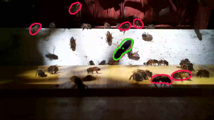
Appl. Sci. 2020, 10, 2042                                                                                       5 of 31

position (i, j). Another D 0 × D 0 window, I A2 , is selected in Ft+1 so that D ≤ D 0 . The position of I A2 in
Ft+1 is the function of the position of I A1 in Ft in that it changes relative to I A1 to find the maximum
correlation peak. In other words, for each possible position of I A1 in Ft , a corresponding position
I A2 is computed in Ft+1 . For example, I A2 in Ft+1 can be centered at the same position (i, j) as I A1
in Ft . The 2D matrix correlation is computed between I A1 and I A2 with the correlation formula in
Equation (1).

                                                D −1 D −1
                                     C (r, s) = ∑       ∑ I A1 (i, j) I A2 (i + r, j + s),
                                                 i =0 j =0                                                         (1)
                                                               0                     0
                                       where r, s ∈   [−b D+ D2 −1 c, . . . , b D+ D2 −1 c]
     In Equation (1), I A1 (i, j) and I A2 (i + r, j + s) are the pixel intensities at location (i, j) in Ft and
(i + r, j + s) in Ft+1 , respectively (see Figure 2). For each possible position (r, s) of I A1 inside I A2 ,
the correlation value C (r, s) is computed. If the size of I A1 is M × N and the size of I A2 is P × Q, then
the size of the C matrix is ( M + P − 1) × ( N + Q − 1). The C matrix records the correlation coefficient
for each possible alignment of I A1 with I A2 . Let C (rm , sm ) be the maximum value in C. If (ic , jc ) is
the center of I A1 , then the positions of (ic , jc ) and (rm , sm ) define a displacement vector ~vic ,jc ,rm ,sm from
location (ic , jc ) in Ft to (ic + rm , jc + sm ) in Ft+1 . This vector is a representation of how the particles
may have moved from Ft to Ft+1 . All displacement vectors form a vector field that can be used to
estimate possible flow patterns. Figure 2 shows the steps of how the cross correlation coefficients are
computed. A faster way to calculate correlation coefficients between two image frames is to use the
Fast Fourier Transform (FFT) and its inverse, as shown in Equation (2). The reason the equation tends
to be computationally faster is that I A1 and I A2 must be of the same size.

                                    C (r, s) =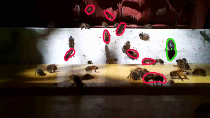
Appl. Sci. 2020, 10, 2042                                                                                          6 of 31

      Figure 2. 2D Correlation Algorithm. The upper image with particles on the left is Ft . The lower image
      on the left is Ft+1 . The region with the light orange borders in the upper image is I A1 . The region with
      the pink borders in the lower image is I A2 . The 3D plot on the right plots all 2D correlation values.
      The highest peak helps to estimate the general flow direction.

       Figure 3 gives the directional vectors computed by the proposed algorithm from two consecutive
640 × 480 video frames with an interrogation window size of 90 and an overlap of 60%. Figure 3a,b
presents two consecutive frames from a 30-s video captured by a deployed BeePi monitor. In Figure 3a,
a single moving bee is indicated by a green rectangle. In Figure 3b, the same bee, again indicated by a
green rectangle, has moved toward the white landing pad (the white strip in the middle of the image)
of the hive. This movement of the bee is reflected in a vector field of eleven vectors shown in Figure 3e.
Figure 3c,d presents two consecutive frames from a different 30-s video captured by the same deployed
BeePi monitor. In Figure 3c, two moving bees are detected: the first bee is denoted by the upper green
rectangle and the second one is denoted by the lower green rectangle. In Figure 3d, the first (i.e., upper)
bee has moved toward the landing pad, while the second (i.e., lower) bee has moved laterally, i.e.,
more or less parallel to the landing pad. The two bee moves are shown in two vector fields in Figure 3f.
The upper vector field that captures the motion of the upper bee contains nine vectors, while the lower
vector field that captures the motion of the lower bee contains only one vector.
       Once the vector fields are computed for a pair of consecutive frames, the directions of these
vectors are used to estimate directional bee traffic levels. Specifically, each vector is classified as lateral,
incoming, or outgoing according to the value ranges in Figure 4. A vector ~v is classified as outgoing if
its direction is in the range [11◦ , 170◦ ], as incoming if its direction is in the range [−11◦ , −170◦ ], and as
lateral if its direction is in the ranges [−10◦ , 10◦ ], [171◦ , 180◦ ], or [−171◦ , −180◦ ].
       Let Ft and Ft+1 be two consecutive frames from a video V. Let I f ( Ft , Ft+1 ), O f ( Ft , Ft+1 ), and
L f ( Ft , Ft+1 ) be the counts of incoming, outgoing, and lateral vectors. For each pair of consecutive
images Ft and Ft+1 , the algorithm computes three non-negative integers: I f ( Ft , Ft+1 ), O f ( Ft , Ft+1 ), and
L f ( Ft , Ft+1 ). If a video V is a sequence of n frames ( F1 , F2 , . . . , Fn ), then we can use I f , O f , and L f to
define the functions Iv (V ), Ov (V ), and Lv (V ) that return the counts of incoming, outgoing, and lateral
vector counts for V, as shown in Equation (3).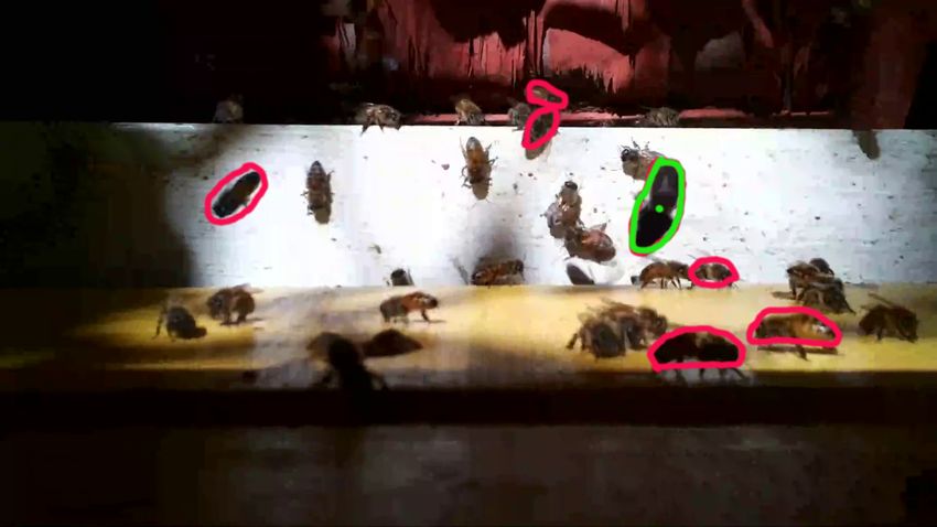
Appl. Sci. 2020, 10, 2042                                                                                                    7 of 31

                                                               n −1
                                                   Iv (V ) =    ∑     I f ( Fi , Fi+1 )
                                                               i =1
                                                               n −1
                                                 Ov ( V ) =     ∑ O f ( Fi , Fi+1 )                                              (3)
                                                               i =1
                                                               n −1
                                                  L v (V ) =    ∑ L f ( Fi , Fi+1 )
                                                               i =1

        For example, let V = ( F1 , F2 , F3 ) such that I f ( F1 , F2 ) = 10, O f ( F1 , F2 ) = 4, L f ( F1 , F2 ) = 3 and
I f ( F2 , F3 ) = 2, O f ( F2 , F3 ) = 7, L f ( F2 , F3 ) = 5. Then, Iv (V ) = I f ( F1 , F2 ) + I f ( F2 , F3 ) = 10 + 2 = 12,
Ov (V ) = O f ( F1 , F2 ) + O f ( F2 , F3 ) = 4 + 7 = 11, and Lv (V ) = L f ( F1 , F2 ) + L f ( F2 , F3 ) = 3 + 5 = 8.
For each pair of consecutive frames Ft and Ft+1 , the omnidirectional motion vector count is defined
as the sum of the values of I f , and O f , and L f , as shown in Equation (4). Then, for each video V,
the omnidirectional vector count Tv (V ) for the video is the sum of the three directional counts, as also
shown in Equation (4).

                             T f ( Ft , Ft+1 ) = I f ( Ft , Ft+1 ) + O f ( Ft , Ft+1 ) + L f ( Ft , Ft+1 )
                                                                                                                                 (4)
                                    Tv (V ) = Iv (V ) + Ov (V ) + Lv (V )

      (a) Image 1                        (b) Image 2                             (c) Image 3                       (d) Image 4

                (e) Vectors from images 1 and 2                                           (f) Vectors from images 3 and 4

      Figure 3. (a,b) Two consecutive frames selected from a 30-s video. (c,d) Two consecutive frames
      selected from a different 30-s video. The vector field in (e) is generated from the images in (a,b);
      the vector field in (f) is generated from the images in (c,d).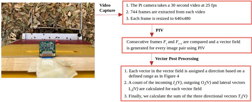
Appl. Sci. 2020, 10, 2042                                                                                  8 of 31

             Figure 4. Degree ranges used to classify DPIV vectors as lateral, incoming, and outgoing.

     Table 1 gives the list of the DPIV parameters we used to run our experiments described in the
next section. In all experiments, only a single pass of DPIV was executed.

                  Table 1. DPIV parameters used in the proposed bee motion estimation algorithm.

                            Parameter                                   Value
                            Img. Size                     160 × 120, 320 × 240, 640 × 480
                      Inter. Win. Size              n × n, where n ∈ {6, 8, 12, 16, 20, 32, 64, 90}
                 Inter. Win. Overlap (%)                              10, 30, 50
                 Inter. Win. Correlation                                 FFT
                Time Delta (DT = 1/FPS)                     0.04 (25 frames per second)
                  Signal to Noise Ratio                peak1/peak2 with a threshold of 0.05
             Spurious Vector Replacement     local mean with kernel size of 2 and max. iter. limit of 15

4. Experiments

4.1. Omnidirectional Bee Traffic
      In our first experiment, we compared the performance of the proposed DPIV-based bee
motion estimation algorithm with our previously proposed two-tier method of omnidirectional
bee motion counting based on motion detection and motion region classification to estimate
levels of omnidirectional bee traffic [6]. In that earlier investigation, we also made a preliminary,
proof-of-concept evaluation of the two-tier method’s performance on four randomly selected bee
traffic videos. Specifically, we took approximately 3500 timestamped 30-s bee traffic videos captured
by two deployed BeePi monitors in June and July 2018. From this collection, we took a random
sample of 30 videos from the early morning (06:00–08:00), a random sample of 30 videos from the early
afternoon (13:00–15:00), a random sample of 30 videos from the late afternoon (16:00–18:00), and a
random sample of 30 videos from the evening (19:00–21:00). Each video consisted of 744 640 × 480
frames. Then, we randomly selected one video from the 30 early morning videos, one from the 30
early afternoon videos, one from the 30 late afternoon videos, and one from the 30 evening videos. We
chose these time periods to ensure that we had videos with different traffic levels.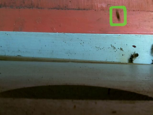
Appl. Sci. 2020, 10, 2042                                                                                9 of 31

     For each of the four videos, we manually counted full bee motions, frame by frame, in each
video. The number of bee motions in the first frame of each video (Frame 1) was taken to be 0. In each
subsequent frame, we counted the number of full bees that made any motion when compared to
their positions in the previous frame. In addition to counting motions of bees present in each pair
of consecutive frames Ft and Ft+1 , we also counted as full bee motions when bees appeared in the
subsequent frame Ft+1 but were not present in the previous frame Ft (e.g., when a bee flew into the
camera’s field of view when Ft+1 was captured).
     We classified the four videos on the basis of our bee motion counts as no traffic (NT) (NT_Vid.mp4),
low traffic (LT) (LT_Vid.mp4), medium traffic (MT) (MT_Vid.mp4), and high traffic (HT) (HT_Vid.mp4).
It took us approximately 2 h to count bee motions in NT_Vid.mp4, 4 h in LT_Vid.mp4, 5.5 h in
MT_Vid.mp4, and 6.5 h in HT_Vid.mp4, for a total of ≈18 h for all four videos. Table 2 is reproduced
from our article [6], where we compared the performance of our four best configurations of the two-tier
method for omnidirectional bee counting: MOG2/VGG16, MOG2/ResNet32, MOG2/ConvNetGS3,
and MOG2/ConvNetGS4. The first element in each configuration (e.g., MOG2 [22]) specifies a motion
detection algorithm; the second element (e.g., VGG16 [23]) specifies a classifier that classifies each
motion region detected by the algorithm specified in the first element.
     We compared the omnidirectional bee motion counts in Table 2 with the omnidirectional bee
motion estimates returned by the DPIV-based bee motion estimation algorithm (i.e., Tv values
in Equation (4)). Since the configuration MOG2/VGG16 gave us the overall best results in our
previous investigation [6], we compared the proposed algorithm’s estimates with the outputs of this
configuration (see the VGG16 column in Table 2). The video frame size was 640 × 480, the interrogation
window size was 90, and the interrogation window overlap was 60%. Let C1 , C2 , and C3 be the
counts returned by the proposed DPIV-based algorithm, the MOG2/VGG16 algorithm, and the human
counter, respectively. Of course, these counts cannot be directly compared, because the former are
motion vector counts while the two latter are actual bee motion counts. Several motion vectors returned
by the proposed algorithm may correspond to a single bee motion. To make a meaningful comparison,
we standardized these three variables to be on the same scale by calculating the mean µ and the
standard deviation σ for each variable, subtracting each observed value v from µ, and dividing by σ.
Thus, the three standardized variables (i.e., C1∗ , C2∗ , and C3∗ ) had an approximate µ of 0 and a σ of 1.
Figure 5 gives the plots of the three standardized variables, C1∗ , C2∗ , and C3∗ , for each of the four videos.

      Table 2. Performance of the system on the four evaluation videos: the columns VGG16, ResNet32,
      ConvNetGS3, and ConvNetGS4 give the bee motion counts returned by the configurations
      MOG2/VGG16, MOG2/ResNet32, MOG2/ConvNetGS3, and MOG2/ConvNetGS4, respectively;
      and the last column gives the human bee motion counts for each video.

        Video          Num. Frames   VGG16     ResNet32     ConvNetGS3      ConvNetGS4       Human Count
    NT_Vid.mp4              742       151          75           182              127                73
    LT_Vid.mp4              744        47          25            57               43               353
    MT_Vid.mp4              743       1245        145           597              316              2924
    HT_Vid.mp4              744      16,647      13,362        16,569           15,109            5738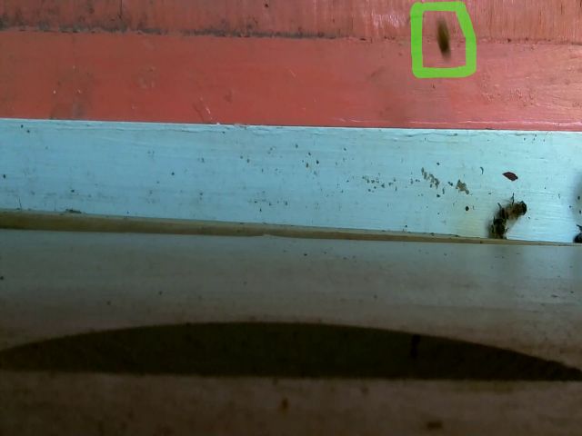
Appl. Sci. 2020, 10, 2042                                                                                        10 of 31

     The plots in Figure 5 of the three standardized variables C1∗ , C2∗ , and C3∗ can be construed as time
series and compared as such. A classical approach for calculating similarity between two time series
is by using Dynamic Time Warping (DTW) (e.g., [24,25]). DTW is a numerical similarity measure
of how two time series can be optimally aligned (i.e., warped) in such a way that the accumulated
alignment cost is minimized. DTW is based on dynamic programming in that the method finds all
possible alignment paths and selects a path with a minimum cost.

                            D (i, j) = di,j + min{ D (i − 1, j − 1), D (i − 1, j), D (i, j − 1)}                      (5)

                      (a) HT_Vid.mp4                                            (b) MT_Vid.mp4

                       (c) LT_Vid.mp4                                           (d) NT_Vid.mp4

      Figure 5. Plots of the three standardized variables on four evaluation videos, no traffic (NT_Vid.mp4),
      low traffic (LT_Vid.mp4), medium traffic (MT_Vid.mp4), and high traffic (HT_Vid.mp4). The total
      number of frames examined were 216,956 video frames. The x-axis is the time (in seconds) when
      each video frame is captured. The y-axis is the values of the standardized variables C1∗ (DPIV), C2∗
      (MOG2/VGG16), and C3∗ (Human Count). C3∗ is the ground truth. Let Ft and Ft+1 be two consecutive
      frames captured at times t and t + 1, 1 ≤ t ≤ 29. C1∗ (t + 1) is the standardized value of T f ( Ft , Ft+1 ),
      C2∗ (t) is the standardized value of the count returned by the MOG2/VGG16 algorithm for Ft , and C3∗ is
      the standardized value of the count returned by the human counter for Ft . C1∗ (1) = C2∗ (1) = C3∗ (1) = 0.
Appl. Sci. 2020, 10, 2042 11 of 31
Let X and Y be two time series such that X = ( x1 , x2 , . . . , xi , . . . , xn ) and Y =
(y1 , y2 , . . . , y j , . . . , ym ), for some integers n and m. An n × m distance matrix D is created where
each cell D (i, j) is the cumulative cost of aligning ( x1 , . . . , xi ) with (y1 , . . . , y j ) defined in Equation (5),
where d(i, j) = d( xi , y j ) = ( xi − y j )2 is the local distance (e.g., Euclidean) between the points xi and y j
from X and Y, respectively. An optimal path is a path with a minimal cumulative cost of aligning
the time series from D (1, 1) to D (n, m). DTW ( X, Y ) is the sum of the pointwise distances along the
optimal path.
Table 3 gives the DTW comparisons of C1∗ (DPIV) and C2∗ (MOG2/VGG16) with the ground
truth of C3∗ (Human Count) for each of the four videos. The DTW coefficients between C1∗ and
C2∗ are lower than the DTW coefficients between C2∗ and C3∗ on all videos except for the no traffic
video NT_Vid.mp4. A closer look at the no traffic video revealed that when the video was taken a
neighboring beehive was being inspected and one of the inspectors slightly pushed the monitored
beehive, which caused the camera to shake. This push resulted in several frames in the video where the
DPIV-based bee motion estimation algorithm detected motions. Overall, in terms of omnidirectional
bee motion counts, the proposed algorithm approximates the human ground truth on par with the
MOG2/VGG16 algorithm. Tables A1–A3 in Appendix A give the DTW similarity scores of the
omnidirectional traffic curves of DPIV with MOG2/ConvGS3, MOG2/ConvGS4, MOG2/ResNet32,
and the human ground truth that show similar results. These results indicate that the proposed
algorithm estimates omnidirectional traffic levels on par with our previously proposed two-tier
algorithm to count omnidirectional bee motions in videos [6].
Table 3. Omnidirectional traffic curve comparison: C1∗ is DPIV; C2∗ is MOG2/VGG16; and C3∗ is Human
Count (ground truth).
DTW vs. Video HT_Vid.mp4 MT_Vid.mp4 LT_Vid.mp4 NT_Vid.mp4
DTW (C1∗ , C3∗ ) 20.75 21.71 15.36 10.53
DTW (C2∗ , C3∗ ) 22.02 22.19 18.13 6.47
4.2. Subpixel Accuracy
We investigated the appropriateness of the traditional 3-point Gaussian sub-pixel accuracy in the
context of estimating bee motions to determine whether the correlation matrices generated Gaussian
curves. We randomly selected several consecutive image pairs from our dataset. For each selected
image pair, the image size was 160 × 120 and the interrogation window size was 12 with a 50% overlap.
To simplify visualization, we selected only the image pairs with a singly bee moving. Figure 6 shows
a sample image pair with the moving bee selected by the green box and the corresponding vectors
generated by DPIV.
We computed the correlation matrices for all motion vectors and visualized them with 3D plots,
as shown in Figure 7. Each 3D plot in Figure 7 corresponds to a vector in the vector map of Figure 6.
Specifically, the first 3D plot in the first row (Figure 7a) corresponds to the first (left) vector in the first
row of the vector map in Figure 6c; the second 3D plot in the first row (Figure 7b) corresponds to the
second (right) vector in the first row of the vector map in Figure 6c; the first 3D plot in the second row
(Figure 7c) corresponds to the first vector in the the second row of Figure 6c; the second 3D plot in
the second row (Figure 7d) corresponds to the second vector in the second row of the vector map in
Figure 6c; the first 3D plot in the third row (Figure 7e) corresponds to the first vector in the third row
of the vector map in Figure 6c; and the second 3D plot in the third row (Figure 7f) corresponds to the
second vector in the third row of the vector map in Figure 6c. Since the vectors in the first row are
small, we scaled the plots to better visualize the corresponding distribution (see Figure 8). Another
sample image pair with the corresponding DPIV vectors and plots are given in Figures A1 and A2 in
Appendix A.Appl. Sci. 2020, 10, 2042 12 of 31
By analyzing such 3D plots of correlation vectors of two consecutive images with single bees
moving, we concluded that all correlation maps follow Gaussian distribution. We also observed that
not all plots have distinct peaks. For example, the first plot in the second row in Figure 7 has a distinct
peak while the first plot of the third row has no distinct peaks. Therefore, the traditional three-point
Gaussian sub-pixel accuracy method can be used to determine better peaks in such cases. Another
observation we made is that the middle vectors tend to have larger magnitudes than the vectors in the
higher and lower rows. This observation seems to indicate that the body of the bee, as a whole, causes
maximum motion and, as a consequence, it is reasonable to treat whole bees as tracers. The bee body
parts such as wings, thorax, and legs result in smaller motions or are not detected at all.
(a) Frame 1 (b) Frame 2
(c) DPIV motion vectors
Figure 6. Two consecutive video frames, Frame 1 and Frame 2 with a single moving bee and corresponding
DPIV motion vectors.Appl. Sci. 2020, 10, 2042 13 of 31
(a) Correlation map for Vector 1 (b) Correlation map for Vector 2
(c) Correlation map for Vector 3 (d) Correlation map for Vector 4
(e) Correlation map for Vector 5 (f) Correlation map for Vector 6
Figure 7. 3D plots of correlation matrices for the motion vectors in Figure 6c. Each row in the figure
corresponds to each row in the vector plot of Figure 6c.Appl. Sci. 2020, 10, 2042 14 of 31
(a) Scaled correlation map for Vector 1 (b) Scaled correlation map for Vector 2
Figure 8. Scaled 3D map for the correlation matrices of Figure 7a,b respectively.
4.3. Interrogation Window Sizes
We used a single bee as a tracer. However, a single bee motion generates multiple motion
vectors, because multiple bee parts (wings, thorax, legs, etc.) are moving simultaneously, which
may be captured in interrogation windows. We executed additional experiments with our algorithm
to evaluate its performance with different image and interrogation window sizes. Specifically, we
experimented with three image sizes: 160 × 120, 320 × 240, and 640 × 480. For each image size, we
manually calculated the bee size in pixels. For 160 × 120 images, the average bee size was equal to
8 × 8 pixels; for 320 × 240 images, the average bee size was equal to 16 × 16; and for images 640 × 480,
the average bee size was equal to 32 × 32. For each image size and bee size, we tested different sizes of
interrogation windows (i.e., smaller than the bee size, equal to the bee size, and larger than the bee
size) with different amounts of interrogation window overlap. We made no attempt to improve the
quality of the data or reduce the uncertainty of particle displacement, because the system should work
out-of-the-box in the field on inexpensive, off-the-shelf hardware for beekeepers and apiary scientists
worldwide to afford it.
To remove the spurious vectors, we calculated the signal to noise (SNR) ratio for each generated
correlation matrix. The SNR was calculated by finding the highest peak (p1 ) and the second highest
peak (p2 ) in the correlation matrix and then computing SNR as their ratio (i.e., SNR = p1 /p2 ).
If the SNR values were less than a given threshold (0.05 in our case), the corresponding vectors
were considered spurious and removed. Such vectors were replaced by the weighted average of the
neighboring vectors. We used a kernel size (K) of 2 and a local mean to assign the weights with the
formula 1/((2K + 1)2 − 1). We used a maximum iteration limit of 15 and a tolerance of 0.001 to replace
the spurious vectors.
Table 4 gives the results of our experiments with different interrogation window sizes on 640 × 480
image frames in the high-traffic video HT_Vid.mp4. The last two columns give the dynamic time
warping (DTW) results. Tables for the other image sizes and videos (Tables A5–A15) are given in
the Appendix A. As these tables show, the best similarity with the ground truth was achieved when
the interrogation window was twice the size of the bee or higher for all three image sizes and an
interrogation window overlap of 30% or higher.Appl. Sci. 2020, 10, 2042 15 of 31
Table 4. DTW values for HT_Vid.mp4 with image size of 640 × 480; C1∗ is DPIV; C2∗ is MOG2/VGG16;
and C3∗ is Human Count (ground truth).
Img. Size Bee Size Inter. Win. Size % Overlap Pix Overlap DTW(C1∗ ,C3∗ ) DTW(C2∗ ,C3∗ )
640 × 480 32 × 32 28 10 13 19.1884 22.02607
28 30 8 18.4507 22.02607
28 50 14 18.6779 22.02607
32 10 3 19.3991 22.02607
32 30 10 19.8832 22.02607
32 50 16 17.7650 22.02607
36 10 4 19.4907 22.02607
36 30 11 17.4369 22.02607
36 50 18 20.0698 22.02607
64 10 6 22.0901 22.02607
64 30 19 21.1846 22.02607
64 50 32 20.1906 22.02607
90 10 9 23.4524 22.02607
90 30 27 20.8363 22.02607
90 50 45 21.3194 22.02607
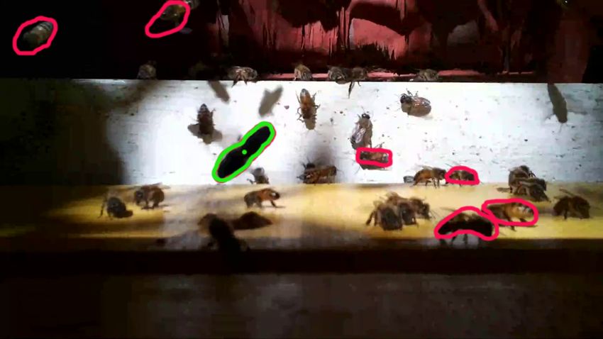
In the course of our investigation, we discovered that in some videos there were bees which
flew very fast. Figure 9 gives the first and last frames (Frames 1 and 7, respectively) in a seven-frame
sequence from a high bee traffic video. Table A3 in the Appendix A gives all the frames in the sequence.
In Figure 9, a fast moving bee is delineated in each frame by a green polygon. The bee is moving right to
left. The coordinates of the green dot (a single pixel) in each polygon are x = 507.0, y = 1782.0 in Frame
1 and x = 660.0, y = 151.5 in Frame 7. The pixel displacements of the green dot for this sequence are as
follows: 220.9 pixels between Frames 1 and 2 (first displacement); 218.5 pixels between Frames 2 and 3
(second displacement); 247.6 pixels between Frames 3 and 4 (third displacement); 329.7 pixels between
Frames 4 and 5 (fourth displacement); 347.6 pixels between Frames 5 and 6 (fifth displacement); and
303.1 pixels between Frames 6 and 7 (sixth displacement). The total pixel displacement of the green dot
between Frames 1 and 7 is ≈1667.4 pixels. The average pixel displacement per frame is ≈277.9 pixels.
The pi camera used in our investigation is not sufficiently powerful to capture all such displacements.
In our system, the maximum pixel displacement per frame is set to 40 pixels, which represents the
maximum velocity that our system can currently handle. As the pi hardware improves, we hope to
raise this parameter to 60 or 80 pixels.
(a) Frame 1 (b) Frame 7
Figure 9. The first and last frames (Frames 1 and 7, respectively) from a sequence of seven consecutive
frames taken from a high bee traffic video; the entire seven-frame sequence is given in Table A3.Appl. Sci. 2020, 10, 2042 16 of 31
4.4. Directional Bee Traffic
The two-tier method of bee motion counting proposed in our previous investigation [6] is
omnidirectional in that it counts bee motions regardless of direction. Therefore, this method cannot be
used to estimate incoming, outgoing, or lateral bee traffic. The algorithm proposed in this article, on
the other hand, can be used to estimate these types of bee traffic.
In another series of experiments, we sought to investigate whether the proposed algorithm can be
used to estimate how closely incoming traffic matches outgoing traffic in healthy beehives. In principle,
in healthy beehives, levels of incoming bee traffic should closely match levels of outgoing bee traffic,
because all foragers that leave the hive should eventually come back. Of course, if the levels of two
traffic types are treated as time series, local mismatches are inevitable, because some foragers that leave
the hive at the same time may not return at the same time because they fly to different foraging sources.
However, the overall matching tendency should be apparent. Departures from this tendency can be
treated as deviations from normalcy and may lead to manual inspection. For example, a large number
of foragers leaving the hive at a given time and never coming back may signal that a swarm event has
taken place. On the other hand, if the level of incoming traffic greatly exceeds the corresponding level
of outgoing traffic over a given time segment, a beehive robbing event may be underway.
To estimate how closely the levels of outgoing and incoming bee traffic match, we took 292 30-s
videos (i.e., all the videos captured by a BeePi monitor deployed on a healthy beehive from 1–5 July
2018 and 8–14 July 2018 (≈24 videos per day)) and computed the values of Iv and Ov (see Equation (3))
for each video with the proposed algorithm. The video frame size was 640 × 480, the interrogation
window size was 90, and the interrogation window overlap was 60%. Figure 10 shows the plots of
the values of Iv and Ov for all videos on four days from the specified period. As can be seen from
these plots, on many days in a healthy beehive the estimated levels of incoming and outgoing traffic
are likely to be very close. Spikes in outgoing curves tend to follow spikes in incoming curves and
vice versa.
We computed the DTW similarity scores between each outgoing bee traffic curve and each
incoming bee traffic curve in Figure 10. Table 5 gives these DTW scores. These scores indicate that the
outgoing and incoming curves tend to match closely on the same day and tend to be dissimilar on
different days. In particular, the DTW scores between the incoming and outgoing bee traffic curves
on the same days, shown in the diagonal, are all below 5. The values are almost twice as high when
the incoming and outgoing curves are from different days. Table A4 in Appendix A gives the DTW
similarity scores for all twelve days in the sampled period. The blue diagonal values in the table
show the DTW similarity scores between the incoming and outgoing traffic curves on the same day.
The statistics for the diagonal values are: median = 4.75, µ = 6.1, and σ = 2.85. The statistics for the
other 132 non-diagonal values (i.e., DTW similarities between traffic curves on different days) are:
median = 13.145, µ = 13.28, σ = 2.99. These statistics suggest possible ranges for monitoring DTW
similarity scores between incoming and outgoing traffic curves for healthy beehives.
On two days in the sample, 3 July 2018 and 5 July 2018, as can be seen in Table A4, the DTW
similarity scores between the outgoing and incoming curves were above 10 on the same day.
Figure 11a,b shows traffic curves for these two days. Our manual analysis of the videos on these two
days revealed that the incoming bees were flying into the beehive too fast for DPIV to detect motion in
the videos captured by a raspberry pi camera, which resulted in the mismatch between the incoming
and outgoing traffic estimates.Appl. Sci. 2020, 10, 2042 17 of 31
(a) 4 July 2018 (b) 8 July 2018
(c) 9 July 2018 (d) 11 July 2018
Figure 10. Plots of Iv and Ov values computed by the proposed algorithm for 4, 8, 9, and 11 July 2018.
Table 5. DTW similarity scores between outgoing and incoming traffic curves in Figure 10.
Outgoing
2018-07-04 2018-07-08 2018-07-09 2018-07-11
Incoming
4 July 2018 4.78 9.58 10.43 11.49
8 July 2018 12.36 4.32 11.42 10.39
9 July 2018 10.90 11.94 4.69 9.59
11 July 2018 14.08 10.18 9.37 4.43
(a) 3 July 2018 (b) 5 July 2018
Figure 11. Plots of Iv and Ov values for 3 July 2018 and 5 July 2018. DTW similarity of the curves on 3
July is 12.436; DTW similarity of the curves on 5 July is 10.179.Appl. Sci. 2020, 10, 2042 18 of 31
4.5. DPIV on Raspberry Pi
DPIV is computationally expensive on the raspberry pi hardware even when cross correlation
is implemented with FFT (see Equation (2)). In implementing our algorithm, we used the OpenPIV
library (http://www.openpiv.net), a community driven initiative to develop free and open-source
particle image velocimetry software. Since in our BeePi monitors all data capture and computation is
done on raspberry pi computers, it is imperative that DPIV run on the raspberry pi hardware.
We tested our algorithm on a single raspberry pi 3 model B v1.2 computer on several 30-s videos
from our dataset. The video frame size was 640 × 480, the interrogation window size was 90, and
the interrogation window overlap was 60%. On average, it took ≈2.5 h for the algorithm to process
a single 30-s video. This result is unacceptable to us, because each BeePi monitor records a 30-s
video every 15 min from 8:00 to 21:00 every day. An obvious solution is cloud computing where
the captured videos are processed in the cloud by a collection of GPUs. We rejected this solution,
because from the beginning of the BeePi project in 2014 we made it a priority to avoid external
dependencies such as continuous Internet and cloud computing. In remote areas, BeePi monitors
should function as self-configurable and self-contained networks that rely exclusively on local area
networking mechanisms (e.g., as an ad hoc network).
Since the raspberry pi 3 model B v1.2 computer has four CPUs, we decided to introduce
multi-threading into our algorithm to reduce video processing time. A BeePi monitor records videos
at ≈25 frames per second. Thus, a 30-s video generates 743–745 frames. Each thread ran on a separate
CPU to process a subset of frames. Specifically, Thread 1 processed Frames 1 processed 185, Thread
2 processed Frames 185–370, Thread 3 processed Frames 370–555, and Thread 4 processed Frames
555–743/745. It should be noted that, to handle boundary frames, there is a one frame overlap between
the ranges because DPIV works on pairs of consecutive frames. Multi-threading reduced the average
video processing time from 2.5 h to 1 h 12 min.
After multi-threading, we introduced parallelism to our system by distributing the algorithm’s
computation over six raspberry pi computers. We chose to experiment with six raspberry pi computers,
because they easily fit into a single deep Langstroth super (i.e., a wooden box) placed on top of a
beehive [26,27]. The current BeePi hardware also fits into a single deep super. In this six-node network,
one node acts as a dispatcher in that it captures video via a raspberry pi camera and dispatches video
frames to the other five nodes that process them and return the results back to the dispatcher. In this
architecture, the dispatcher sends Frames 1–148 to Node 1, Frames 148–296 to Node 2, Frames 296–444
to Node 3, Frames 444–592 to Node 4, and Frames 592–743/745 to Node 5. Each processing node
uses multi-threading, described above, to compute directional vectors, classifies them as incoming,
outgoing, and lateral, and returns these vector counts to the dispatcher. We timed each task in the
system on ten 30-s videos. Table 6 details our measurements. The sum total of the third column is equal
to 1169.462 s ≈ 19.49 min, which is the total time our six-node network takes to process a 30-s video.
Table 6. Average video processing performance of six-node ad hoc network.
Task Executive Time (in sec)
Frame Generation Dispatcher Node 70.826
Frame Dispatch Dispatcher Node 211.116
Frame Processing 5 Processing Nodes 887.52Appl. Sci. 2020, 10, 2042 19 of 31
Through multi-threading and parallelism, we managed to reduce the processing time of a single
video from 2.5 h to below 20 min, which makes it feasible to process all videos captured in one 24-h
period. In the current version of the BeePi monitor, video recording starts at 8:00 and ends at 21:00
(i.e., 13 h or 780 min) and records a 30-s video every 15 min. If there are no hardware disruptions, there
are 52 videos recorded every 24 h. The period from 21:00 of the current day to 8:00 of the next day
(i.e., 11 h or 660 min) is the video recording downtime during which the BeePi monitor does no video
recording and records only temperature and audio every 15 min, neither of which is computationally
taxing. During the video recording period, the monitor spends 2 min per hour (four 30-s videos) on
recording a video for a total of 26 min per day (13-h video capturing period with 2 min of actual video
recording per hour), which makes a total of 754 min (754 = 780 − 26) available for video processing
during the video recording period. During the video recording downtime (660 min), the monitor can
also process videos. Therefore, every 24 h period, 1414 (1414 = 754 + 660) min are available for video
processing. However, to process all 52 videos captured every 24 h, the six-node network requires only
1040 min. Thus, the six-node ad hoc network can process all the videos recorded in the current 24-h
period before the next 24-h data capture period begins.
5. Conclusions
Our experiments indicate that the proposed DPIV-based bee motion estimation algorithm
performs on par with the two-tier bee motion counting algorithm proposed in our previous research [6]
in terms of measuring omnidirectional honeybee traffic. However, unlike the two-tier algorithm
that can estimate only omnidirectional honeybee traffic, the proposed algorithm can measure both
omnidirectional and directional honeybee traffic. The proposed algorithm shows that DPIV can be
used not only for quantifying particle velocities but also for analyzing instantaneous and longitudinal
flow structures.
Another advantage of the current algorithm is that it does not rely on image classification and,
consequently, can be used to measure traffic of other insects such as bumble bees and ants. Insomuch
as DPIV is a purely analytical technique, it requires no machine learning and no large curated datasets.
By contrast, our two-tier algorithm uses machine learning methods (deep neural networks and random
forests) that took us 1292.77 GPU h (53.87 days) to train, test, and validate on our curated datasets of
167,261 honeybee images [6,28–30]. The network of six raspberry pi computers can process all captured
videos within every 24-h data capturing period. The fact that the proposed DPIV-based bee motion
estimation algorithm provides us directionality and insect-independent motion measurement is an
acceptable price to pay for its relative slowness. As the raspberry pi hardware improves, we expect
this processing time to decrease.
A fundamental limitation of DPIV is its dynamic velocity range (DVR) [31], which is the ratio of
the maximum measurable velocity and the minimum measurable velocity. The maximum measurable
velocity is the maximum allowable particle displacement within each interrogation area on the
paired images (see Figure 2). The minimum measurable velocity is the smallest measurable particle
displacement between pixels in the paired images. To overcome the DPIV limitation, traditional
DPIV research has required significant capital and maintenance investments, which confined DPIV
applications mostly to academic or industrial research environments [32]. By distributing the
algorithm’s computation over six raspberry pi computers, we showed that useful DPIV-based results
can be obtained on a hardware base that costs less than 1000 USD. This result bodes well for citizen
science in that the hardware base can be replicated without significant capital and maintenance costs.
We are also currently investigating several techniques of combining multiple neighboring vectors into
a single bee. While our preliminary experiments indicate that such techniques may work on low-traffic
and medium-traffic videos, they may have issues with high-traffic videos.Appl. Sci. 2020, 10, 2042 20 of 31
We have learned from this investigation that obtaining ground truth videos to estimate the
accuracy of bee motion counts is very labor intensive and time consuming. It took us ≈18 h to obtain
human bee motion counts on four videos of live honeybee traffic. We are currently working on curating
more live honeybee traffic videos and hope to make them public in our future publications.
One curious observation we have made about lateral traffic is that the orientation of the bees
engaged in it typically remains perpendicular to the hive (i.e., the bees’ heads face the hive). Another
curious observation we have made about lateral traffic is that sometimes a bee engages in lateral
traffic before entering the hive and sometimes, after doing several sidewise maneuvers, she leaves
the vicinity of the hive captured by the camera. The laterally moving bees that eventually enter the
hive may use lateral moves to better home in on the entry point, whereas the laterally moving bees
that fly away might be stray bees looking for a new home or scouts from other hives checking if the
hive is appropriate for robbing. As computer scientists, however, we have no explanation of these
observations and leave them for entomologists to investigate.
We made no attempt in this investigation to estimate the uncertainty of a DPIV displacement
field. In our future work, we plan to consider applying the methods proposed by Wieneke [33] and
evaluated by Sciacchitano et al. [34] to estimate the uncertainty of generated displacement fields.
However, the application of such methods will have to undergo a detailed cost–benefit analysis in
view of our ultimate objective to obtain reliable and consistent bee traffic measurements from digital
videos on inexpensive hardware that can be replicated by third parties. We are not concerned with
flight trajectories or flow patterns as such. While the latter may turn out to be a significant research
by-product and a contribution, they are not the primary focus of video-based electronic beehive
monitoring. We plan to focus our future work on effective, computationally feasible methods to match
the numbers of bees leaving the hive with the numbers of bees entering the hive and using significant
mismatches as indicators that the hive is not healthy or is under stress. Another possible improvement
that we plan to introduce into our system is the application of fast background elimination techniques
to the video frames prior to DPIV. More uniform backgrounds will enable us to experiment with larger
interrogation windows and multi-pass DPIV to reduce noise and uncertainty.
Our long-term objective has been, and will continue to be, the development of an open design
and open data electronic beehive monitoring (EBM) platform for researchers, practitioners, and citizen
scientists worldwide who want to monitor their beehives or use their beehives as environmental
monitoring stations [35]. Our approach is based on the following four principles. First, the EBM
hardware should be not only open design but also 100% replicable, which we ensure by using
exclusively readily available off-the-shelf hardware components [26,27]. Second, the EBM software
should also be 100% replicable, which we achieve by relying on open source resources. Third,
the project’s hardware should be compatible with standard beehive models used by many beekeepers
worldwide (e.g., the Langstroth beehive [7] or the Dadant beehive [36]) without any required structural
modifications of beehive woodenware. Fourth, the sacredness of the bee space should be preserved in
that the deployment of EBM sensors should not be disruptive to natural beehive cycles.
Supplementary Materials: The following are available online at http://www.mdpi.com/2076-3417/10/6/2042/
s1, The supplementary materials include four CSV files with frame-by-frame full bee motion counts and the
corresponding four honeybee traffic videos. Due to space limitations, we could not include the 292 honeybee
traffic videos we used in our directional honeybee traffic experiments. Interested parties should contact the second
author directly if they want to obtain the videos.
Author Contributions: Supervision, Project Administration, and Resources, V.K.; Conceptualization and
Software, S.M. and V.K.; Data Curation, V.K. and S.M.; Writing—Original Draft Preparation, V.K. and S.M.
Writing—Review and Editing, V.K. and S.M.; Investigation and Analysis, S.M. and V.K.; and Validation, S.M. and
V.K. All authors have read and agreed to the published version of the manuscript.
Funding: This research was funded, in part, by our Kickstarter fundraisers in 2017 [26] and 2019 [27].
Acknowledgments: We would like to thank all our Kickstarter backers and especially our BeePi Angel Backers
(in alphabetical order): Prakhar Amlathe, Ashwani Chahal, Trevor Landeen, Felipe Queiroz, Dinis Quelhas,
Tharun Tej Tammineni, and Tanwir Zaman. We express our gratitude to Gregg Lind, who backed both fundraisers
and donated hardware to the BeePi project. We are grateful to Richard Waggstaff, Craig Huntzinger, and RichardYou can also read