Classification-Aided SAR and AIS Data Fusion for Space-Based Maritime Surveillance - MDPI
←
→
Page content transcription
If your browser does not render page correctly, please read the page content below
remote sensing
Article
Classification-Aided SAR and AIS Data Fusion for Space-Based
Maritime Surveillance
Maximilian Rodger                   and Raffaella Guida *

                                           Surrey Space Centre, University of Surrey, Guildford GU2 7XH, UK; m.rodger@surrey.ac.uk
                                           * Correspondence: r.guida@surrey.ac.uk

                                           Abstract: A wide range of research activities exploit spaceborne Synthetic Aperture Radar (SAR)
                                           and Automatic Identification System (AIS) for applications that contribute to maritime safety and
                                           security. An important requirement of SAR and AIS data fusion is accurate data association (or
                                           correlation), which is the process of linking SAR ship detections and AIS observations considered to
                                           be of a common origin. The data association is particularly difficult in dense shipping environments,
                                           where ships detected in SAR imagery can be wrongly associated with AIS observations. This often
                                           results in an erroneous and/or inaccurate maritime picture. Therefore, a classification-aided data
                                           association technique is proposed which uses a transfer learning method to classify ship types in
                                           SAR imagery. Specifically, a ship classification model is first trained on AIS data and then transferred
                                           to make predictions on SAR ship detections. These predictions are subsequently used in the data
                                           association which uses a rank-ordered assignment technique to provide a robust match between the
                                           data. Two case studies in the UK are used to evaluate the performance of the classification-aided data
                                           association technique based on the types of SAR product used for maritime surveillance: wide-area
                                           and large-scale data association in the English Channel and focused data association in the Solent.
                                           Results show a high level of correspondence between the data that is robust to dense shipping or
                                           high traffic, and the confidence in the data association is improved when using class (i.e., ship type)
                                 information.


Citation: Rodger, M.; Guida, R.            Keywords: synthetic aperture radar (SAR); Sentinel-1; ICEYE-X2; automatic identification system
Classification-Aided SAR and AIS           (AIS); data fusion; data association; ship classification; ship detection; maritime surveillance
Data Fusion for Space-Based
Maritime Surveillance. Remote Sens.
2021, 13, 104. https://doi.org/
10.3390/rs13010104                         1. Introduction
                                                The use of spaceborne Synthetic Aperture Radar (SAR) and Automatic Identification
Received: 17 November 2020
                                           System (AIS) for space-based maritime surveillance has recently seen significant interest
Accepted: 23 December 2020
                                           on an international scale. The primary advantages of SAR include its wide-area coverage
Published: 30 December 2020
                                           and day and night all-weather observation capabilities. In satellite SAR imagery, objects
                                           on the sea surface such as ships and offshore platforms are detected as a collection of
Publisher’s Note: MDPI stays neu-
tral with regard to jurisdictional clai-
                                           bright pixels on a dark background. The AIS is a radio-based communications system that
ms in published maps and institutio-
                                           exchanges information (e.g., the ship’s identity, type, dimensions, position, speed, etc.)
nal affiliations.
                                           between ships and coastal stations [1]. Recently, advancements in AIS technology have also
                                           meant that shipborne AIS signals are now reliably received by satellites in low-Earth orbit
                                           (Satellite-AIS or Sat-AIS), thereby extending its surveillance capability to the open ocean
                                           and beyond the range of terrestrial-based networks. The data fusion of SAR and AIS allows
Copyright: © 2020 by the authors. Li-      the observations from each sensor to be combined to provide an effective understanding of
censee MDPI, Basel, Switzerland.           maritime activities at sea.
This article is an open access article          The data association of SAR and AIS (also called ‘correlation’ or ‘matching’) provides
distributed under the terms and con-
                                           the basis for data fusion. This is the process of linking SAR ship detections and AIS obser-
ditions of the Creative Commons At-
                                           vations considered to be of a common origin. The data association is particularly important
tribution (CC BY) license (https://
                                           for applications and research which use AIS data as a source of ground truth, to both
creativecommons.org/licenses/by/
                                           identify and validate ship detections in SAR imagery. This is demonstrated in various
4.0/).

Remote Sens. 2021, 13, 104. https://doi.org/10.3390/rs13010104                                       https://www.mdpi.com/journal/remotesensing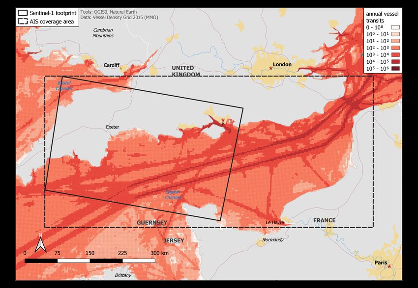
Remote Sens. 2021, 13, 104                                                                                            2 of 26

                             surveillance applications, including maritime monitoring [2–5], piracy activity [6,7], fishing
                             vessel activity [8–11], polluter identification [12–14] and ice navigation [15]. The detection
                             of non-cooperative (or so-called “dark”) ships which have missing AIS information is of
                             particular interest in these applications. This is because ships can be ‘dark’ for a number
                             of reasons. For example, some ships are exempt from transmitting AIS due to their size
                             and class [1]. Conversely, some ships intentionally avoid detection for both illicit and
                             non-illicit reasons such as carrying out illegal fishing [11] or hiding fishing activities from
                             competitors. There are also a wide range of research activities which use SAR and AIS. Two
                             of the most common research areas include the development and validation of SAR ship
                             detection algorithms [16–21] and the evaluation of SAR ship classification models [22–27].
                             This also includes the development of open benchmark datasets intended for these research
                             areas [28–30]. Therefore, a robust and accurate method of data association is essential for
                             the rapidly growing number of applications and research involving SAR and AIS.
                                   In the scientific literature, the data association between SAR and AIS has been predom-
                             inately carried out using simple methods such as Nearest Neighbour (NN) [20,31–35]. The
                             NN is a form of proximity search that assigns data based on a minimum distance, where
                             the ‘distance’ is defined by a selected distance metric or threshold. Optimal methods have
                             been implemented such as Global Nearest Neighbour (GNN) [21,36,37], which requires
                             solving the assignment problem [38,39]. This involves computing the lowest ‘cost’ (i.e., the
                             distance) for all assignments and, unlike the suboptimal NN, determines a unique pairing
                             between observations. Additionally, techniques commonly found in pattern recognition
                             and computer vision have been recommended for SAR and AIS data association based
                             on simulated data [40,41], while being implemented for optical and AIS [42]. The basic
                             principle involves recovering the spatial transformation that aligns the positions of the
                             two sets of observations (or point sets). In a previous publication, it is demonstrated that
                             the performance of all of these techniques depends primarily on the temporal difference
                             (or ‘gap’) between the sensor acquisitions as well as the ship density [43]. In congested
                             areas, ships detected in SAR imagery can be wrongly associated with AIS observations
                             resulting in mis-associations. It is shown that GNN outperforms both NN and techniques
                             that are based exclusively on spatial transformations. Therefore, a modified GNN approach
                             is implemented in this work.
                                   Two other processes are carried out before data association. The first addresses the
                             temporal difference between the two sensor acquisitions and involves interpolating and/or
                             extrapolating the AIS-reported positions to the time of the SAR image acquisition (also
                             called ‘AIS position projection’). In the literature, methods implemented vary from simple
                             linear methods such as dead reckoning [3,15,33,35,40,44] to more involved methods such
                             as spline interpolation [32,34] and knowledge-based interpolation [36]. However, these
                             methods have an upper limit to their performance, where for large temporal differences
                             the uncertainty in the estimated position becomes very large. A technological solution
                             has emerged in new generation spaceborne SAR missions which have the SAR sensor and
                             AIS receiver co-located on the same platform (e.g., NovaSAR-1 [45], PAZ mission [46] and
                             RCM [47]). This allows for nearly contemporaneous data acquisition and alleviates the
                             dependency on interpolation and/or extrapolation methods for large temporal differences.
                             The current trend of growing Sat-AIS and SAR microsatellite constellations also provides a
                             greater chance for data alignment.
                                   The second process deals with the well-known effect observed in SAR imagery that,
                             when an object is moving with a non-zero range velocity component, it will appear dis-
                             placed in the azimuth direction [48,49]. This is known as azimuth image shift (or Doppler
                             shift) and can give rise to the interesting phenomenon where moving ships appear dis-
                             placed from their wake and wave pattern. The formulae for quantifying this displacement
                             (and equally the radial velocity) for satellite SAR imagery are also well-known [2,50,51].
                             In studies using SAR and AIS data, the displacement is typically compensated for by using
                             the AIS-reported velocity in conjunction with the satellite and SAR viewing geometry
                             parameters [31,36,44,52].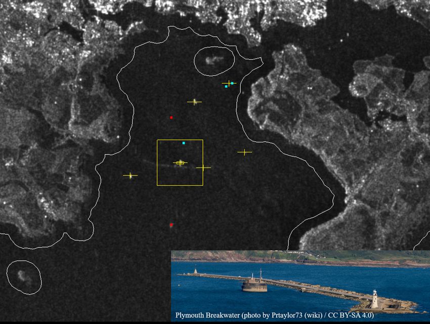
Remote Sens. 2021, 13, 104                                                                                           3 of 26

                                    The purpose of this study is to demonstrate an improved method that achieves a high
                             level of correspondence between the data, especially in dense shipping environments. The
                             method utilises a SAR ship classification model based on AIS transfer learning, which has
                             recently shown to be an effective alternative to conventional SAR ship classification [53,54].
                             The returned class information is subsequently used to maximise the confidence in the data
                             association. The data association between SAR and AIS is formulated as an m-best two-
                             dimensional (2D) assignment problem [39,55], which is solved using the Jonker–Volgenant
                             algorithm [56]. This returns not only the best (optimal) AIS-SAR assignments, but also
                             the second, third, and, in general, the mth best assignments. The advantage of this rank-
                             ordered approach means that a robust match between the data can be achieved, where class
                             and static information (i.e., the ship type and dimensions) is used to reduce the ambiguity
                             in the association. Two case studies in the UK are used to evaluate the performance of the
                             classification-aided data association technique based on the types of SAR product used for
                             maritime surveillance: wide-area and large-scale data association in the English Channel
                             (i.e., larger swath, lower resolution SAR) and focused data association in the Solent (i.e.,
                             smaller swath, higher resolution SAR).

                             2. Materials and Methods
                                  Figure 1 shows a generalised workflow for the method. The fusion workflow is
                             designed to accept input data from various sources as well as SAR imagery products with
                             different imaging modes. The main processes in the workflow include SAR image and
                             AIS data processing, the training of a ship classification model, and data association of
                             the SAR and AIS datasets. The objective of SAR image processing (or ship detection) is to
                             detect objects on the sea surface in the SAR image. The objective of AIS data processing is
                             to prepare AIS data to be matched with the SAR ship detections. The ship classification
                             model uses a transfer learning method to make predictions of the SAR ship detections’
                             ship type. This information is used in the data association which returns a robust match
                             between the SAR (SAR D ) and AIS (AISD ) datasets. These processes are described in more
                             detail in the following subsections.

                                   Figure 1. Fusion workflow for SAR and AIS datasets.

                             2.1. Ship Detection
                                  The Search for Unidentified Maritime Objects (SUMO) software is used for ship
                             detection, which is an open-source ship detection software developed by the European
                             Commission’s Joint Research Centre (JRC) [57]. The SUMO software implements the
                             SUMO algorithm which is based on a Constant False Alarm Rate (CFAR) detector and uses
                             a K-distribution to model the sea clutter [19]. The SUMO processing parameters are given
                             in Table 1. A 250 m seaward-buffered land mask is applied to ensure detection is limited
                             to the sea surface and not over land which can give rise to false alarms. The detection
                             threshold values are slightly raised above the default values (by 0.3 as suggested in [57]) in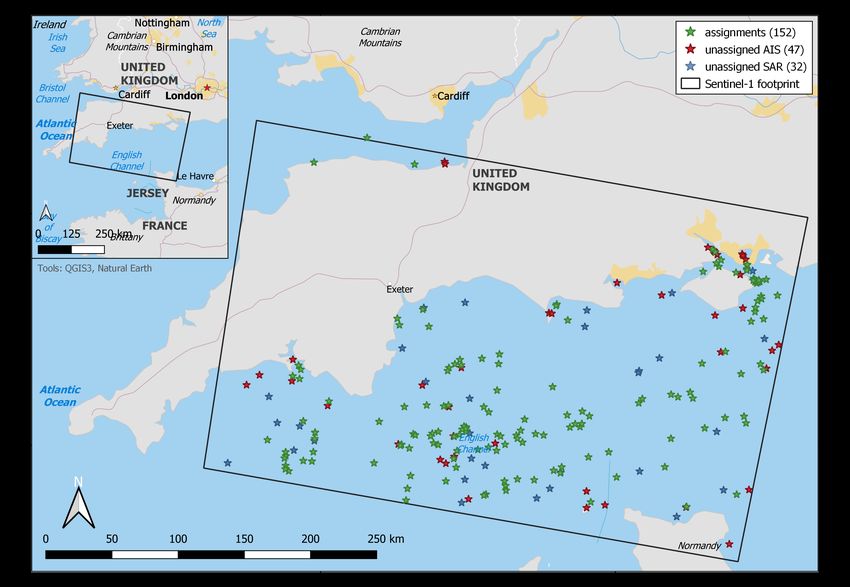
Remote Sens. 2021, 13, 104                                                                                            4 of 26

                             order to limit the number of false alarms. However, this also means very small targets may
                             not be detected by the algorithm.
                                    Discrimination involves removing false alarms. The likelihood of a detection being a
                             false alarm is determined by considering its SUMO reliability figure in conjunction with
                             manually inspecting the SAR image. Specifically, the SUMO reliability figure indicates
                             if the object is likely a false alarm or not and, in the case that it is, further indicates
                             if it is an azimuth ambiguity. This information is used when manually inspecting the
                             detection’s signature in the SAR image (in context with its surroundings) to help identify
                             false alarms. Additionally, the detection’s signature is compared with repeat–pass optical
                             satellite imagery to determine if it is a fixed structure such as a sea fort. If a detection
                             is determined to be a false alarm, it is categorised into what is believed to be its cause
                             or source.

                             Table 1. SUMO: SAR processing parameters.

                              Parameter                          Description
                             Algorithm (detector)                CFAR (K-distribution)
                             Nominal false alarm rate            10−7
                             Land mask                           OpenStreetMap (250 m buffer)
                             Detection threshold adjustment      1.8 (VV) 1.5 (VH)

                             2.2. AIS Data Processing
                                  Figure 1 shows the main AIS data processing steps which are carried out sequentially.
                             A step-by-step procedure is given as follows:
                             1.   Temporal filtering:
                                  (a)     The AIS dataset is first filtered to the acquisition date of the SAR image and
                                          then further filtered to a time interval, X, centred on the sensing start time
                                          of the SAR image, TSAR . This defines a time range of TSAR ± X2 . Ideally,
                                          a time interval is selected which allows for the interpolation between at least
                                          two positions (for a given ship). However, this is non-trivial as ships often
                                          do not comply with the technical standard [58]. This means selecting a time
                                          interval based on the maximum reporting interval of AIS is unsuitable. Instead,
                                          the time interval is empirically determined based on the average reporting
                                          interval for the area of interest.
                             2.   Spatio-temporal alignment:
                                  (a)     A cubic Hermite spline interpolation is applied to the track of each ship to
                                          determine its position (in latitude and in longitude), Speed Over Ground
                                          (SOG) and Course Over Ground (COG) at TSAR . A track is the history of
                                          a ship’s location and is generated by aggregating positions with the same
                                          unique Maritime Mobile Service Identity (MMSI) number. If a track cannot
                                          be generated (i.e., only a single position is available), then no interpolation is
                                          carried out.
                                  (b)     Azimuth image shift compensation is carried out on the AIS data. The azimuth
                                          shift, ∆ az in metres, for a moving ship is given by

                                                                             H SOG
                                                                               ] tan θ cos φ
                                                                    ∆ az =                   ,                           (1)
                                                                                   V

                                          where H is the satellite (or SAR) altitude in metres, SOG
                                                                                                 ] is the interpolated
                                          SOG of the ship in metres per second, θ is the SAR incidence angle extracted
                                          at the AIS-reported position in degrees, φ is the interpolated COG of the ship
                                          relative to the SAR range direction in degrees and V is the magnitude of the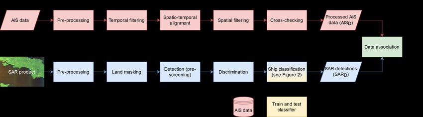
Remote Sens. 2021, 13, 104                                                                                              5 of 26

                                           satellite velocity in metres per second. The AIS-reported position of the ship is
                                           then reckoned by the calculated azimuth shift in its opposite relative azimuth
                                           direction.
                             3.   Spatial filtering:
                                  (a)      The dataset is filtered again according to the spatial extent (or footprint) of the
                                           SAR image.
                                  (b)      AIS data located within the SAR land mask (including the 250 m buffer) are
                                           also removed.
                             4.   Cross-checking:
                                  (a)      The AIS dataset is cross-checked against an open ship database (e.g., ShipAIS [59])
                                           to verify the accuracy of the static data (i.e., length, width and ship type).
                                           Missing or invalid entries are also updated using the International Maritime
                                           Organization (IMO) number to form a more complete dataset for data associa-
                                           tion. (Note that, if the IMO number is not available, then the MMSI number is
                                           used instead.)
                                  It is important to note that interpolation should be carried out before spatially filter-
                             ing the AIS dataset to the footprint of the SAR image; otherwise, some AIS data may be
                             missed or mistakenly included. This is because AIS data initially located outside the foot-
                             print can be subsequently located inside the footprint after interpolation (and vice versa).
                             Equation (1) is a modified version of Equation (1) in [50], which is implemented as an
                             algorithm. Instead of using SAR information, the algorithm is based on information either
                             directly reported by AIS (i.e., SOG and COG) or by what can be derived such as the SAR
                             incidence angle at the AIS-reported position (instead of the SAR detection position). Con-
                             sequently, the azimuth shift process is fast and automatic, which is ideal for the situation
                             where there are a large number of ships in the scene. Following the above procedure, the
                             AIS dataset, AISD , is ready for data association.

                             2.3. Ship Classification
                                   The ship classification model makes predictions on the type of ship in SAR imagery.
                             Specifically, the model is first trained (and tested) on AIS data and then transferred to
                             make predictions on SAR ship detections. This method is known as transfer learning and
                             has shown to be effective for SAR ship classification. This is due to the extensive volume
                             and availability of labelled AIS data, making it ideal for machine learning. The objective
                             is to use class information (i.e., ship type) to maximise the confidence in the association
                             between SAR D and AISD . Figure 2 shows a generalised workflow for generating the ship
                             classification model.

                                        Figure 2. Ship classification model workflow.

                                  A step-by-step procedure is given as follows:
                             1.   Import data: The training data (AISC ) are imported from an AIS database. The
                                  database is typically formed from historical/archive AIS data.
                             2.   Preprocess data: The training data are preprocessed by removing anomalous, missing,
                                  invalid and duplicated entries that may negatively affect the training of the model.
                             3.   Feature selection: Relevant features (or predictors) for use in training the model are
                                  selected (see Table 2). Importantly, since a transfer learning method is used, the
                                  selected features from the AIS data are limited to what can also be extracted and/or
                                  derived from the SAR ship detections.
                             4.   Feature engineering: New features are derived to improve the predictive power of
                                  the model.
Remote Sens. 2021, 13, 104 6 of 26
5. Train model(s): Multiple classification algorithms are iteratively trained and tested
based on the selected and derived features in order to find the best model that predicts
the type of ship.
6. Export model: The best trained model is exported to make ship type predictions on
new data (i.e., SAR ship detections, SAR D ). These predictions are subsequently used
in the data association.
The specific parameters used to generate the ship classification model are given in
Table 2. The classification model is implemented in the MATLAB® environment. The
ship classification model considers only unique ships based on the MMSI number. This is
because only features based on static data (i.e., length, width and aspect ratio) are used
in training the model and so duplicate entries of the same ship can introduce bias. This
results in a relatively simple but powerful classification model. Additionally, geolocation
data (i.e., latitude and longitude) can be used directly in training a model [54] or by first
clustering the data to reduce its dimensionality [60].
The ship classification model implements the Random Undersampling Boosting (RUS-
Boost) algorithm [61]. There are two reasons for selecting this algorithm. Firstly, it is
particularly effective at classifying imbalanced data where some classes in the training data
have significantly fewer observations than other classes. This is commonly exhibited in
AIS data and the distribution or skewness of the classes (ship types) will generally vary
according to the geographical area as well as the time in the shipping season. Secondly,
the RUSBoost algorithm consistently outperforms other ensemble algorithms that do not
implement data sampling techniques (in terms of the true positive rate and false nega-
tive rate for each class), and is computationally less expensive than other hybrid data
sampling/boosting algorithms such as SMOTEBoost [62].
Table 2. Ship classification model parameters.
Parameter Description
Feature selection Ship length (l)
(input features) Ship width (w)
Feature engineering Length-to-width aspect ratio (l/w)
(derived features) Width-to-length aspect ratio (w/l)
Ship type (six classes):
• Cargo
• Fishing
Response • Passenger
• Pleasure
• Tanker
• Tug
Algorithm RUSBoost [61]
Model assessment method k-fold cross-validation (k = 10)
The AIS training data, AISC , totals 20,177 unique entries. Figure 3 shows the number
of unique ships for each response class in the AIS training data. The ‘Other’ and ‘NA (Not
Available)’ ship types as well as those with fewer than one percent of the total number of
observations (e.g., ‘Military’) are excluded from the AIS training data (shown in grey).
Figure 4a,b show the length and width distributions in the AIS training data for each
ship type, respectively. There is a clear distinction between the dimensions of the group
fishing, pleasure and tug ship types and the pair cargo and tanker ship types. In contrast,
the dimensions of the passenger ship type are more uniformly distributed. In order to
find a further distinction between these sub-groups (i.e., discern between a cargo and
tanker), new features or predictors are derived (i.e., feature engineering). Figure 5a,bRemote Sens. 2021, 13, 104 7 of 26
show the width-to-length and length-to-width aspect ratio distributions for each ship type,
respectively.
It is evident from Figure 3 that there is a class imbalance in the training data. In other
words, there is a significant disparity between the number of observations in each class
(or ship type). For example, the pleasure ship type has nearly 11 times the number of
observations compared to the tug ship type. The classification model uses 10-fold cross-
validation to prevent overfitting during training. The trained model results and MATLAB®
model parameters are given in Table 3.
Figure 3. Training data (AISC ) ship type distribution.
(a) (b)
Figure 4. Training data (AISC ) (a) length distribution (grouped into bins of 5 m) and (b) width distribution (grouped into bins of 1 m)
for each ship type.Remote Sens. 2021, 13, 104 8 of 26
(a) (b)
Figure 5. Training data (AISC ) (a) width-to-length aspect ratio (w/l) distribution and (b) length-to-width aspect ratio (l/w) distribution
for each ship type.
Table 3. Trained model results and MATLAB® model parameters.
Model results Value
Accuracy 68.6%
Total misclassification cost 6340
Prediction speed (approx.) 41,000 obs/s
Training time * 16.367 s
Model parameters Value
Preset RUSBoosted Trees
Ensemble method RUSBoost
Learner type Decision tree
Max. number of splits 20
Number of learners 50
Learning rate 0.1
Validation 10-fold cross-validation
* CPU: Intel® Core™ i5-6600K @ 4.40 GHz (16 GB RAM).
2.4. Data Association
The data association of SAR ship detections and AIS data are twofold. Firstly, an m-best
assignment technique is implemented to assign AIS data (AISD ) to SAR ship detections
(SAR D ). Importantly, this technique ranks all the assignments in the order of increasing
cost. The cost is defined as the distance for each AIS-SAR pair, which is computed using the
geodesic distance. The assignments are made by minimising the sum of the total distances
for all possible AIS-SAR pairings. Specifically, the Jonker–Volgenant algorithm [56] is
used to find an optimal solution to the GNN assignment problem. Moreover, the value
selected for m is three meanings for which, for a given SAR ship detection, the top 3-best
assignments in AISD are returned. The performance of this particular technique has been
quantitatively assessed in a previous publication [43].
Secondly, once rank-ordered assignments are made, confidence levels are determined
according to the criteria specified in Table 4. Specifically, the assignments’ geometric (i.e.,Remote Sens. 2021, 13, 104 9 of 26
length and width) and class (i.e., ship type) data are compared, which are considered to
be the most reliable static data fields. The assignments’ geometric data are in agreement
if their absolute difference is within a specified threshold, t. Similarly, the class data are
in agreement if the SAR ship classification matches the one reported by AIS. After the
comparison, the confidence level is determined based on the number of geometric and
class data in agreement. The assignment with the highest confidence level (out of the total
three) is selected as the final assignment. Competing assignments with the same confidence
level are resolved by selecting the highest ranking pair.
Figure 6 shows a conceptual example of how the final assignment is determined. The
top 3-best AIS assignments are returned for a single SAR ship detection. The candidate
assignments are ordered in terms of their rank. The AIS candidates’ reported length, width
and ship type are compared with those of the SAR ship detection. (Recall that the SAR ship
detection’s geometric and class data are determined in Sections 2.1 and 2.3, respectively.)
A confidence level is given to each of the three AIS candidates according to the criteria
specified in Table 4. In the example, the final assignment is A1 . Note that the highest
ranked assignment, A2 , is superseded by the third highest ranked assignment, A1 . The
algorithm correctly updates the final assignment to A1 which has better agreement with
the SAR ship detection.
Figure 6. Final assignment concept.
Table 4. Determination of confidence level.
Confidence Length, l Width, w Ship Type
(SAR Dl − AISDl ≤ tl ) (SAR Dw − AISDw ≤ tw ) SAR DShipType ≡ AISDShipType
Low F F F
T F F
Medium F T F
F F T
T T F
High T F T
F T T
Very High T T T
(T: True; F: False).
3. Results
3.1. Case Study A: English Channel, UK
3.1.1. Product Details
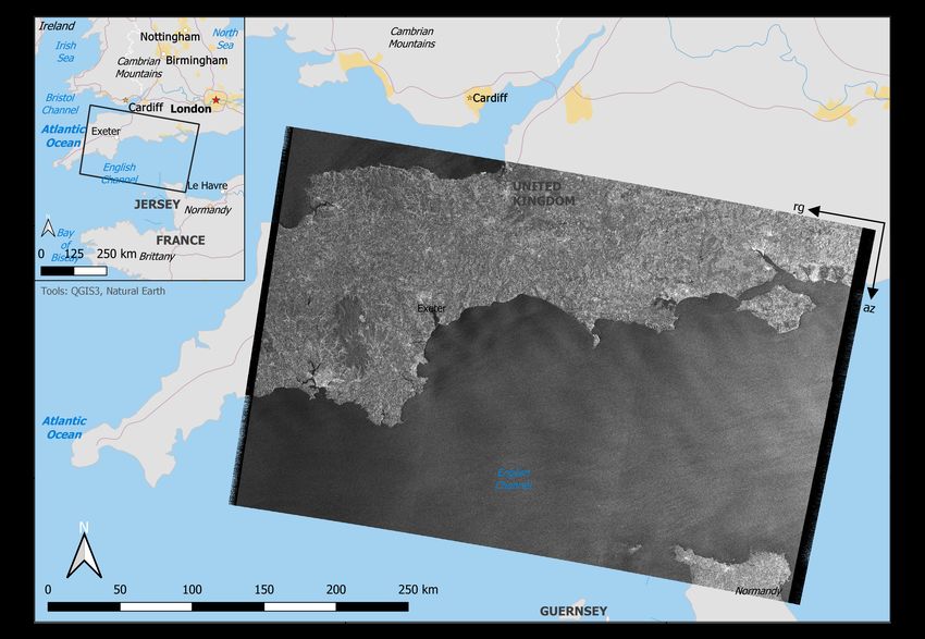
The Sentinel-1 SAR product is acquired in the English Channel, UK. A preview of the
SAR product is shown in Figure 7 with details given in Table 5. The Interferometric Wide
(IW) swath mode of Sentinel-1 is particularly suited for wide-area maritime surveillance
offering a 250 km swath at 20 m by 22 m spatial resolution (multilooked). Figure 8 showsRemote Sens. 2021, 13, 104 10 of 26
the coverage area of the AIS data used for data association (AISD ). The data provided by
LuxSpace Sàrl cover the time period 1 October 2017 to 30 November 2017 (two months),
and comprises terrestrial and satellite-AIS (Sat-AIS) data. The shipping density in the
coverage area is particularly very high with parts showing on average between 10,000
and 100,000 annual vessel transits. The AIS temporal coverage around TSAR (24 October
2017) for the area shown in Figure 8 is also checked to ensure that there is continuous data
reception with no data gaps.
Figure 7. English Channel SAR product (VV polarisation).
Table 5. English Channel SAR product details.
Parameter Description
Datetime (UTC) 2017-10-24T06:23:21.314Z
Instrument SAR-C
Mode IW
Satellite Sentinel-1A
Spatial resolution 20 × 22 m (range × azimuth)
Pass direction Descending
Polarisation VV VH
Product level Level-1
Product type GRD
S1A_IW_GRDH_1SDV_20171024T062321_20171024T062346_
Product identifier
018951_02006B_BCA8Remote Sens. 2021, 13, 104 11 of 26
Figure 8. English Channel AIS coverage area (2 km grid resolution).
3.1.2. Ship Detection
Ship detection follows Section 2.1. Information on the processing parameters is given
in Table 1. In total, SUMO returns 286 detections or targets in the SAR image. After
discrimination, 102 detections are considered to be false alarms. These are subsequently
removed resulting in a new total of 184 detections. The majority of false alarms (58.8%)
arise from an imperfect land mask (see Figure 9).
(a) (b)
Figure 9. English Channel SUMO false alarm examples: (a) imperfect land mask; (b) coastal infrastructure (yellow box) and azimuth
ambiguities (red points).Remote Sens. 2021, 13, 104 12 of 26
3.1.3. AIS Data Processing
The AIS data to be associated with the detections in the SAR image (AISD ) follow
the processes described in Section 2.2. For temporal filtering, a time interval, X, of 40 min
is selected meaning AIS data within 20 min either side of the sensing start time of the
SAR image, TSAR , are considered for association. This value is determined by measuring
the percentage of AIS data that are successfully interpolated to TSAR as a function of
X (see Figure 10). A suitable time interval is one with a high percentage of successful
interpolations for the majority of data whilst keeping the number of unique ships constant
(i.e., limiting the number of ships with a single position in the interpolation as X increases).
Figure 10 shows that, for the time interval X = 40 min, approximately 95% of the AIS
data are successfully interpolated to TSAR (06:23:21 UTC), and little performance is gained
beyond X = 40 min. Figure 11 also shows the average elapsed time between consecutive
timestamps of the same ship, for all ships during October 2017 in the English Channel.
The majority of ships have an average reporting interval in the range of 5–30 min further
supporting a time interval selection of X = 40 min (i.e., TSAR ± 20 min). Figure 12 shows
three visualisations of the interpolation results.
Figure 10. English Channel time interval selection (X = 40 min).
Following interpolation and spatial filtering to the SAR image footprint, AIS data
located within the SAR land mask (including the 250 m buffer) are removed. This results
in a final count of 199 unique ships, of which nine (4.5%) are unsuccessfully interpolated to
TSAR with an average time deviation of 10 min 35 s. Additionally, the average azimuth shift
for the final count is 192.5 m, which is based on ships with a valid and non-zero velocity
(191 total). The azimuth shift is compensated for using Equation (1).
Finally, the dataset is cross-checked against a database. Table 6 gives the number of
missing values in each field both before and after cross-checking the AIS data as well as
the percentage change. After cross-checking, the final dataset has less than 10% of values
missing in each static data field.Remote Sens. 2021, 13, 104 13 of 26
Figure 11. English Channel average reporting interval of the same ship (MMSI), for all ships during
October 2017. (Note that ships with a single timestamp are omitted (total: 3123).)
Figure 12. English Channel interpolation examples.Remote Sens. 2021, 13, 104 14 of 26
Table 6. English Channel missing data before and after cross-checking AIS data (total: 199).
Before After
Change (%)
Data Field # Missing % of Total # Missing % of Total
Length 38 19.2 14 7.1 −12.1
Width 42 21.2 18 9.1 −12.1
Ship type 28 14.1 6 3.0 −11.1
3.1.4. Classification-Aided Data Association
The total number of SAR ship detections (SAR D ) and unique AIS data points (AISD ),
as well as their respective number of assignments and unassignments, are given in Table 7.
Figure 13 shows a visualisation of these results. The agreement in the assignments’ geometric
and class data is also given in Table 7. The selected geometric thresholds (see Table 4) are
tl = 25 m (2.5 pixels) and tw = 10 m (1 pixel) for the length and width, respectively.
Table 7. English Channel total number of (top) assignments and unassignments (bottom) features
in agreement.
SAR D AISD
Total 184 199
Assigned 152
% of Total 82.6 76.4
Unassigned 32 47
% of Total 17.4 23.6
Assigned Feature # of matches
Length (valid: 146) 55 (37.7%)
152 Width (valid: 141) 129 (91.5%)
Ship type (valid: 135) 34 (25.2%)
Figure 14a shows the estimated SAR length returned by the SUMO algorithm plot-
ted against the reported AIS length for each assignment. The SAR-estimated lengths
show moderate agreement with AIS-reported lengths greater than 100 m. Conversely,
SAR-estimated lengths are considerably overestimated for AIS-reported lengths below
100 m, especially at 20 m (approximately). Figure 14b shows a similar plot for widths.
The SAR-estimated widths show a consistent overestimation for all AIS-reported widths.
The overestimation by the SUMO algorithm is corrected for by establishing the relationship
between the estimated SAR width and AIS-reported width (of the form y = mx + c). This is
done using linear regression; specifically, a robust least-squares fit with bisquare weights is
used to estimate the parameters (i.e., gradient, m and intercept, c) of the relationship. The
inverse of this relationship is used to update the estimated SAR width values. Figure 14c
shows the updated values of the estimated SAR width plotted against the reported AIS
width for each assignment. In comparison to Figure 14b, the gradient is now very close to
an ideal value of one.
The general overestimation in SAR-estimated dimensions can be explained by the
variability in a target’s SAR signature [63]. For example, some overestimations are likely a
consequence of azimuth blurring, which is a form of motion-induced distortion sometimes
found in SAR imagery [48]. This is caused by the motion of a target such as a ship relative to
the radar (i.e., moving linearly in the azimuth direction). (This is a similar effect to azimuth
shift where moving targets in the range direction appear displaced in azimuth.) Reportedly,
this blurring can be of the order of 100 m giving rise to significant overestimations of the
ship’s dimensions, especially for small ships [19,64].Remote Sens. 2021, 13, 104 15 of 26
Figure 13. English Channel data association.
A histogram of the confidence levels of the 152 assignments is shown in Figure 15a.
In total, 34 assignments (25.2%) (out of a maximum of 135 AIS data points with a valid
ship type) received an improved confidence level due to a match in their ship type. These
assignments would have otherwise had a lower confidence level if ship classification were
not implemented.
In total, 47 AIS data points (23.6%) and 32 SAR detections (17.4%) are unassigned.
After visually inspecting the SAR signatures of the unassigned AIS data points in the SAR
image, it is observed that:
• Four (4) are due to a discrepancy between the SAR footprint and the SAR image.
The main reason is the SAR image contains noise (or artefacts) at its borders (visible
in Figure 7). (This noise is common to Sentinel-1 Level-1 GRD products after being
processed from RAW data.) The extent of the SAR footprint includes these areas of
border noise where AIS data points may be located but no SAR detections.
• Seven (7) are unsuccessfully interpolated to TSAR , meaning their true positions have a
greater associated uncertainty and are less likely to be assigned.
• 11 are moored to structures such as piers and oil terminals located within ports and
harbours (located outside the land mask). These structures merge with or deform the
SAR signature in such a way that leads to no SAR detection.
• 20 are either below the selected SUMO detection threshold or have a very weak SAR
signature that is below the limit of detectability of the SAR sensor. These are generally
small ships. For example, the average ship length of the 20 unassigned AIS data points
is 16.3 m where most are fishing vessels.
There are 32 unassigned SAR detections. After visually inspecting the unassigned SAR
detections in the SAR image, it is observed that 14 are false alarms which have been missedRemote Sens. 2021, 13, 104 16 of 26
by initial inspection (see Section 3.1.2). The remaining 18 unassigned SAR detections are
thought to be ‘dark’ ships.
(a)
(b) (c)
Figure 14. English Channel estimated SAR (a) length; (b) width; (c) updated width; against reported AIS for each assignment.
Figure 15b shows the distribution of AIS-SAR assignment (or matching) distances.
The average distance is 160.9 m with the majority having a distance less than 100 m.
This discrepancy can be explained by small errors in the interpolation and azimuth shift
compensation processes and, to a lesser extent, georeferencing errors introduced from the
SAR coordinate transformation. Additionally, both sensors have an associated uncertainty
in their geolocation accuracy. The Sentinel-1 Interferometric Wide (IW) swath modeRemote Sens. 2021, 13, 104 17 of 26
typically has a geolocation accuracy of 7 m [65], while AIS indicates the position accuracy
as either ‘high’ (≤10 m) or ‘low’ (>10 m, default) [1].
Three AIS-SAR assignments have a distance greater than one kilometre. One is from
removing a SAR detection incorrectly identified as an azimuth ambiguity by the SUMO
algorithm. This caused the AIS data point to match with a SAR detection located at a much
greater distance. The other two are related to the interpolation process with one being
unsuccessfully interpolated to TSAR (time deviation of 18 min 28 s), and the other having
an undulation that overshoots at TSAR . The average matching distance is 133.0 m excluding
these three outliers.
(a) (b)
Figure 15. English Channel (a) AIS-SAR assignment confidence levels and (b) distribution of assignment distances.
3.2. Case Study B: The Solent, UK
3.2.1. Product Details
The ICEYE-X2 SAR product is acquired in the Solent, UK. A preview of the SAR
product is shown in Figure 16 with details given in Table 8. The Stripmap imaging mode
is particularly suited for focused maritime surveillance offering a 30 km swath at 3 m
by 3 m spatial resolution (multilooked). The coverage area of the AIS data used for data
association (AISD ) is the same as the SAR footprint. The data provided by Spire Maritime
covers 24 h on 30 October 2020 and comprises of terrestrial and satellite-AIS (Sat-AIS) data.
Table 8. The Solent SAR product details.
Parameter Description
Datetime (UTC) 2020-10-30T10:43:22.739
Mode Stripmap
Satellite ICEYE-X2
Spatial resolution 3 × 3 m (range × azimuth)
Pass direction Descending
Polarisation VV
Product type GRD
Product identifier ICEYE_X2_GRD_SM_36769_20201030T104322Remote Sens. 2021, 13, 104 18 of 26
Figure 16. The Solent SAR product (VV polarisation).
3.2.2. Ship Detection
The SUMO ship detection software does not currently support ICEYE products;
therefore, ship detection is carried out in the Sentinel Application Platform (SNAP) which
uses a CFAR algorithm. The SNAP processing parameters are given in Table 9.
Table 9. SNAP: SAR processing parameters.
Parameter Description
Application SNAP (version 7.0)
Calibration Output sigma0 band
Land mask OpenStreetMap (50 m buffer)
Algorithm (detector) Two-parameter CFAR
Target Window Size (m): 20
Guard Window Size (m): 500
Adaptive thresholding
Background Window Size (m): 800
PFA: 10−7
Object dimension threshold:
Object discrimination Min. Target Size (m): 10
Max. Target Size (m): 600Remote Sens. 2021, 13, 104 19 of 26
3.2.3. AIS Data Processing
The AIS data processing follows a similar process to Section 3.1.3. For temporal
filtering a time interval, X, of 60 min is selected. Following interpolation and spatial
filtering, a final count of 45 unique ships are returned, of which two are unsuccessfully
interpolated to TSAR (10:43:22 UTC).
3.2.4. Classification-Aided Data Association
The total number of SAR ship detections (SAR D ) and unique AIS data points (AISD ),
as well as their respective number of assignments and unassignments, are given in Table 10.
Figure 17 shows a visualisation of these results. The agreement in the assignments’ geomet-
ric and class data are also given in Table 10. The selected geometric thresholds (see Table 4)
are tl = 12.5 m (5 pixels) and tw = 7.5 m (3 pixels) for the length and width, respectively.
Figure 17. The Solent data association.
Figure 18a shows the estimated SAR length plotted against the reported AIS length
for each assignment. The SAR-estimated lengths show good agreement with AIS-reported
lengths. Figure 18b shows a similar plot for widths. Similarly, the SAR-estimated widths
show a good agreement with AIS-reported widths.
A histogram of the confidence levels of the 21 assignments is shown in Figure 19a. The
majority of assignments received a ‘Very High’ confidence level. In total, 13 assignments
(76.5%) (out of a maximum of 17 AIS data points with a valid ship type) received an
improved confidence level due to a match in their ship type. These assignments would
have otherwise had a lower confidence level if ship classification were not implemented.
In total, 24 AIS data points (53.3%) and five SAR detections (19.2%) are unassigned.
After visually inspecting the SAR signatures of the unassigned AIS data points in theRemote Sens. 2021, 13, 104 20 of 26
SAR image, it is observed that: three (3) are moored to structures (such as a tug pontoon)
that deform the SAR signature in such a way that leads to no SAR detection; and 21 are
small ships, the majority of which are pleasure boats constructed from fiberglass that are
particularly difficult to detect in SAR imagery. These ships have a very weak SAR signature
that is at or below the level of the sea clutter. Furthermore, there are five (5) unassigned
SAR detections. After visually inspecting the unassigned SAR detections in the SAR image,
it is observed that all five (5) are ‘dark’ ships that are not transmitting AIS. These ships are
located east of the Isle of Wight within the range of terrestrial AIS receiving stations (see
Figure 17), and are of a size and predicted class that should be transmitting AIS.
Figure 19b shows the distribution of AIS-SAR assignment (or matching) distances.
The average distance is 115.6 m with the majority having a distance less than 100 m.
Table 10. The Solent total number of (top) assignments and unassignments (bottom) features in agree-
ment.
SAR D AISD
Total 26 45
Assigned 21
% of Total 80.8 46.7
Unassigned 5 24
% of Total 19.2 53.3
Assigned Feature # of matches
Length (valid: 20) 18 (90.0%)
21 Width (valid: 20) 18 (90.0%)
Ship type (valid: 17) 13 (76.5%)
(a) (b)
Figure 18. The Solent estimated SAR (a) length and (b) width against reported AIS for each assignment.Remote Sens. 2021, 13, 104 21 of 26
(a)
(b)
Figure 19. The Solent (a) AIS-SAR assignment confidence levels and (b) distribution of assignment distances.
4. Discussion
4.1. Effectiveness of Rank-Ordered Assignment
For Case Study A (English Channel, UK), the results demonstrate a high level of
correspondence between the data with 82.6% of SAR ship detections and 76.4% of AIS data
points being assigned. This is a highly satisfactory result, especially when considering the
challenges of wide-area and large-scale data association in very dense shipping environ-
ments such as the English Channel. The same SAR product and AIS data are used in the
‘English Channel Test Case’ in [21], which allows for a broad comparison of the results. For
example, in this work, the AIS data processing returns 199 AIS data points compared to
the 140 points in [21]. This is thought to be primarily due to the empirical determination of
the time interval, X. Additionally, AIS-SAR assignments with shorter assignment distances
are achieved (see Figure 15b) due to azimuth image shift compensation and accurate in-
terpolation. Typically, it is difficult to carry out azimuth image shift compensation for a
large number of ships; however, an automatic and scalable algorithm based on the SAR
incidence angle at the AIS-reported position has been used here. Overall, a higher AIS-SAR
assignment with good confidence values is achieved.
For Case Study B (The Solent, UK), 80.8% of SAR ship detections and 46.7% of AIS data
points are assigned. The low number of unassigned SAR ship detections exhibited in both
case studies allows for a more efficient investigation into the reasons why detected ships
may not be transmitting AIS. The inference of behaviour from ‘dark’ ships is a compelling
research area worth further investigation. Some ships, however, are not detected in the SAR
image demonstrating a limitation of the SAR ship detection. The majority of unassigned
AIS data points in Case Study B are pleasure boats constructed from fiberglass that are
particularly difficult to detect in SAR imagery. Therefore, alternative SAR ship detectors
that focus on the detection of small, non-metallic ships may prove to be useful [66]. The
fusion workflow (see Figure 1) is highly modular meaning that it is relatively simple to
implement alternative SAR ship detectors.
The accurate discrimination of SAR false alarms also has a great effect on the data
association performance. For example, in Case Study A (English Channel, UK), the majority
of false alarms arise from an imperfect land mask or are caused by coastal infrastructure
and azimuth ambiguities. Therefore, improvements in the discrimination of SAR false
alarms, such as the use of highly-accurate land masks, will directly improve the overall
data association between SAR and AIS. In this work, optical satellite imagery is used to
identify fixed structures; however, the use of repeat–pass SAR imagery is an effectiveRemote Sens. 2021, 13, 104 22 of 26
alternative method to identify specific types of SAR false alarms (e.g., range ambiguities
and fixed structures) [5,19].
The rank-ordered assignment algorithm demonstrated its robustness by automati-
cally correcting itself after determining the top-best assignments, corroborating previous
simulation results [43]. Figure 20 shows a scenario similar to the conceptual example
shown in Figure 6. Initially, the algorithm returns the assignments shown in Figure 20a,
which are considered the top-best assignments (i.e., rank equal to one). When considering
the geometric and class information, the algorithm correctly updates to the third-best
assignments shown in Figure 20b which have better agreement.
(a) (b)
Figure 20. Rank-ordered assignment algorithm correctly updated from (a) rank 1 to (b) rank 3 AIS-SAR assignments
(AIS data points shown in red and SAR ship detections shown in blue).
4.2. Effectiveness of Ship Classification
The SAR ship classification model based on AIS transfer learning shows improvement
in the confidence level of the assignments. For Case Study A (English Channel, UK), 25.2%
of the AIS-SAR assignments have a matching ship type, thereby directly improving the
confidence level for these assignments. Similarly, 37.7% received an improved confidence
level due to a match in their length and 91.5% due to a match in their width. In contrast,
for Case Study B (the Solent, UK), 76.5% of the AIS-SAR assignments have a matching ship
type. Similarly, 90.0% received an improved confidence level due to a match in both their
length and width.
It is evident that the ship classification model performs better in Case Study B which
uses a higher spatial resolution SAR image. This is because more accurate estimates of
SAR-derived ship dimensions are obtained leading to better predictions from the model
(see Figure 18). The model is also effective over a wider range of ship types (i.e., six classes)
for higher spatial resolution compared to previous studies [53,54]. This includes the model
correctly predicting the ship classes: cargo, tanker, passenger and tug. For the lower spatial
resolution SAR image in Case Study A, an empirical correction has been applied to account
for the observed overestimation in ship width returned by the SUMO algorithm with
improvements shown (see Figure 14c). However, to improve the estimates of SAR-derived
ship dimensions in Sentinel-1 (IW mode) imagery, other more sophisticated SAR ship size
estimation techniques are needed (e.g., [63,67]).
As the geometric data are the only transferable features used from AIS, future con-
siderations and potential improvements to the ship classification include finding other
transferable features. For example, clustering involves using the location of the vessel in
latitude and in longitude as an input feature in order to improve the model’s predictive
power [60]. Additionally, the use of contextual information involves using the knowledge
that the distribution of ship types vary depending on the geographical area. For example,
in Southern California, typically a high amount of pleasure craft are observed, whereas,
in Southern Louisiana (Gulf of Mexico), a much lower number is observed and tug shipsRemote Sens. 2021, 13, 104 23 of 26
make up one of the majority classes. Alongside transferring AIS knowledge, this a priori
knowledge can be used to improve SAR ship classification performance.
5. Conclusions
A classification-aided data association technique is proposed and evaluated in very
dense shipping environments, including the English Channel and The Solent, UK. The
research method demonstrates a high level of correspondence between the SAR and AIS
data with good confidence values. In particular, the high correlation of SAR ship detections
means that it is more practical to investigate ‘dark’ ships. The SAR ship classification uses
a transfer learning method and its performance is evaluated using two SAR products of
different spatial resolution. It is shown that implementing ship classification in conjunction
with a rank-ordered assignment technique improves the confidence in the data association.
The class information helps reduce ambiguity in the rank-ordered assignments, thereby
providing a robust match between the data. The transfer learning method shows significant
improvement in higher spatial resolution SAR imagery, where the percentage of AIS-
SAR assignments with a match in their ship type increased from 25.2% in the Sentinel-1
Interferometric Wide (IW) swath mode product to 76.5% for the ICEYE-X2 Stripmap mode
product. Therefore, future work will explore the implementation of more accurate SAR
ship size estimation techniques for lower spatial resolution SAR imagery. The data fusion
framework described in this paper can also be extended to include other sources of data
(e.g., optical, thermal infrared, etc.) which support applications that contribute to maritime
safety and security.
Author Contributions: The first author, M.R., was responsible for developing the methodology,
implementing the software, validating the results and writing the original draft. The research was
supervised by the second author, R.G., who provided regular feedback and reviewed the original
draft. All authors have read and agreed to the published version of the manuscript.
Funding: This research was funded by Surrey Satellite Technology Limited (SSTL) as part of a stu-
dentship.
Institutional Review Board Statement: Not applicable.
Informed Consent Statement: Not applicable.
Data Availability Statement: The Sentinel-1 SAR product presented in this study is openly available
at the Copernicus Open Access Hub.
Acknowledgments: The authors would like to thank LuxSpace Sàrl for freely providing the AIS
dataset for the English Channel case study. They would also like to thank Spire Maritime for freely
providing the AIS dataset for the Solent case study.
Conflicts of Interest: The authors declare no conflict of interest.
References
1. ITU Radiocommunication Sector (ITU-R). Technical Characteristics for An Automatic Identification System Using Time-Division
Multiple Access in The Vhf Maritime Mobile Band; Recommendation ITU-R M.1371-5; International Telecommunication Union (ITU):
Geneva, Switzerland, 2014.
2. Brusch, S.; Lehner, S.; Fritz, T.; Soccorsi, M.; Soloviev, A.; van Schie, B. Ship Surveillance With TerraSAR-X. IEEE Trans. Geosci.
Remote Sens. 2011, 49, 1092–1103. [CrossRef]
3. Vachon, P.W.; Kabatoff, C.; Quinn, R. Operational ship detection in Canada using RADARSAT. In Proceedings of the 2014 IEEE
Geoscience and Remote Sensing Symposium, Quebec City, QC, Canada, 13–18 July 2014; pp. 998–1001. [CrossRef]
4. Velotto, D.; Bentes, C.; Tings, B.; Lehner, S. First, Comparison of Sentinel-1 and TerraSAR-X Data in the Framework of Maritime
Targets Detection: South Italy Case. IEEE J. Ocean. Eng. 2016, 41, 993–1006. [CrossRef]
5. Santamaria, C.; Alvarez, M.; Greidanus, H.; Syrris, V.; Soille, P.; Argentieri, P. Mass Processing of Sentinel-1 Images for Maritime
Surveillance. Remote Sens. 2017, 9, 678. [CrossRef]
6. Lehner, S.; Brusch, S.; Fritz, T. Ship surveillance by joint use of SAR and AIS. In Proceedings of the OCEANS 2009-EUROPE,
Bremen, Germany, 11–14 May 2009; pp. 1–5. [CrossRef]Remote Sens. 2021, 13, 104 24 of 26
7. Posada, M.; Greidanus, H.; Alvarez, M.; Vespe, M.; Cokacar, T.; Falchetti, S. Maritime awareness for counter-piracy in the Gulf of
Aden. In Proceedings of the 2011 IEEE International Geoscience and Remote Sensing Symposium, Vancouver, BC, Canada, 24–29
July 2011; pp. 249–252. [CrossRef]
8. Longépé, N.; Hajduch, G.; Ardianto, R.; de Joux, R.; Nhunfat, B.; Marzuki, M.I.; Fablet, R.; Hermawan, I.; Germain, O.; Subki, B.A.;
et al. Completing fishing monitoring with spaceborne Vessel Detection System (VDS) and Automatic Identification System (AIS)
to assess illegal fishing in Indonesia. Mar. Pollut. Bull. 2018, 131, 33–39. [CrossRef] [PubMed]
9. Rowlands, G.; Brown, J.; Soule, B.; Boluda, P.T.; Rogers, A.D. Satellite surveillance of fishing vessel activity in the Ascension
Island Exclusive Economic Zone and Marine Protected Area. Mar. Policy 2019, 101, 39–50. [CrossRef]
10. Kurekin, A.A.; Loveday, B.R.; Clements, O.; Quartly, G.D.; Miller, P.I.; Wiafe, G.; Adu Agyekum, K. Operational Monitoring of
Illegal Fishing in Ghana through Exploitation of Satellite Earth Observation and AIS Data. Remote Sens. 2019, 11, 293. [CrossRef]
11. Park, J.; Lee, J.; Seto, K.; Hochberg, T.; Wong, B.A.; Miller, N.A.; Takasaki, K.; Kubota, H.; Oozeki, Y.; Doshi, S.; et al. Illuminating
dark fishing fleets in North Korea. Sci. Adv. 2020, 6. [CrossRef]
12. Uiboupin, R.; Raudsepp, U.; Sipelgas, L. Detection of oil spills on SAR images, identification of polluters and forecast of the
slicks trajectory. In Proceedings of the 2008 IEEE/OES US/EU-Baltic International Symposium, Tallinn, Estonia, 27–29 May 2008;
pp. 1–5. [CrossRef]
13. Longépé, N.; Mouche, A.; Goacolou, M.; Granier, N.; Carrere, L.; Lebras, J.; Lozach, P.; Besnard, S. Polluter identification with
spaceborne radar imagery, AIS and forward drift modeling. Mar. Pollut. Bull. 2015, 101, 826–833. [CrossRef]
14. Garello, R.; Kerbaol, V. Oil pollution monitoring: An integrated approach. In Proceedings of the 2017 IEEE Workshop on
Environmental, Energy, and Structural Monitoring Systems (EESMS), Milan, Italy, 24–25 July 2017; pp. 1–6. [CrossRef]
15. English, J.; Hewitt, R.; Power, D.; Tunaley, J. ICE-SAIS — Space-based AIS and SAR for improved Ship and Iceberg Monitoring.
In Proceedings of the 2013 IEEE Radar Conference (RadarCon13), Ottawa, ON, Canada, 29 April–3 May 2013; pp. 1–6. [CrossRef]
16. Marino, A.; Hajnsek, I. Statistical Tests for a Ship Detector Based on the Polarimetric Notch Filter. IEEE Trans. Geosci. Remote Sens.
2015, 53, 4578–4595. [CrossRef]
17. Touzi, R.; Vachon, P.W. RCM Polarimetric SAR for Enhanced Ship Detection and Classification. Can. J. Remote Sens. 2015,
41, 473–484. [CrossRef]
18. Iervolino, P.; Guida, R. A Novel Ship Detector Based on the Generalized-Likelihood Ratio Test for SAR Imagery. IEEE J. Sel. Top.
Appl. Earth Obs. Remote Sens. 2017, 10, 3616–3630. [CrossRef]
19. Greidanus, H.; Alvarez, M.; Santamaria, C.; Thoorens, F.X.; Kourti, N.; Argentieri, P. The SUMO Ship Detector Algorithm for
Satellite Radar Images. Remote Sens. 2017, 9, 246. [CrossRef]
20. Sandirasegaram, N.; Vachon, P.W. Validating Targets Detected by SAR Ship Detection Engines. Can. J. Remote Sens. 2017,
43, 451–454. [CrossRef]
21. Pelich, R.; Chini, M.; Hostache, R.; Matgen, P.; Lopez-Martinez, C.; Nuevo, M.; Ries, P.; Eiden, G. Large-Scale Automatic Vessel
Monitoring Based on Dual-Polarization Sentinel-1 and AIS Data. Remote Sens. 2019, 11, 1078. [CrossRef]
22. Margarit, G.; Barba Milanés, J.A.; Tabasco, A. Operational Ship Monitoring System Based on Synthetic Aperture Radar Processing.
Remote Sens. 2009, 1, 375–392. [CrossRef]
23. Margarit, G.; Tabasco, A. Ship Classification in Single-Pol SAR Images Based on Fuzzy Logic. IEEE Trans. Geosci. Remote Sens.
2011, 49, 3129–3138. [CrossRef]
24. Xing, X.; Ji, K.; Zou, H.; Chen, W.; Sun, J. Ship Classification in TerraSAR-X Images With Feature Space Based Sparse Representa-
tion. IEEE Geosci. Remote Sens. Lett. 2013, 10, 1562–1566. [CrossRef]
25. Wang, C.; Zhang, H.; Wu, F.; Jiang, S.; Zhang, B.; Tang, Y. A Novel Hierarchical Ship Classifier for COSMO-SkyMed SAR Data.
IEEE Geosci. Remote Sens. Lett. 2014, 11, 484–488. [CrossRef]
26. Fernandez Arguedas, V.; Velotto, D.; Tings, B.; Greidanus, H.; Bentes da Silva, C.A. Ship classification in high and very high
resolution satellite SAR imagery. In Proceedings of the Security Research Conference, 11th Future Security, Berlin, Germany,
13–14 September 2016; pp. 347–354.
27. Jiang, M.; Yang, X.; Dong, Z.; Fang, S.; Meng, J. Ship Classification Based on Superstructure Scattering Features in SAR Images.
IEEE Geosci. Remote Sens. Lett. 2016, 13, 616–620. [CrossRef]
28. Huang, L.; Liu, B.; Li, B.; Guo, W.; Yu, W.; Zhang, Z.; Yu, W. OpenSARShip: A Dataset Dedicated to Sentinel-1 Ship Interpretation.
IEEE J. Sel. Top. Appl. Earth Obs. Remote Sens. 2018, 11, 195–208. [CrossRef]
29. Hou, X.; Ao, W.; Song, Q.; Lai, J.; Wang, H.; Xu, F. FUSAR-Ship: Building a high-resolution SAR-AIS matchup dataset of Gaofen-3
for ship detection and recognition. Sci. China Inf. Sci. 2020, 63. [CrossRef]
30. Song, J.; Kim, D.J.; Kang, K.M. Automated Procurement of Training Data for Machine Learning Algorithm on Ship Detection
Using AIS Information. Remote Sens. 2020, 12, 1443. [CrossRef]
31. Grasso, R.; Mirra, S.; Baldacci, A.; Horstmann, J.; Coffin, M.; Jarvis, M. Performance Assessment of a Mathematical Morphology
Ship Detection Algorithm for SAR Images through Comparison with AIS Data. In Proceedings of the 2009 Ninth International
Conference on Intelligent Systems Design and Applications, Pisa, Italy, 30 November–2 December 2009; pp. 602–607. [CrossRef]
32. Gurgel, K.; Schlick, T.; Horstmann, J.; Maresca, S. Evaluation of an HF-radar ship detection and tracking algorithm by comparison
to AIS and SAR data. In Proceedings of the 2010 International WaterSide Security Conference, Carrara, Italy, 3–5 November 2010;
pp. 1–6. [CrossRef]You can also read