A Constrained Probabilistic Petri Net Framework for Human Activity Detection in Video
←
→
Page content transcription
If your browser does not render page correctly, please read the page content below
IEEE TRANSACTIONS ON MULTIMEDIA                                                                                                          1

    A Constrained Probabilistic Petri Net Framework
        for Human Activity Detection in Video
                            Massimiliano Albanese, Rama Chellappa, Fellow, IEEE
          Vincenzo Moscato, Antonio Picariello, V.S. Subrahmanian, Pavan Turaga *, Student Member
                                     and Octavian Udrea, Student Member

   Abstract— EDICS code: 4-KEEP, 2-ALAR. Recognition of                 occlusions, noise etc. and b) at the higher-level, activities in
human activities in restricted settings such as airports, parking       such settings are usually characterized by complex multi-agent
lots and banks is of significant interest in security and automated     interaction, and c) the same semantic activity can be performed
surveillance systems. In such settings, data is usually in the
form of surveillance videos with wide variation in quality and          in several variations which may not conform to strict statistical
granularity. Interpretation and identification of human activities      or syntactic constraints.
requires an activity model that is a) rich enough to handle                In real life scenarios, one usually has some prior knowledge
complex multi-agent interactions, b) is robust to uncertainty           of the type of activities that occur in a given domain and their
in low-level processing and c) can handle ambiguities in the            corresponding semantic structure. In addition, one may also
unfolding of activities. Efficient inference algorithms based on
the activity model then provide means to accomplish the tasks           have access to a limited training set, which in most cases
of activity recognition and anomaly detection. Toward this end,         is not exhaustive. Thus, there is a need for approaches that
we present a computational framework for human activity                 can leverage available domain knowledge to design semantic
representation based on Petri nets. We propose an extension –           activity models and yet retain the robustness of the statistical
Probabilistic Petri Nets (PPN)- and show how this model is well         approaches. The fusion of these disparate approaches – sta-
suited to address each of the above requirements in a wide variety
of settings. Then, we focus on answering two types of questions:        tistical, structural and knowledge based – has not yet been
(i) what are the minimal sub-videos in which a given activity is        fully realized and has only been gaining attention in recent
identified with a probability above a certain threshold and (ii)        years. Our approach falls in this category that combines these
for a given video, which activity from a given set occurred with        approaches – where we exploit domain knowledge to create
the highest probability ? We provide the PPN-MPS algorithm for          rich and expressive models for activities based on the Petri net
the first problem, as well as two different algorithms (naivePPN-
MPA and PPN-MPA) to solve the second. Our experimental                  formalism, and augment the standard Petri net model with a
results on a dataset consisting of bank surveillance videos and         probabilistic extension to handle (a) ‘noise’ in the labeling of
an unconstrained TSA tarmac surveillance dataset show that our          video data, (b) inaccuracies in vision algorithms and (c) allow
algorithms are both fast and provide high quality results.              for departures from a hard-coded activity model.
                                                                           Based on this activity model, given a segment s of a video,
                                                                        we can then define a probability that the segment s contains
                       I. I NTRODUCTION
                                                                        an instance of the activity in question. We then provide fast
   The task of designing algorithms that can analyze human              algorithms to answer two kinds of queries. The first type of
activities in video sequences has been an active field of               query tries to find minimal (i.e. the shortest possible) clips of
research during the past ten years. Nevertheless, we are still          video that contain a given event with a probability exceeding
far from a systematic solution to the problem. The analysis             a specified threshold — we call these Threshold Activity
of activities performed by humans in restricted settings is of          Queries. The second type of query takes a portion of a video
great importance in applications such as automated security             (the part seen thus far) and a set of activities, and tries to find
and surveillance systems. There has been significant interest           the activity that most likely occurred in the video — we call
in this area where the challenge is to automatically recognize          these Activity Recognition Queries.
the activities occurring in a camera’s field of view and detect
abnormalities. The practical applications of such a system
could include airport tarmac monitoring, monitoring of ac-              A. Prior Related Work
tivities in secure installations, surveillance in parking lots etc.        The study and analysis of human activities has a wide and
The difficulty of the problem is compounded by several factors          rich literature. On the one hand there has been significant effort
- a) at the lower-level, unambiguous detection of primitive             to build algorithms that can learn patterns from training data -
actions can be challenging due to changes in illumination,              which can be broadly classified as statistical techniques - and
                                                                        on the other hand, there are the model-based or knowledge-
   Authors listed in alphabetical order. V. Moscato and A. Picariello
are with the Università di Napoli, Federico II, Napoli, Italy,         based approaches represent activities at a higher level of
Email:     {vmoscato, picus}@unina.it.       Massimiliano  Albanese,    abstraction. A recent survey of computational approaches for
Rama Chellappa, V.S. Subrahmanian, Pavan Turaga and Octavian            activity modeling and recognition may be found in [1].
Udrea are with the Institute for Advanced Computer Studies,
University of Maryland, College Park, MD 20742. Email:                     Statistical approaches: A large body of work in the ac-
{albanese, rama, vs, pturaga, udrea}@umiacs.umd.edu.                    tivity recognition area builds on statistical pattern recognition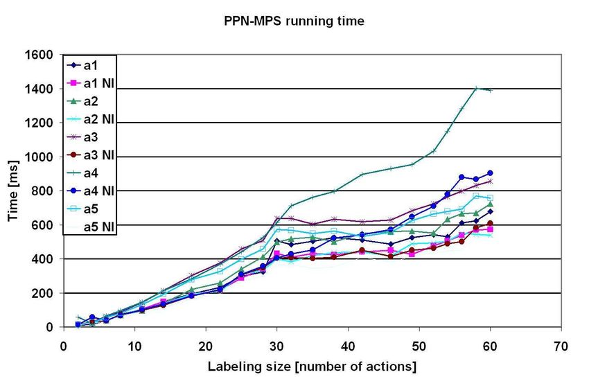
2                                                                                                          IEEE TRANSACTIONS ON MULTIMEDIA

methods. Hidden Markov Models (HMMs) [2], [3] and its               Attribute grammars have also been used to combine syntactic
extensions such as Coupled Hidden Markov Models (CHMMs)             and statistical models for visual surveillance applications in
[4] have been used for activity recognition. Bobick and Davis       [17]. Though grammar based approaches present a sound theo-
[5] developed a method for characterizing human actions based       retical tool for behavior modeling, in practice, the specification
on the concept of “temporal templates”. Kendall’s shape theory      of the grammar itself becomes difficult for complex activities.
has been used to model the interactions of a group of people        Further, it is difficult to model behaviors such as concurrency,
and objects by Vaswani et al [6]. Statistical approaches such as    synchronization, resource sharing etc using grammars. Petri
these require a training phase in which models are learnt from      nets on the other hand are well suited for these tasks and have
training exemplars. This inherently assumes the existence of a      been traditionally used in the field of compiler design and
rich training set which encompasses all possible variations in      hybrid systems. A probabilistic version of Petri nets based
which an activity may be performed. But, in real life situations,   on particle filters was presented by Lesire and Tessier [18]
one is not provided with an exhaustive training set. Moreover,      for flight monitoring. Possibilistic Petri nets which combine
it is not possible to anticipate the various ways an activity       possibility logic with Petri nets have been used for modeling
may be performed. Statistical techniques do not model the           of manufacturing systems by [19]. In computer vision, activity
semantics of activities and may fail to recognize the same          recognition using Petri nets has been investigated by Ghanem
activity performed in a different manner. They are also not well    et al [15] and Castel et al [14]. However, they do not deal
suited to model the complex behaviors such as concurrence,          with probabilistic modeling and detection, instead relying on
synchronization and multiple instances of activities.               perfect accuracy in the lower levels.
   Structural approaches: Unlike the statistical methods               It is important to note that the aforementioned papers do
which assume the availability of a training set, these methods      not explicitly address the following problems: (i) developing
usually rely on hand-crafted models from experts or analysts.       efficient algorithms to find all minimal segments of a video
Since the models are hand-crafted, they are often intuitive         that contain a given activity with a probability exceeding a
and can be related to the semantic structure of the activity. A     given threshold and (ii) developing efficient algorithms to find
method for generating high-level descriptions of traffic scenes     the activity that is most likely (from a given set of activities)
was implemented by Huang et al. using a dynamic Bayes               in a given video segment.
networks (DBN) [7], [8]. Hongeng and Nevatia [9] proposed a            Contributions: First, we introduce a probabilistic Petri
method for recognizing events involving multiple objects using      Net representation of complex activities based on atomic
temporal logic networks. Context free grammars have been            actions which are recognizable by image understanding al-
used by [10] to recognize sequences of discrete events. Ivanov      gorithms. The next major contribution is the PPN-MPS1 algo-
and Bobick [11] used Stochastic Context Free Grammars               rithm to answer threshold queries. Our third major contribution
(SCFG) to represent human activities in surveillance videos. In     is the naivePPN-MPA and PPN-MPA2 algorithms to solve
an approach related to that presented in this paper, Albanese et    activity recognition queries. We evaluate these algorithms
al. [12] use stochastic automata to model activities and provide    theoretically as well as experimentally (in Section VI) on two
algorithms to find subvideos matching the activities. Shet,         third party datasets consisting of staged bank robbery videos
Harwood and Davis [13] have proposed using a Prolog based           [20] and unconstrained airport tarmac surveillance videos and
reasoning engine to model and recognize activities in video.        provide evidence that the algorithms are both efficient and
Castel, Chaudron and Tessier [14] developed a system for            yield high-quality results.
high-level interpretation of image sequences based on deter-           Organization of paper: First, in Section II we define
ministic Petri nets. Deterministic Petri nets have also been used   probabilistic Petri nets (PPN) and discuss representation of
by Ghanem et al [15] as a tool for querying of surveillance         complex activities using the PPN framework. Then, we present
videos. Though structural methods have distinct advantages          efficient algorithms to solve the Most Probable Subsequence
over statistical techniques in terms of representative and ex-      (MPS) problem in Section III, and the Most Probable Activity
pressive power - CFG’s, DBN’s, logic-based methods etc do           (MPA) problem in Section IV. In Section V, we present details
not easily model concurrence, synchronization and multiple          of the system implementation. In Section VI, we present
instances of activities. To address these issues, we use the        experimental results on two third party datasets consisting
Petri net formalism to represent activities. Further, using a       of staged bank robbery videos and unconstrained airport
probabilistic extension to the standard Petri net model, we         tarmac surveillance videos. Finally in Section VII, we present
show how we can integrate high-level reasoning approaches           concluding remarks.
with the inaccuracies inherent in the low-level processing.
   Hybrid approaches: Techniques that can leverage the                 II. M ODELING ACTIVITIES AS P ROBABILISTIC P ETRI
richness of structural approaches, incorporate domain knowl-                                N ETS
edge from experts or knowledge bases and also retain the
                                                                      Petri Nets were defined by Carl Adam Petri as a math-
robustness of statistical approaches have been gaining more
                                                                    ematical tool for describing relations between conditions and
attention in recent years. Ivanov and Bobick [11] use stochastic
                                                                    events. Petri Nets are particularly useful to model and visualize
context free grammars (SCFG) that is better able to handle
                                                                    behaviors such as sequencing, concurrency, synchronization
inaccuracies in lower level modules and variations in activities.
SCFGs have also been used by Moore and Essa [16] to recog-            1 Probabilistic   Petri Net – Most Probable Subsequence.
nize activities involving multiple people, objects, and actions.      2 Probabilistic   Petri Net – Most Probable Activity.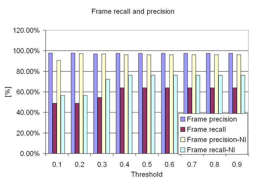
ALBANESE et al.: PPN ACTIVITY DETECTION                                                                                                                          3

                                  Frame 1                      Frame 2                    Frame 3                     Frame 4

                                  Frame 5                      Frame 6                    Frame 7                     Frame 8
Fig. 1.   Example video sequence of a simulated bank attack.

and resource sharing. We refer the reader to David et al                            similarly, occludes(O1 : Object, O2 : Object) returns true if
[21] and Murata [22] for a comprehensive survey on Petri                            and only if O1 occludes O2 in the current frame4 .
nets. Several forms of Petri nets (PN’s) such as Colored                               For the remainder of the discussion, without loss of general-
PN’s, Continuous PN’s, Stochastic timed PN’s, Fuzzy PN’s etc                        ity 5 , we will assume that action symbols are propositional in
have been proposed. Colored PN’s associate a color to each                          nature. The image processing library associates a subset of A
token, hence are useful to model complex systems where each                         with every frame (or block of frames) in the video sequence.
token can potentially have a distinct identity. In Continuous                       Formally, a labeling is a function ℓ : v → 2A , where v is a
PN’s, the markings of places are real numbers and not just                          video sequence and 2A is the power set of A. For example,
integers. Hence, they can be used to model situations where                         consider the labeling process on the video sequence in Figure
the underlying physical processes are continuous in nature.                         1.
Stochastic timed Petri nets [23] associate, to each transition,                        Example 1: Let A = {outsider − present, employee −
a probability distribution which represents the delay between                       present, outsider − absent, employee − absent, outsider −
the enabling and firing of the transition. Fuzzy Petri nets [24]                    insaf ezone, employee − insaf ezone}. The labeling of the
are used to represent fuzzy rules between propositions.                             video sequence in Figure 1 w.r.t. A is given by:
   In real-life situations, vision-based systems have to deal                       ℓ(f rame1) = {outsider − absent, employee − absent}
with ambiguities and inaccuracies in the lower-level detection                      ℓ(f rame2) = {outsider − present, employee − absent}
and tracking systems. Moreover, activities may not unfold                           ℓ(f rame3) = {outsider − present, employee − present}
exactly in the sequence as laid out by the model that represents                    ℓ(f rame4) = {outsider − insaf ezone, employee −
it. The aforementioned versions of Petri nets (continuous,                          insaf ezone}
stochastic, fuzzy) are not well suited to deal with these                           ℓ(f rame5) = {outsider − absent, employee − absent}
situations. The proposed probabilistic Petri net model is well-                     ℓ(f rame6) = {outsider − insaf ezone, employee −
suited to express uncertainty in the state of a token or associate                  insaf ezone}
a probability to a particular unfolding of the PN.                                  ℓ(f rame7) = {outsider − present, employee − present}
                                                                                    ℓ(f rame8) = {outsider − absent, employee − present}
                                                                                    In this example, the presence of the outsider − present
A. Labeling of Video Sequences                                                      label for frame 2 means that an outsider (a person who
                                                                                    is not an employee) is present in that frame. Similarly,
   There has been significant effort in computer vision to                          employee − present in frame 3 means a person whose face
address the problem of detecting various types of elementary                        is recognized as that of an employee is present in frame 3,
events or actions from video data, such as a person entering or                     whereas employee − insaf ezone means an employee is near
leaving a room or unloading a package. Corresponding to the                         the bank safe (on the left-hand side of the image).
set of atomic or primitive actions, we assume the existence
of a finite set A of action symbols. Image understanding
algorithms3 are used to detected these atomic actions. In                           B. Constrained Probabilistic Petri Nets
general, the action symbols can be arbitrary logical predicates                       We define a constrained probabilistic Petri net (PPN) as the
a : Ok → {true, f alse}, where O is the set of objects                              tuple P P N = {P, T, →, F, δ} where
in the video and k is the arity of the action symbol a. To                            1) P and T are finite disjoint sets of places and transitions
provide a few examples used for the TSA dataset, pickup(P :                               respectively i.e. P ∩ T = ∅.
P erson, O : Object) returns the value true if person P has                           2) → is the flow relation between places and transitions,
picked up object O in the current frame and false otherwise;                              i.e., →⊆ (P × T ) ∪ (T × P ).
   3 Although some of the image understanding methods cited in this paper re-         4 According   to the occlusion detection algorithm.
turn a numeric value in the unit interval [0, 1], this can be readily transformed     5 For a finite object domain, we can “flatten” predicates of any arity to the
into a method that returns either “yes” or “no” based on a fixed threshold.         propositional case.
4                                                                                                                               IEEE TRANSACTIONS ON MULTIMEDIA

    3) The preset of a node x ∈ P ∪ T is the set {y|y → x}.                          Skip
                                                                                                            Car
                                                                                                            Enter
                                                                                                                      p1              p3     Person
                                                                                                                                             Enter
                                                                                                                                                       0.1
                                                                                                                                                                  Skip
       This set is denoted by the symbol . x.                                          t2
                                                                                                     0.1
                                                                                                                0.9                              0.9         t4
    4) The postset of a node x ∈ P ∪ T is the set {y|x → y}.                                     Car Stop                  t1    t5                    Person Disappears
       This set is denoted by the symbol x. .                                                                                                          Near Car

    5) F is a function defined over the set of places P , that
                                                                                                                      p2              p4               0.1
       associates to each place x a local probability distribution                    Skip                                                                        Skip
                                                                                                      0.1
       over {t|x → t}. F : x 7−→ fx (t), where x ∈ P and                                    t3
                                                                                                                       0.9             0.9
                                                                                                                                                             t6

       fx (t) is a probability distribution defined over the postset
                                                                                                                      t6          Car Leaves
       of x. For each place x ∈ P in a given PPN, we denote
       by p∗ (x) the maximum product of probabilities over all                                                         p5

       paths from x to a terminal node. We will often abuse
       notation and use F (x, t) to denote fx (t).                       Fig. 2.   Probabilistic Petri net for Car-pickup
    6) δ : T → 2A associates a set of action symbols
       with every transition in the Petri Net. Intuitively, this
       imposes constraints on the transitions in the Petri Net –         the token is removed from p1 and placed in p2 . This leads to
       transitions will only fire when all the action symbols in         a new marking µ2 such that µ2 (p2 ) = 1 and µ2 (p) = 0 for
       the constraint are also encountered in the video sequence         all p 6= p2 . Similarly, when a person enters the parking lot, a
       labeling.                                                         token is placed in p3 and transition t5 fires after the person
    7) ∃x ∈ P s.t. x. = ∅. This means that there exists at least         disappears near the parked car. The token is then removed from
       one terminal node in the Petri net.                               p3 and placed in p4 . Now, with a token in each of the enabling
    8) ∃x ∈ P s.t. . x = ∅. This means that there exists at least        places of transition t6 , it is ready to fire when the associated
       one start node in the Petri net.                                  condition i.e. car leaving the parking lot is satisfied. Once the
                                                                         car leaves, t6 fires and both the tokens are removed and a
                                                                         token placed in the final place p5 . This example illustrates
C. Tokens and Firing of transitions                                      sequencing, concurrency and synchronization.
    The dynamics of a Petri net are represented by means of                 In the above discussion, we have not yet discussed the prob-
‘markings’. For a PPN (P, T, →, F, δ), a marking is a function           abilities labeling some of the place-transition edges. Note that
µ : P → N that assigns a number of tokens to each place                  the postsets of p1 , p2 , p3 , p4 contain multiple transitions. These
in the PPN. For example, µ(p1 ) = 2 means that according                 ‘skip’ transitions are used to explain away deviations from the
to marking µ, there are two tokens in place p1 . For a PPN               base activity pattern – each such deviation is penalized by a
representing an activity, a marking µ represents the current             low probability. For example, after the car enters the scene,
state of completion of that activity. The token is simply an             suppose that instead of stopping in a lot, the car goes around
abstract representation of a partial state.                              in circles. In this case, the skip transition is fired, meaning a
    The execution of a Petri net is controlled by its current            token is taken from p1 and immediately placed back. However,
marking. A transition is said to be enabled if and only if all           the token probability is decreased by the probability labeling
its input places (the preset) have a token. When a transition            the edge to the skip transition.
is enabled, it may fire. When a transition fires, all enabling
tokens are removed and a token is placed in each of the output              All tokens are initially assigned a probability score of 1.
places of the transition (the postset). We will denote by µ0             Probabilities are accumulated by multiplying the token and
the initial marking of a PPN. As transitions fire, the marking           transition probabilities on the edges. When two or more tokens
changes for the places in the preset and postset of the transition       are removed from the net and replaced by a single token –
being fired. A terminal marking is reached whenever one of               for instance when t6 fires – then the net probability for the
the terminal nodes contains at least one token. In the simplest          new token is set to be the product of the probabilities of the
case, all the enabled transitions may fire. However, to model            removed tokens. We will use the final probability of a token in
more complex scenarios we can impose other conditions to                 a terminal node as the probability that the activity is satisfied.
be satisfied before an enabled transition can fire. This set of             Example 3: Figure 3 depicts another constrained PPN mod-
conditions is represented by δ.                                          eling two possible ways in which a successful bank robbery
    Example 2: Consider an example of a car pickup activity              may happen. Uncertainty appears after both the employee and
represented by a probabilistic Petri Net as shown in figure 2.           outsider are inside the zone of the bank safe (at place p5 ).
In this figure, the places are labeled p1 , . . . , p5 and transitions   According to the model, in 60% of the cases both the attacker
t1 , . . . , t6 . We denote by µ0 the initial marking depicted in the    and the employee will enter the safe (visually, this means that
figure in which all places have 0 tokens. In this PN, p1 and             they will disappear from view for a period of time) – this is
p3 are the start nodes and p5 is the terminal node. When a car           modeled starting with p7 , whereas in 35% of the cases, the
enters the scene, a token is placed in place p1 and we have              attacker enters the safe alone (p6 ). In either case, a successful
a new marking µ1 such that µ1 (p1 ) = 1 and µ1 (p) = 0 for               robbery is completed once the outsider leaves the scene (p12 ).
any p 6= p1 . The transition t1 is enabled in this state, but it         Note the use of skip transitions to model possible “noise” in
cannot fire until the condition associated with it is satisfied –        the labeling (i.e. labels that do not correspond to any of the
i.e., when the car stops near a parking slot. When this occurs,          currently enabled transitions) as explained previously.
ALBANESE et al.: PPN ACTIVITY DETECTION 5
Skip-state Skip-state
Skip-state
0.05 0.05
outsider-present outsider-absent αj1
outsider -insafezone ,
employee -insafezone 0.05
pj1 pj1
p1 0.95 p3 p6
0.35 αj2
p0
t2 0.95
p5
t5 pj2 pj2 αk = αj1 ∗ αj2 ∗ . . . ∗ αjn
* employee -present 0.95
outsider -absent outsider -absent
0.6
t4
t1 p2 0.95 p4 pk
pk
p7 p8
t3
0.05 0.05
t6 t7
outsider-insafezone,
Skip-state Skip-state
employee -insafezone t8 αjn
outsider-absent pjn pjn
p11 0.95 p10
t9
(a) (b)
0.05
Skip-state
Fig. 6. Synchronization (a) Before Firing (b) After firing
Fig. 3. Constrained PPN depicting a bank attack dead - dead -
end end
forbidden -action greater _than(current _frame -
t1 t1 last_ trans_frame, 20 )
α2 = α1 ∗ fp1 (t1 )
α1
fp1 (t1 ) p2 fp1 (t1 ) p2
1.00
permitted-action 1.00 less_than_eq(current _frame-
last_trans _frame, 20)
t2 t2
p1 p1
fp1 (t2 ) fp1 (t2 ) p1 0.95 p2 p1 0.95 p2
p3 p3
t1 t1
(a) (b)
(a) (b)
Fig. 4. (a) Before Firing (b) After firing of transition t1
Fig. 7. (a) Forbidden actions (b) Temporal constraints
E. Enhancing PPN expressiveness: Forbidden actions and
D. Rules for token probability computation Temporal durations
In this section, we will describe how PPNs can be used
We denote by αk the value or probability associated with a to model “forbidden actions” – actions which trigger the
token at place pk . When a token is placed in one of the start recognition of a partially completed activity to be nullified
nodes, it is associated with a value of 1 (or some other prior – and constraints on the temporal duration of the activity.
probability for instance, as reported by the low-level vision Forbidden Actions: In several applications, it is important
module). Figure 4 shows how the value associated with a token to be alert to suspicious behavior that should immediately
gets updated as a transition fires. In this figure, transitions t1 trigger an alarm. We show how forbidden actions can be
and t2 are both enabled. fp1 is the local probability distribution modeled in Figure 7(a). This is possible when the set of
associated with the place p1 . If transition t1 fires, then the forbidden actions is mutually exclusive to the set of permitted
value of the token in place p2 becomes α2 = α1 ∗ fp1 (t1 ) actions. Essentially, for each forbidden action fa that may
as shown in figure 4. The probability computation rules for occur in a given state, we add a transition with probability
synchronization and concurrency are illustrated in figures 5 1 conditioned on fa to a place that is a dead-end (i.e., no
and 6 respectively. terminal marking can be reached from it).
Temporal Duration: Oftentimes activities are constrained
not just by a simple sequencing of action primitives, but also
by the duration of each action primitive in the sequence. In
αk1 = αj general, we may associate a probability distribution over the
pk1 pk1 ‘dwell’ time to each place in the Petri net. We have used a
αk2 = αj simplified version where we constrain the dwell time to be
αj
pk2 pk2 upper and lower bounded. We have built a few macros that
handle frame computation. For instance, current f rame is
pj pj
the number of the current frame, whereas last trans f rame
is the number of the last frame at which a transition was fired
αkn = αj for the current activity. Intuitively, Figure 7(b) imposes the
pkn pkn condition that the transition t1 fire within twenty frames of
the last transition that was fired. If this does not occur, then
(a) (b) we again transition to a dead-end, as in the case of forbidden
actions.
Fig. 5. Concurrency (a) Before Firing (b) After firing
6                                                                                                                    IEEE TRANSACTIONS ON MULTIMEDIA

F. Activity recognition                                                         variant of PPN-MPS can be used to naively solve the PPN-
    We now define a ‘PPN trace’ and what it means for a video                   MPA problem in a naive fashion – we call this the naivePPN-
sequence to satisfy a given PPN and provide a method for                        MPA. Finally, we provide a greatly improved version of the
computing the probability with which an activity is satisfied.                  PPN-MPA algorithm.
    Definition 1 (PPN trace): A trace for a PPN (P, T, →                            The PPN-MPS algorithm (Algorithm 1) is based on the pro-
, F, δ) with initial marking µ0 is a sequence of transitions                    cess of simulating the constrained PPN forward. The algorithm
ht1 , . . . , tk i ⊆ T such that:                                               uses a separate structure to store tuples of the form hµ, p, fs i,
                                                                                where µ is a valid marking, p is the probability of the partial
  (i) t1 is enabled in marking µ0 .
                                                                                trace that leads to the marking µ and fs is the frame when the
 (ii) Firing t1 , . . . , tk in that order reaches a terminal marking.
                                                                                first transition in that trace was fired. The PPN-MPS algorithm
For each i ∈ [1, k], let pi = Π{x∈P |x→t} F (x, t). We say the                  takes advantage of the fact that we only need to return minimal
trace ht1 , . . . , tk i has probability p = Πi∈[1,k] pi . Let pmax             subsequences and not the entire PPN traces that lead to them,
be the maximum probability of any trace for (P, T, →, F, δ).                    hence using the last marking as a state variable is sufficient
                                                        p
Then ht1 , . . . , tk i has relative probability pmax      .                    for our purposes.
    Example 4: Consider                   the   PPN    in    Figure        3.       The algorithm starts by adding hµ0 , 1, 0i to the store S
ht1 , t3 , t2 , t4 , t5 , t8 , t9 i is a trace with probability .2708           (line 1). This means we start with the initial marking (µ0 ),
and relative probability .5833. ht1 , t2 , t3 , t4 , t6 , t7 , t8 , t9 i is a   with the probability equal to 1. The value 0 for the start
trace with probability .4642 and a relative probability of 1.                   frame means the first transition has not yet fired. Whenever
    Definition 2 (Activity satisfaction): Let P = (P, T, →                      the first transition fires and the start frame is 0, the current
, F, δ) be a PPN, let v be a video sequence and let ℓ be the                    frame is chosen as a start for this candidate subsequence
labeling of v. We say ℓ satisfies P with relative probability                   (lines 8–9). The algorithm iterates through the video frames6 ,
p ∈ [0, 1] iff there exists a trace ht1 , . . . , tk i for P such that:         and at each iteration analyzes the current candidates stored in
  (i) There exist frames f1 ≤ . . . ≤ fk such that ∀i ∈ [1, k],                 S. Any transitions t enabled in the current marking from S
       δ(ti ) ⊆ ℓ(fi ) AND                                                      that have the conditions δ(t) satisfied are fired. The algorithm
 (ii) The relative probability of ht1 , . . . , tk i is equal to p.             generates a new marking, and with it a new candidate partial
    We will refer to a video sequence v satisfying an activity                  subsequence (line 7). If the new probability value p′ (lines 13 –
definition, as an equivalent way of saying the labeling of v                    14) is still above the threshold (line 15) and can remain above
satisfies the activity. For reasons of simplicity, if ℓ is the                  the threshold on the best path to a terminal marking (line 16),
labeling of v and v ′ ⊆ v is a subsequence of v, we will also                   the new state is added to the store S. This first pruning does
use ℓ to refer to the restriction of ℓ to v ′ .                                 away with any states that will result in low probabilities. Note
    Example 5: Consider the video sequence in Figure 1 with                     that we have not yet removed the old state from the store –
the labeling in Example 1, and the activity PPN in Fig-                         nor should we at this time, since we also need to fire any skip
ure 3. The labeling in Example 1 satisfies the PPN with                         transitions that are available. This is done for any enabled skip
relative probability 1 since the conditions for the trace                       transition on line 26. At this point we also prune away any
ht1 , t2 , t3 , t4 , t6 , t7 , t8 , t9 i are subsets of the labeling for        states in S that have no possibility of remaining above the
frames 1 – 8.                                                                   threshold as we reach a terminal marking (line 27).
    We now define the two types of queries we are interested                        Example 6: We illustrate the working of PPN-MPS on the
in answering.                                                                   PPN in Figure 3, the labeling in Example 1 and pt = 0.5.
    The Threshold Activity Query Problem (PPN-MPS) can                          Initially, S = hµ0 , 1, 0i. We will denote by µi the marking
be formulated as following: given a constrained PPN, a video                    obtained after firing ti in Figure 3. At frame 1, since transition
sequence v and a probability threshold pt , find the minimal                    t1 has no precondition, it will fire and we will have one new
subsequences of v that satisfy the PPN with probability at                      element in S (along with the existing initial state) – hµ1 , 1, 0i.
least pt . Intuitively, such queries are of interest for identifying            Note that the starting frame is still set to 0 – this is done so that
specific portions of the video sequence in which a given                        the start of the subsequence is marked only when a labeling
activity occurs.                                                                condition is satisfied. At frame 2, transition t2 fires and we
    The Activity Recognition Query Problem (PPN-MPA) is                         add hµ2 , .95, 2i to S. At this point, transition t3 is enabled but
formulated as follows: Given a set of activities {P1 , . . . , Pn }             cannot fire because its condition employee − present is not
and a video sequence v, determine which activity (or set of                     satisfied. Hence a skip transition fires, but that generates a state
activities) is satisfied by the labeling of v with maximum                      with probability .05, which is under the threshold and hence
probability. Intuitively, such queries are useful in scenarios in               thrown away immediately. We will ignore the firing of skip
which video sequences are processed semi-automatically and                      transitions for the rest of the example, as they are immediately
we are interested in finding which activity occurs in a given                   pruned away due to the low probabilities generated. Transition
sequence.                                                                       t3 does fire at frame 3 and adds hµ3 , .9025, 1i to S. Transition
                                                                                t4 is now enabled and its conditions satisfied at frame 4, hence
    III. A LGORITHMS      FOR   T HRESHOLD ACTIVITY Q UERIES                    it is fired and a new state hµ4 , .8145, 1i is generated. At frame

  We start this section by presenting an efficient algorithm                      6 In our implementation, we group frames with identical labeling into blocks
for the PPN-MPS problem. We then show how an iterative                          and iterate over blocks instead which leads to enhanced efficiency.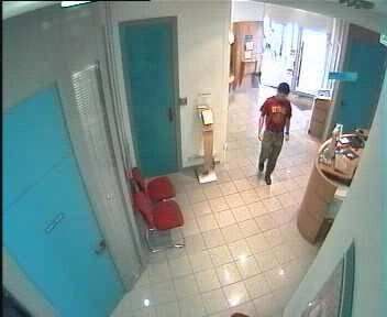
ALBANESE et al.: PPN ACTIVITY DETECTION 7
Algorithm 1 Threshold Activity Queries (PPN-MPS) p0
probability of the trace. Then p · pk ≥ max p
≥ pt , (condition
Input: P = (P, T , →, F, δ), initial configuration µ0 , video sequence labeling ℓ, probability threshold pt
Output: Set of minimal subsequences that satisfy P with relative probability above pt on line 15 holds). Also, for all x ∈ P that receive a token as tk
p0
1: S ← {hµ0 , 1, 0i}
2: R ← ∅ fires, p · pk · p∗ (x) ≥ max p
≥ pt (condition on line 16 holds);
3: maxp ← the maximum probability for any trace of P P N line 17 therefore executes and the new marking µk (including
4: for all f frame in video sequence do
5: for all hµ, p, fs i ∈ S do the effects of firing tk ) is added to S (induction step). We
6: for all t ∈ T enabled in µ s.t. δ(t) ⊆ ℓ(f ) do
7: µ′ ← fire transition t for marking µ showed by induction that a trace of probability greater than
8: if fs = 0 and δ(t) 6= ∅ then
9: f′ ← f or equal to pt corresponding to a subsequence of v0 has been
10: else
executed.
11: f ′ ← fs
12: end if
∗ Theorem 2 (PPN-MPS complexity): Let P = (P, T, →
13: p ← Π{x∈P |x→t} F (x, t)
14: p′ ← p · p∗ , F, δ) be a PPN with initial configuration µ0 , such that the
15: if p′ ≥ pt · maxp then
16: if ∀x ∈ P s.t. µ(x) < µ′ (x) it holds that p′ · p∗ (x) ≥ pt · maxp then number of tokens in the network at any marking is bounded
17: S ← S ∪ {hµ′ , p′ , f ′ i}
18: end if
by a constant k 8 . Let v be a video sequence and ℓ its labeling.
19:
20:
end if
if µ′ is a terminal configuration then
Then PPN-MPS runs in time O(|v| · |T | · |P |k ).
21: S ← S − {hµ′ , p′ , f ′ i} Proof. We will first look at how many possible markings
22: R ← R ∪ {[fs , f ]}
23: end if there are if the PPN is bounded by k. If we denote the number
24: end for
25: for all t ∈ T enabled do of possible markings for a PPN with n nodes which is bounded
26: Fire skip transitions if no other transitions fired and update hµ, p, fs i
27: Prune hµ, p, fs i ∈ S s.t. ∀x ∈ P s.t. µ(x) > 0, p · p∗ (x) < pt · maxp {Pruning by k by xn,k , then by fixing one token (n possibilities), we
always keeps hµ0 , 1, 0i in S}
28: end for have that xn,k = n·xn,k−1 . This leads to xn,k = nk−1 ∗xn,1 =
29:
30:
end for
end for nk ∗xn,0 = nk . The algorithm process each frame in the video
31: Eliminate non-minimal subsequences in R
32: return R (line 4), at each iteration looking at every element of S (line
5); however, there are at most a constant number of elements
in S for each marking, therefore the size of S is O(|P |k ). For
5, transition t6 is satisfied (and t5 is not), hence it is fired and every element in S, we look at at most |T | transactions enabled
the state becomes hµ5 , .4880, 1i. Finally, t7 , t8 , t9 are fired at for that marking, hence the complexity result. We normally
frames 6, 7, 8 and bring the final state to µ8 , .4642, 1i, leading expect that in regular activity definitions, the degree k of the
to a relative probability of 1 (we remind the reader that the polynomial is small; also, for a fixed activity definition, the
elements of S hold the absolute probability). algorithm is linear in the size of the video.
The following theorem states that the PPN-MPS algorithm We should point out that the probabilities in the PPN already
returns the correct result. enforce a bound on the number of tokens in the network.
Theorem 1 (PPN-MPS correctness): Let P = (P, T, → Assume that there are no transactions with a probability of
, F, δ) be a PPN with initial configuration µ0 , let v be a 1 (for instance, by adding skip transitions at every place). Let
video sequence and ℓ its labeling, and let pt ∈ [0, 1] be a c be the upper bound of the probabilities in P. New tokens are
probability threshold. Then for any subsequence v ′ ⊆ v that generated as a result of transitions with a postset of cardinality
satisfies P with probability greater than or equal to pt , one of strictly greater than 1 – one can generate at most |P − 2| new
the following holds: tokens on each such transition. Furthermore, for a threshold
(i) v ′ is returned by PPN-MPS OR pt , each token can be used to fire at most log pt
log c transitions
(ii) ∃v ′′ ⊆ v that is returned by PPN-MPS such that v ′′ ⊆ v ′ . before the probability is lowerP than pt . Assuming the initial
Proof Let v0 ⊆ v be a subsequence of v that satisfies the number of tokens is |µ0 | = µ0 (x), this means we can
x∈P
activity definition, but is not returned by PPN-MPS. If v0 has a log pt
have at most |µ0 | · |P − 2| log c tokens in the network.
subsequence returned by PPN-MPS, we are done. Otherwise,
Handling Multiples Instances: Note that PPN-MPS
since v0 satisfies the activity definition, according to Definition
already handles a certain degree of parallelism in the activities
2, there exists a trace ht1 , . . . , tn i and corresponding frames
occurring in the video. This is a direct consequence of the
(in v0 ) f1 ≤ . . . ≤ fk such that ∀i ∈ [1, k], δ(ti ) ⊆ ℓ(fi ).
fact that hµ0 , 1, 0i is always a member of S, hence a new
We will show by induction that the algorithm will fire all
activity could be started at every frame. However, PPN-
transitions (ti )i∈[1,n] . Since hµ0 , 1, 0i always remains in S,
MPS does not directly handle the case in which multiple
and t1 is executable from µ0 and δ(t1 ) ⊆ ℓ(f1 ), then t1
actions that start an activity (i.e., enable a transition from
must be fired on line 7 and f1 becomes the current frame
hµ0 , 1, 0i) occur in the same frame. In our implementation, we
(initial condition). Assume that all transitions up to (ti )i∈[1,k]
handled this case by duplicating the PPN for each action of a
have been fired; we want to show that tk must fire next.
frame that can potentially start a new activity. The maximum
Assume that the new state in S induced by the firing of tk−1
number of such actions per frame is maxf ∈v (|ℓ(f )|). Hence,
is sk−1 = hµk−1 , pk−1 , f1 i such that tk is enabled in µk−1 .
taking the complexity of the scene into account, the worst-
Since (ti )i∈[1,k] is a trace, then when frame fk is analyzed,
case complexity becomes O(maxf ∈v (|ℓ(f )|) · |v| · |T | · |P |k ).
there must exist a state sk = hµk−1 , p, f1 i ∈ S (if multiple
However, in our two datasets we only needed duplication in
such states exist, then we choose the one with the highest
under 1% of the frames, and maxf ∈v (|ℓ(f )|) ≤ 3 in all cases.
probability)7. Let pk be the probability of firing tk (which is
enabled and has δ(tk ) satisfied on line 6) and let p0 be the 8 This is called a bounded PPN – i.e., one that does not generate an infinite
number of tokens. We will see that the probabilities in the PPN may enforce
7p may be different than pk by firing skip transitions. a variant of this rule.
8 IEEE TRANSACTIONS ON MULTIMEDIA
IV. A LGORITHMS FOR ACTIVITY R ECOGNITION the activity definitions in R are satisfied by the video with
Let us now consider the PPN-MPA problem. Let maximal probability.
{P1 , . . . , Pn } be a given set of activity definitions. If we Theorem 3 (PPN-MPA correctness): Let {(Pi , Ti , →i
assume that there is only one activity Pl which satisfies the , Fi , δi )}i∈[1,m] be a set of PPNs, let v be a video sequence
video sequence v with maximal probability, a simple binary and ℓ its labeling. Let P1 , . . . , Pk be the activity definitions
search iterative method – which we shall call naivePPN-MPA returned by PPN-MPA. Then the following hold:
– can employ PPN-MPS to find the answer: (i) ∀i ∈ [1, k], let pi be the relative probability with which
1) Begin with a very high threshold pt . ℓ satisfies Pi . Then p1 = . . . = pk .
2) Run PPN-MPS for all activities in {P1 , . . . , Pn } and (ii) ∀P ′ ∈ {(Pi , Ti , →i , Fi , δi )}i∈[1,m] − {P1 , . . . , Pk }, ℓ
threshold pt . does not satisfy P ′ with relative probability greater than
3) If more than one activity definition has a non-empty or equal to p1 = . . . = pk .
result from PPN-MPS, then increase the threshold by Proof. The proof of correctness for PPN-MPS shows that
1−pt the algorithm does not “miss” transitions, but ignores only
2 and go to step 2.
4) If no activity has a non-empty result from PPN-MPS, those that cannot end up above the threshold. In this case,
decrease the threshold by p2t and go to step 2. the threshold is the variable maxp , which means the only
5) If only one activity Pl has a non-empty result from PPN- transitions being ignored are those for which there is already
MPS, return Pl . a “better” activity (satisfied with the probability maxp ) in R;
Clearly, this method can be improved to account for the this is sufficient for condition (ii). Condition (i) is satisfied
case in which multiple activity definitions are satisfied by the by the fact that maxp always increases (lines 19–24) and all
video sequence with the same probability. Even under these elements in R must be satisfied with the same probability (line
conditions, the algorithm requires multiple passes through the 22).
video (for each run of PPN-MPS) until a delimiter threshold Theorem 4 (PPN-MPA complexity): Let {(Pi , Ti , →i
is found. We will now present a much more efficient method , Fi , δi )}i∈[1,m] be a set of PPNs, let v be a video sequence
– the PPN-MPA algorithm. and ℓ its labeling. PPN-MPA runs in time O(m·|v|·|T |·|P |k ).
Proof. The same reasoning as for PPN-MPS applies here
Algorithm 2 Activity recognition queries (PPN-MPA) as well, with the addition of the factor m which accounts for
Input: Set of PPNs {(Pi , Ti , →i , Fi , δi )}i∈[1,m] , initial set of configurations µ0
i , video sequence labeling
the size of S when we analyze m different activities.
ℓ
Output: Set of PPNs that is satisfied by ℓ with maximal probability Similarly to PPN-MPS, PPN-MPA will clone the PPNs each
1: for all {Pi , Ti , →i , Fi } do time multiple actions in a single frame can potentially start a
2: S ← S ∪ {hµ0 i , 1i}
3: end for new activity. Taking into account the maximum number of
4: maxp ← 0
5: R ← ∅ such actions would yield a complexity of O(maxf ∈v (|ℓ(f )|) ·
6: for all f frame in video sequence do
7: for all hµ, pi ∈ S do m · |v| · |T | · |P |k ), however in practice we only needed to
8: for all t ∈ T enabled in µ s.t. δ(t) ⊆ ℓ(f ) do
9: µ′ ← fire transition t for marking µ clone the PPNs very rarely.
10: p∗ ← Π{x∈P |x→t} F (x, t)
11: p′ ← p · p∗
12: if p′ ≥ pt · maxp then
13: if ∀x ∈ P s.t. µ′ (x) > 0, p′ · p∗ (x) ≥ pt · maxp then
V. S YSTEM I MPLEMENTATION
14: S ← S ∪ {hµ′ , f ′ i}
15: end if Our PPN-MPS, naivePPN-MPA and PPN-MPA algorithms
16: end if
17: if µ′ is a terminal configuration then were implemented in Java. In addition, our image processing
18: S ← S − {hµ′ , p′ i}
19: if p > maxp then library is based on the People Tracker framework of [25] with
20: R ← { activity definition corresponding to µ′ }
21: maxp ← p
several modifications outlined in this section.
22: else if p = maxp then The People Tracker9 [25], [26] uses object detection and
23: R ← R ∪ { activity definition corresponding to µ′ }
24: end if motion algorithms to track persons, groups of persons, vehicles
25: end if
26: end for and other objects in a given sequence of images. From a
27: for all t ∈ T enabled do
28: Fire skip transitions and update hµ, pi functional point of view, the framework consists of four
29: Prune hµ, pi ∈ S s.t. ∀x ∈ P s.t. µ(x) > 0, p · p∗ (x) < pt · maxp
30: end for
components:
31: end for
32: end for 1) The Motion Detector subtracts the background from the
33: return R
current image and thresholds the resulting difference
image to obtain moving objects (“blobs”).
PPN-MPA (Algorithm 2) uses the same storage structure as 2) The Region Tracker tracks all blobs identified in the pre-
PPN-MPS. However, this time we are no longer interested
vious step by a frame-by-frame matching algorithm. The
in the start and end frames of the subsequences matching
next position of a blob is predicted using a first-order
one of the activity definitions. Instead, we maintain a global
motion model and then matched against the positions of
maximum relative probability (maxp ) with which the video
the blobs in the new frame.
satisfies any of the activities in {Pi , Ti , →i , Fi , δi }. maxp 3) The Head Detector is used to identify blobs correspond-
is updated any time a better relative probability is found
ing to people by creating a vertical projection histogram
(lines 19–21); R maintains a list of the activity definitions
that have been satisfied with the relative probability maxp . 9 Freely available under a public GPL license at http://www.siebel-
At the return statement on line 33, we are guaranteed that research.de.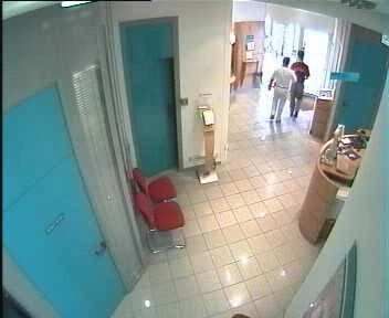
ALBANESE et al.: PPN ACTIVITY DETECTION 9
of the upper part of every tracked region. This is based model, as well as sets of activity definitions for each video
on the algorithms of Haritaoglu et al. [27]. and were asked to mark the starting and ending frame of each
4) The Active Shape Tracker uses B-spline 2D shape mod- activity they encountered. An average over the four reviewers
els to resolve the type of a tracked region to a person, was then considered as our ground truth dataset for the
group of persons, vehicle, package, etc. purpose of computing precision and recall. We compared the
In addition to these, the following extensions were made: subvideos provided by the reviewers (note that probabilities
1) Shadows reduced the accuracy of detecting object splits were completely hidden from the users.) with those returned
and merges. To take care of this, we implemented the by our algorithms above a given probability threshold value.
algorithm of [28] for detection of moving shadows. All experiments were performed on a Pentium 4 2.8 GHz
2) We implemented the face recognition algorithm of [29]. machine with 1 GB of RAM running SuSE Linux 9.3. The
The algorithm detects faces in a frame using a wavelet labeling data generated by the low-level vision methods was
transform based approach and then compares features stored in a MySQL database. The labeling was compressed
of detected faces and faces stored in the database. We for blocks of frames, as neighboring frames often tend to
chose this particular face recognition algorithm because have identical labeling. Running times include disk I/O for
of its speed and good accuracy. accessing the labeling database, but not the time taken to
3) To accurately answer queries of type: “Is object O in generate the labeling.
frame f ?”, one needs to perform occlusion analysis. We
implemented the occlusion detection algorithm of [30] A. Experimental evaluation for the Bank dataset
for this task. For the Bank dataset, we defined a set of 5 distinct activities
Based on the output of the above framework and the and constructed the associated PPNs. They are:
aforementioned extensions, we implemented a number of low- (a1) Regular customer-bank employee interaction.
level predicates to answer simple queries such as: (a2) Outsider enters the safe.
1) Is object O present in frame f (in a particular zone (a3) A bank robbery attempt – the suspected assailant does
Z)? This is accomplished through the object matching not make a getaway.
algorithm in the Region Tracker module. (a4) A successful bank robbery similar to the example in
2) Is object Oi occluding Oj in frame f ? Figure 3.
3) Are objects Oi and Oj splitting/merging in frame f ? (a5) An employee accessing the safe on behalf of a customer.
4) What is the type of object Oi (person, vehicle, group of For the PPN-MPA experiments, we grouped these into dif-
persons, etc.) in frame fi ? ferent sets of activities as: S1 = {a5}, S2 = {a3, a5},
5) Is object O identical to the person P from the database S3 = {a3, a4, a5} and S4 = {a2, a3, a4, a5}.
? For the PPN-MPS algorithm, we observed empirically that
All the above queries are typically answered with a degree in the majority of cases, at most one instance of the activity
of confidence reported as a probability by the underlying occurs at any given time. For instance, it is highly unlikely
low-level module. Finally, we have combined these low-level that we have two bank attacks (a3, a4) interleaved in the same
queries into sequences in order to generate the higher-level video sequence; although we might have a number of regular
labeling our algorithms take as input. customer operations (a1), we assumed that the special events
we are interested in monitoring are generally rare. We took
VI. E XPERIMENTAL R ESULTS this into account by developing two different versions of the
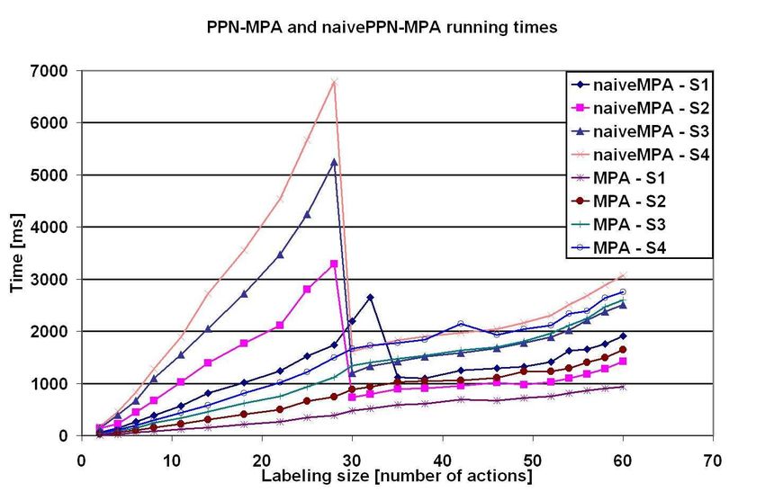
Our experiments were performed on two datasets. The first algorithm. The first is the one depicted in Section III; the
dataset (Bank) consists of 7 videos of 15–20 seconds in length, second version optimizes the algorithm by assuming there can
some depicting staged bank attacks and some depicting day- be no interleaving of activities in a video; we will denote
to-day bank operations. The dataset has been documented in the latter with the suffix NI (no interleaving). This approach
[20]. Figure 1 contains a few frames from a video sequence generally leads to an improvement in running time, at the
depicting a staged bank attack. Figure 8(top) contains a expense of precision.
few frames from a video sequence depicting regular bank Running Time Analysis: In our first set of experiments,
operations. The second dataset consists of approximately 118 we measured the running times of PPN-MPS, naivePPN-MPA
minutes of TSA tarmac footage and contains activities such and PPN-MPA for the five activity definitions described above
as plane take-off and landing, passenger transfer to/from the while varying the size of the labeling (the number of action
terminal, baggage loading and unloading, refueling and other symbols in the labeling10 ). The running times are shown in
airport maintenance. Figure 9. As expected, the non-interleaving (NI) version of
We compared the precision and recall of our algorithms PPN-MPS is more efficient than its counterpart. naivePPN-
against the ground truth provided by human reviewers MPA exhibits a seemingly strange behavior – running time
as follows. Four human reviewers analyzed the videos in increases almost exponentially with labeling size, only to drop
the datasets. The reviewers were provided with VirtualDub suddenly at a labeling size of 30. On further analysis of the
(http://www.virtualdub.org), which allowed them to watch the results, we discovered that at this labeling size the activity
video in real time, as well as browse through it frame by 10 We remind the reader that the videos are 15-20 second long and that
frame. They received detailed explanations on the activity labeling has been compressed from frame to block level.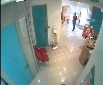
10                                                                                                                 IEEE TRANSACTIONS ON MULTIMEDIA

                           Frame 1 (Bank)             Frame 2 (Bank)            Frame 3 (Bank)             Frame 4 (Bank)

                            Frame 1 (TSA)             Frame 2 (TSA)             Frame 3 (TSA)              Frame 4 (TSA)
Fig. 8.   (top) Example video sequence of regular customer interaction at a bank; (bottom) Sample frames from the TSA dataset.

                                                                                                                 TABLE I
definitions first begin to be satisfied by the labeling. When
                                                                                      M EASURE OF OVERLAP OF SEQUENCES RETURNED BY HUMAN
no activity definition is satisfied, naivePPN-MPA performs
                                                                                   REVIEWERS AND BY THE      PPN-MPS ALGORITHM FOR pt = .7. A
many iterations in order to decrease the threshold close to 0.
                                                                                 MEASURE OF      1 INDICATES PERFECT OVERLAP AND 0 INDICATES NO
Somewhat surprisingly, it is comparable in terms of running
                                                                                                                 OVERLAP.
time with PPN-MPA when the activity is satisfied by at least
one subsequence.                                                                Video      Reviewer 1        Reviewer 2          Reviewer 3       Reviewer 4
                                                                                         |H∩A|     |H∩A|   |H∩A|     |H∩A|   |H∩A|      |H∩A|   |H∩A|    |H∩A|
   Accuracy: In the second set of experiments, we measured                                |H|        |A|    |H|        |A|    |H|         |A|    |H|       |A|
                                                                                  1      .82      1        .83      1        .84       1        .93     1
the precision and recall of PPN-MPS, naivePPN-MPA and                             2      .36      1        .37      1        .38       1        .41     1
PPN-MPA w.r.t. the human reviewers. In the paper describing                       3      .74      1        .83      .93      .67       .97      .72     1
                                                                                  4      .75      1        .78      1        .76       1        .94     .96
the dataset, Vu et al. [20] only provide figures for recall                       5      .56      .99      .58      .98      .58       1        1       .74
between 80% and 100% (depending on the camera angle),
without further details. In this case, the minimality condition
used by the PPN-MPS algorithm poses an interesting problem
– we found that in almost all cases, humans will choose a                     to appear in the answer. The monotonic behavior pattern
sequence which is a superset of the minimal subsequence                       stops when the threshold becomes high enough (.45 in this
for an activity. In order to have a better understanding of                   case). Furthermore, we see that the non-interleaving version
true precision and recall, we compute two sets of measures:                   of the algorithm has a slightly higher recall than the standard
recall and precision at the frame level (Rf and Pf ) and                      version. We observed that human annotators usually focus on
recall and precision at the event (or activity) level (Re and                 detecting one activity at a time and very seldom consider
Pe ). Assume that both the human reviewer and the algorithm                   two or more activities that occur in parallel. Hence, the NI
return a subsequence corresponding to an activity. We will                    version of the algorithm is informally “closer” to how the
denote the subsequence returned by the algorithm A and                        reviewers operate. With respect to the PPN-MPA algorithm,
the one returned by a human reviewer H. Precision/recall                      we see a very good match in terms of the activities returned
measures at the frame level11 are defined as: Pf = |H∩A|  |A|
                                                                              by the human annotators and the ones returned by PPN-MPA
                                                                              for the S4 = {a2, a3, a4, a5} – the most complete dataset.
and Rf = |H∩A|   |H| . However, we can relax this condition                   Poorer performance on the other activity sets is explained
by stating that any subsequence returned by the algorithm
                                                                              by the limitation in the possible choices of the algorithm.
that intersects a subsequence returned by a human reviewer
                                                                              PPN-MPA could only choose activities from a given set,
should be counted as correct. Let the set of sequences returned
                                                                              sometimes missing some results. For instance, if a successful
by the algorithms be {Ai }i∈[1,m] and the set of sequences
                                                                              bank robbery occurs in the video sequence, PPN-MPA cannot
returned by the human annotators be {Hj }j∈[1,n] . Then we
                                 |{Ai |∃Hj s.t. Ai ∩Hj 6=∅}|                  return it from the choices in S2 = {a3, a5}, and thus returns
can write precision as Pe =                  m               and recall       the closest possible match. Lastly, event precision was always
          |{Ai |∃Hj s.t. Ai ∩Hj 6=∅}|
as Re =                n              .                                       100% for PPN-MPS, meaning the algorithm did not yield any
   Figure 10(a) shows the frame precision and recall for the                  false positives. Recall was greater than 90% for the entire
two versions of the PPN-MPS algorithm. We notice that                         dataset for both PPN-MPS and PPN-MPS-NI.
precision is always very high and generally constant, while
                                                                                 Temporal Overlap with Groundtruth: Since precision
recall has a rather surprising variation pattern – namely, recall
                                                                              and recall at the event level was very high, we investigated
is monotonic with the threshold. The explanation for the ap-
                                                                              to what extent the sequences returned by the reviewers and
parently anomalous behavior comes from the fact that for low
                                                                              by PPN-MPS actually overlap. To see why this is relevant,
thresholds, the number of candidate subsequences is relatively
                                                                              consider an 8 frame-video such as the one in Figure 8. Assume
high, hence the minimality condition causes fewer frames
                                                                              that for activity (a5), PPN-MPS returns the subsequence from
  11 Only with respect to one subsequence, but easily extensible to many      frame 1 to frame 4, whereas the human reviewer returns the
subsequences                                                                  subsequence between frames 4 and 8. The event precision and
You can also read