Cash to Spend: IPO Wealth and House Prices - UCLA ...
←
→
Page content transcription
If your browser does not render page correctly, please read the page content below
Cash to Spend: IPO Wealth and House Prices∗
                Barney Hartman-Glaser†                    Mark Thibodeau‡                 Jiro Yoshida§
                                                 November 30, 2018

                                                        Abstract

      This study empirically demonstrates the positive impact of initial public offerings (IPOs) on local housing
      prices in California from 1993 through 2017. In the spirit of the difference-in-difference approach, we test
      whether hedonic price indexes increase after IPO events more for the areas around IPO firm headquarters.
      We use the IPO events of public filing, issuing, and lockup expiration to distinguish changes in the
      shareholders’ expected wealth, assessed wealth, and immediately available wealth, respectively. HPIs
      increase more within 10 miles of IPO headquarters than in the surrounding area by 1.0% after filing and
      0.8% after issuing but approximately zero after lock-up expiration. This result suggests that original
      shareholders change their housing demand when their wealth changes but not when liquidity constraint
      is relaxed. The impact is larger when the wealth increase by IPO is larger; e.g., higher offer price, larger
      IPO proceeds, and larger share underpricing at filing. The impact is also larger for younger and smaller
      firms.

      JEL Classifications: L26, M12, J33, R21
      Keywords: Initial Public Offering, Housing Value, Hedonic Regression, Wealth Effect, Liquidity Con-
      straint, Executive Compensation

   ∗ We thank seminar participants at the University of Tokyo, Hitotsubashi University, Gakushuin University, and Penn State

for their valuable comments and suggestions. We also thank the financial support by UCLA Ziman Center for Real Estate and
Penn State Institute for Real Estate Studies.
   † UCLA, bhglaser@anderson.ucla.edu
   ‡ Pennsylvania State University, mthibodeau@psu.edu
   § The Pennsylvania State University, jiro@psu.edu, 368 Business Bldg., University Park, PA 16802.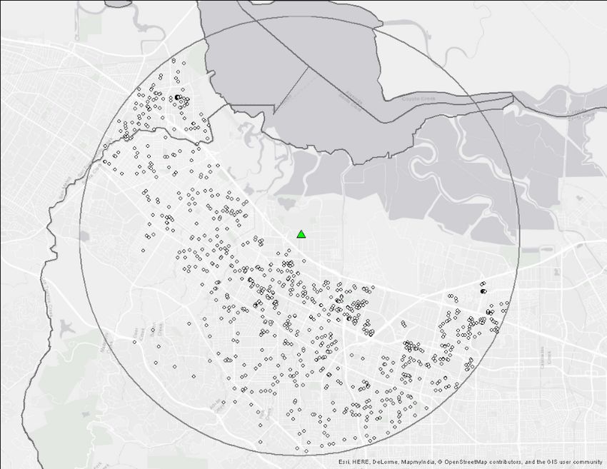
1     Introduction

    An initial public offering (IPO) rewards the founders, angel investors, venture capitalists, and key em-

ployees with stock options (henceforth original shareholders). For example, PrivCo reported that twitter’s

IPO created 1,600 millionaires.1 As a result, original shareholders may experience significant changes in their

wealth and liquidity around an IPO that can lead to changes in their consumption. In particular, demand

may increase for housing and services that impacts the local housing market.

    In California, where start-up companies cluster (Figure 1), a positive correlation is observed between the

number of IPOs and house prices (Figure 2). Although this positive correlation is sometimes interpreted as a

causal effect of the wealth created by a cluster of start-up companies, causality is not immediately obvious.2

Furthermore, if a wealth change is anticipated, the original shareholders would change their consumption and

tenure choices well before an IPO (Friedman, 1957). Thus, for an IPO to affect housing demand, there must

be either unexpected wealth changes or obstacles to consumption smoothing such as liquidity constraints.

Moreover, if IPOs cause the house price appreciation, they may create a negative side-effect on economic

agglomeration through an increase in the cost of living and business (Cornaggia et al., 2017).3

    In this study, we ask two questions. First, do IPOs influence local housing markets? The positive

correlation between IPOs and house prices can be a coincidence or can be generated by confounding factors

such as high amenities and housing supply constraints. We attempt to isolate the causal effect of IPOs on

housing prices. Second, if IPOs influence housing markets, when and how do they influence? Most IPOs have

three sequential events: IPO filing, share issuing, and the expiration of a lock-up period. These sequential

stages provide a unique setting for decomposing a shock to shareholder wealth into an update of the expected

future wealth at the time of an IPO filing, an update of the assessed wealth based on the market share price

at the time of issuance, and the relaxed liquidity constraint at the time of lockup expiration event. The

liquidity constraint can play an important role in housing tenure choice when mortgage financing requires

a significant amount of cash (e.g., Artle and Varaiya, 1978; Schwab, 1982; Slemrod, 1982; Henderson and

Ioannides, 1983; Brueckner, 1986).

    We combine data for IPOs and residential property transactions in California from 1993 through 2017.

To control for the housing heterogeneity, we construct hedonic constant-quality home price indexes (HPIs)
   1 PrivCo    does market research of private firms and reported on twitter’s IPO: http://www.privco.com/
the-twitter-mafia-and-yesterdays-big-irs-payday.
   2 New York Times, February 20, 2017, “With Snap’s I.P.O., Los Angeles Prepares to Embrace New Tech Mil-

lionaires,” (https://www.nytimes.com/2017/02/20/technology/snap-ipo-los-angeles-real-estate.html); and Zillow Blog,
“Millionaire’s Row: How Did Facebook’s IPO Affect Silicon Valley Real Estate?”               (https://www.zillow.com/blog/
millionaires-row-how-did-facebooks-ipo-affect-silicon-valley-real-estate-86027/)
   3 See also San Francisco Business Times, August 16, 2017, “Why 83 percent of Bay Area renters say they plan to leave (https:

//www.bizjournals.com/sanfrancisco/news/2017/08/16/why-83-percent-of-bay-area-renters-say-they-plan.html) and
The Economist, August 30, 2018, “Why startups are leaving Silicon Valley” (https://www.economist.com/leaders/2018/
08/30/why-startups-are-leaving-silicon-valley)

                                                              1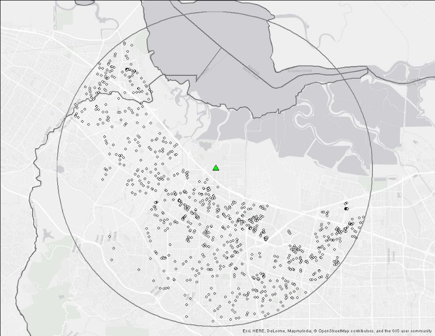
for areas of different proximities to the headquarters of each IPO firm. A monthly HPI is constructed for

each IPO event by using the event date as the base date. Using the event-specific HPIs, we exploit both

the spatial difference in proximity to IPO firms and the discontinuity in time around IPO events. In this

difference-in-differences strategy, the treatment group is housing transactions occurring near the IPO-firm’s

headquarters and a treatment is an IPO event.

    We utilizes original shareholders’ housing preferences for the proximity to the firm’s headquarters. Anec-

dotal evidence suggests that managers and key workers of technology firms tend to prefer to live near their

companies.4 Of course, some of original shareholders prefer other residential areas that are distant from their

companies. We do not measure the effect of IPOs on these distant locations because it is difficult to identify

the remote areas to which managers and workers moved. We also do not measure the effect on commercial

real estate due to data availability. There is certainly a separate impact on commercial real estate because

zoning restrictions between residential and commercial uses are relatively strict in California. Our data

also do not allow us to distinguish whether home buyers are original shareholders or not. There might be

speculating buyers who hope to sell houses in the future at higher prices. Thus, our estimate includes both

direct and indirect effects of IPOs on housing markets near headquarters.

    We first test the hypothesis that IPOs affect local housing markets. Specifically, we estimate the average

change in the HPI before and after IPO events for the area around the IPO-firm’s headquarters (the treatment

area) by controlling for the HPI of the surrounding area in the same zip code or county (the control area). We

use 90- and 180-day windows to define pre- and post-event periods and 1-, 5-, and 10-mile radii to define the

area around the IPO-firm’s headquarters. To ensure the validity of our test result, we also conduct several

placebo tests by falsifying the headquarters location and event dates. We also test whether the characteristics

of transacted properties change before and after IPO events. Furthermore, we analyze whether the effect is

heterogeneous by firm and IPO characteristics, and the IPO performance.

    The three types of IPO events are well-defined with explicit dates. When management decides to take the

firm public, they file Form S-1 with the SEC that publicizes their intention of pursuing an IPO.5 Subsequently,

the firm issues a combination of primary and secondary shares on a public exchange and the firm’s market

value is revealed. Many IPOs have a lockup period, during which restricted shares cannot be sold.6

    We find the statistically significant effect of IPOs on local house prices with varying sizes by event type,
   4 e.g., Business Insider, “Zuckerberg Buys A $7 Million Home Near Facebook’s New Campus,” https:
//www.businessinsider.com/zuckerberg-buys-a-7-million-home-near-facebooks-new-campus-2011-5;                           Marcotte
Properties, “Where Do Silicon Valley’s Tech Workers Really Live?”                        https://www.marcotteproperties.com/
silicon-valleys-workers-live/
   5 Under the Securities Act of 1933, Form S-1 registers the securities being offered in an IPO. Emerging growth companies

may have the ability to file registration materials confidentially based on the Jumpstart Our Business Startups (JOBs) Act that
was enacted April 5th, 2012.
   6 The lockup period acts as a signal of the firm’s quality to remedy information asymmetries and price supports by restricting

the supply of shares (Brav and Gompers, 2003; Arthurs et al., 2009).

                                                               2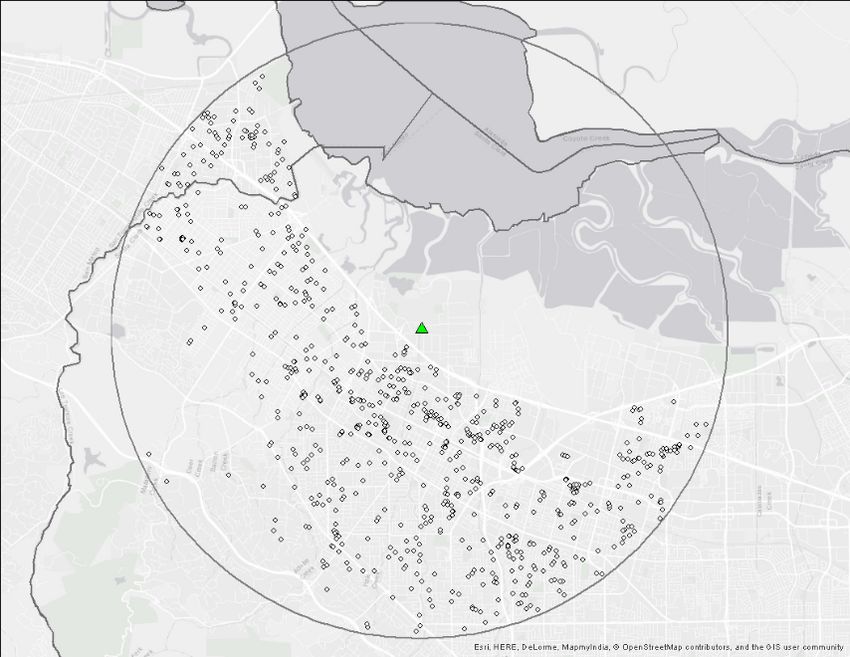
proximity to the firm, and the characteristics of firms and IPOs. The results for Silicon Valley are not

significantly different from those for California. Based on the baseline estimation using the county control

group, the effect is largest for share issuing events: 3.3%, 1.7%, and 1.3% for a 1-. 5-, and 10-mile radius,

respectively, based on the 90-day pre- and post-event windows. This result is consistent when zip code areas

are alternatively used as the control group. The monotonic decay by distance is consistent with original

shareholders’ preferences for proximity although the standard errors are large for a 1-mile radius.7 The

effect is also large for IPO filing events: 2.2%, 1.3%, and 1.6% for a 1-. 5-, and 10-mile radius, respectively.

However, the effect of lock-up expiration events is smaller: 0.1%, 1.4%, and 0.8%. These effects based on

HPIs are estimated for the houses with the same observed characteristics, but we also confirm that the

average characteristics of transacted properties do not significantly change after IPO events.

    However, there is a concern that the location near IPO firms’ headquarters may have a higher baseline

growth rate of house prices regardless of IPOs due to some unobservable factors. For example, IPO firms

may have chosen the high-amenity locations that tend to exhibit large property price appreciation. Although

firm fixed effects capture unobserved locational heterogeneity in price levels, there may still be heterogeneity

in growth rates. When we estimate the HPI premium for the treatment area each month around an IPO

event, we observe both a discontinuity around an IPO event and a trend of widening gaps. Thus, we conduct

a placebo test by falsifying event dates while maintaining the correct locations.8 We find the baseline

premium in growth rate for the treatment area defined by a 1- to 2-mile radius. This baseline premium

is comparable in magnitude to the estimated treatment effect in our main result. However, the baseline

premium is significantly smaller (around 0.6%) for a 10-mile area. When we remove the baseline growth rate

premium from our main result for a 10-mile area, the average treatment effect is 1.0% for filing and 0.8%

for issuing, but approximately zero for lock-up expiration.

    This result suggests that original shareholders change their housing demand when their wealth changes

but not when liquidity constraint is relaxed. Because the original shareholders cannot cash out their wealth

at the time of share issuance or IPO filing, our result suggests that the original shareholders can finance

their home purchases based on their illiquid wealth. It is unlikely that arbitrageurs (flippers) with enough

liquidity buy houses to make short-term profits because of large housing brokerage fees. Banks in California

may not be very restrictive in originating mortgages to entrepreneurs and workers at start-up firms because

of their relatively rich experience with this type of consumers. Thus, the result of no liquidity constraint

may not extend to other states. For example, in a related study, Hartman-Glaser et al. (2017) use the
   7 FigureA2 depicts the geographical decay.
   8A related concern is that the price increase after IPO events may not be specific to the location of IPO firm headquarters.
We conduct a placebo test by falsifying the location of an IPO firm’s headquarters while maintaining the correct event date
but do not find a significant change in house prices for the falsified locations.

                                                              3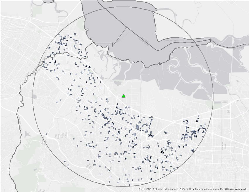
IPO and housing data for Denver, Colorado, and find a larger treatment effect for the lockup expiration

event than for the filing and issuing events. Although this difference between California and Colorado is not

conclusive because of differences in data sources and estimation methods, this contrast is very suggestive of

the uniqueness of mortgage origination markets in California.

   The effect of IPOs on house prices varies by firm and IPO characteristics. The effect is generally larger for

younger and smaller firms than for older and larger firms. For example, when firms are younger than the first

quartile, there is a 2.8% increase in house price levels around the issuing event, which is 3.8 times the increase

for the firms older than the third quartile. This result is consistent with the observation that managers and

workers at start-up firms prefer to live closer to the firms. The treatment effect is also positively related with

offer price, IPO proceeds, and the degree of underpricing at filing, all of which represent the size of wealth

increase by IPOs. The IPOs with secondary share offering and no lockup restriction suggest that original

shareholders can monetize their wealth immediately after share issuance. These characteristics are associated

with a unique pattern of house prices. Although they are not associated with the price change after IPO

events, they are associated with significantly lower house prices during the six-month period around filing

and significantly higher prices during the six-month period around issuing. These results are consistent with

a possibility that home purchases are delayed until debt financing is available just before share issuance, but

micro-level buyer data are needed for a conclusive analysis.

   We also examine the relation between the treatment effect and IPO performance as measured by the

stock price return over the offer price and its volatility. Based on a 5-mile radius within a 90-day event

window, a one-percentage point increase in returns is associated with a 1.4% larger treatment effect around

the IPO issuing event and a 0.7% larger effect around the lockup expiration event. This result supports

the wealth hypothesis. In contrast, the stock return volatility does not create a significant difference in the

treatment effect. However, greater volatility is associated with larger HPIs around headquarters both before

and after a lockup expiration date. This finding is consistent with the hypothesis that original shareholders

with volatile wealth diversify their portfolios into housing at either filing or issuing.

   In summary, the evidence supports an expectations hypothesis, in which the original shareholders without

liquidity constraints change their demand for housing consumption at the IPO filing event. The evidence

also supports a wealth hypothesis, in which the original shareholders change their housing demand when their

book value of wealth is determined in the stock exchange. However, the evidence does not support a liquidity

hypothesis, in which the original shareholders change their housing demand only when they can monetize

their book wealth. In general, IPOs partly explain the appreciation of local housing prices.

   This paper contributes to the literature in two ways. First, to our knowledge, this is the first study that

identifies a causal effect of IPOs on local house prices. We demonstrate that positive correlations between

                                                        4
IPOs and home price appreciation cannot be entirely attributed to the causal effect of IPOs. On average,

we find a 1% effect of a filing event and a 0.8% effect of a share issuing event; i.e., a 1.8% increase in local

house price around IPO firms’ headquarters for each IPO. Second, different IPO events provide a unique

setting for comparing the impact of wealth and liquidity constraints. Our findings indicate that original

shareholders in California shift their housing demand when a future wealth increase is anticipated and when

a wealth increase is confirmed regardless of weather wealth is immediately available. This result suggests

that personal financing function well for high-wealth individuals in California, allowing them to smooth

consumption.

     The paper is structured as follows. Section 2 provides institutional background and sets up the hypothe-

ses. There is a discussion about the data and methods in section 3, which includes summary statistics. The

main results are presented in section 4. In section 5 the treatment is decomposed at the property transaction

level by market segment and composition. Finally, there is a concluding section.

2      Background and Hypothesis Development

     Underwriting standards in mortgage lending and credit constraints in home purchasing are explicit and

uniformly applied. For example, the down payment constraint also known as loan-to-value (LTV) thresholds

limit the amount of a property’s sales price that a borrower can finance and impose additional costs for

higher LTV loans.9 Also, the debt-to-income (DTI) restriction limits the amount of outstanding debt that

a borrower can have in proportion to their income.

     The LTV and DTI constraints are most likely to affect original shareholders. First, original shareholders

are unable to use pre-IPO shares and firm equity for a down payment. Second, stock options that compensate

original shareholders with equity substitutes for cash compensation. In the case of cash constrained start-

ups, they are more likely to compensate employees with stock options where the larger the proportion of

compensation to original shareholders is in the form of stock options increases the likelihood of a binding

DTI constraint because it lowers the amount of housing services that original shareholders can purchase as

a function of their income. As a result, original shareholders are disproportionately likely to be bound by

credit constraints that lead them to forego housing consumption today. In addition, to smooth consumption

original shareholders are more likely to use their stock options and equity stake as a mechanism to save for

a down payment. Therefore, by saving less of their income original shareholders are able to smooth their

consumption.

     Under the null hypothesis, there is no association between property values and IPOs.
    9 For
       example, loans with an LTV in excess of 80% are charged private mortgage insurance (PMI) that is added to the
monthly mortgage payment as a percentage of the loan amount.

                                                         5
H0 : (Null Hypothesis) There is no change in property values associated with IPO events.

    In this case, the credit constraints are not binding and there is no unexpected changes to the personal

wealth of original shareholders that would lead them to change their demand for housing services. If there is

evidence of a post-treatment effect then we reject the null hypothesis in favor of the alternative that either

there are binding credit constraints or there is an unexpected wealth shock.

    In rejecting the null hypothesis in favor of the alternative that IPOs influence local housing markets,

there are three mechanisms that may be driving the treatment effect that are not mutually exclusive. These

are the expectations, wealth, and liquidity hypotheses, which closely follow from the sequential events of a

completed IPO.

    First, a firm declares their intent to go public. The firm is signaling that their IPO is imminent and

removing uncertainty about the timing and exit strategy for original shareholders.10 Using the date when

Form S-1 is submitted as the IPO filing event, we define the expectations hypothesis as a change in the

demand for housing from this updated expectation.

H1 : (Expectations Hypothesis) There is a change in local property values following the submission of Form

      S-1.

A change in expectation increases the demand for housing if credit constraints to acquire financing are not

binding. In this case, original shareholders can adjust their consumption of housing services even if wealth

cannot be immediately monetized.

    Second, at the IPO event the firm issues equity and they are listed on an exchange. At this point, any

uncertainty around the firm’s market value is removed as well as the uncertainty about whether the firm

would successfully IPO.

H2 : (Wealth Hypothesis) There is a change in local property values after the firm’s shares are listed on a

      public exchange when an unexpected change to original shareholders’ book value of wealth leads to a

      change in their demand for housing.

    There are two possible reasons for a change in house prices around the issuing event. First, original

shareholders changer their housing demand in response to the realization of a wealth shock from the IPO

when their book value of wealth is determined in the stock exchange. An unexpected change impacts the

consumption and tenure choice of original shareholders in the post-IPO period (Friedman, 1957). Second,

if there were binding constraints in the pre-IPO period that no longer bind. For example, if the firm’s
  10 If original shareholders consider the present value of the payoff from the IPO as the discounted sum of the probability

that the firm IPOs in each period then filing increases the present value of the payoff by significantly reducing the number of
discounted periods.

                                                              6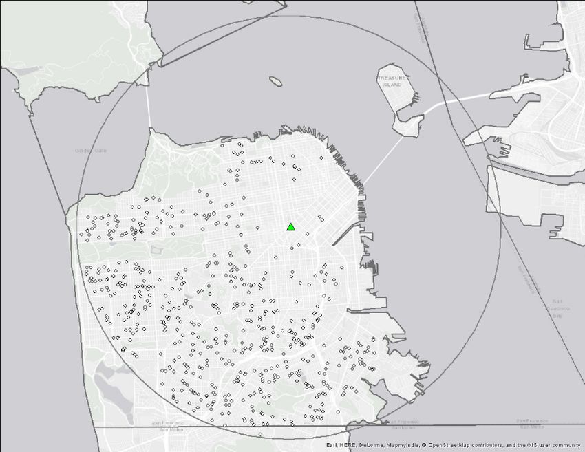
listing occurs at the same time that they make significant changes to the compensation structure for original

shareholders. However, original shareholders’ wages are unlikely to change around the IPO event and in the

presence of a lockup restriction their pre-IPO shares cannot be liquidated to go towards a down payment.

Under the wealth hypothesis changes in property values around the IPO event are due to unexpected changes

in the book value of wealth for unconstrained original shareholders that lead to changes in the demand for

housing.

   At this point, wealth-constrained original shareholders respond to changes in their illiquid assets whereas

liquidity-constrained original shareholders will not (Tobin, 1972). The presence of a lockup restriction may

lead original shareholders to be liquidity constrained because they are unable to liquidate their equity position

in the firm until the lockup period expires. During this period, which is usually 180 days between the IPO

and the expiration of the lockup, original shareholders are restricted from selling and cashing-out their

shares. In some cases, there are IPOs that do not have a lockup period but that is not the norm. The

lockup period benefits original shareholders by signaling the firm’s quality to investors, aligns incentives,

and protects underwriters.

   However, firms can offer existing “secondary shares” at the IPO from original shareholders to the public

in addition to new “primary shares” that allows original shareholders to liquidate their pre-IPO shares at

the issuance when a lockup restriction is present. In this case, the lockup restriction does not apply to

this subset of original shareholders. In Chua and Nasser (2016) does find that original shareholders are

motivated to offer secondary shares by apparent liquidity needs. For example, smaller cash-pay is associated

with larger secondary offerings. However, secondary shares are viewed negatively by investors and Aggarwal

et al. (2002) demonstrate that it is optimal for managers to wait for the end of the lockup. Therefore, the

majority of firms do not offer secondary shares and when they do it tends to be only a small proportion of

original shareholders that have this opportunity (Field and Hanka, 2001).

   Third, the lockup event occurs when the limits on original shareholders’ trading restricted shares ex-

pires.11 To restricted shareholders, the only difference between immediately before and immediately after

the lockup expiration is their ability to liquidate their restricted shares. Under the liquidity hypothesis there

is a change in the demand for owner-occupied housing following the expiration of the lockup restriction when

liquidity constrained original shareholders are no longer subjected to binding credit constraints.

H3 : (Liquidity Hypothesis) Higher property values follow the expiration of the lockup period.

   We assume that the wealth associated with the restricted shares is either not fungible or is costly to access.

However, there is a concern that the lockup event is associated with additional potentially confounding
 11 When  more than one lockup expiration date appears in the IPO data from SDC the first incidence is considered as the
lockup expiration date for that IPO.

                                                           7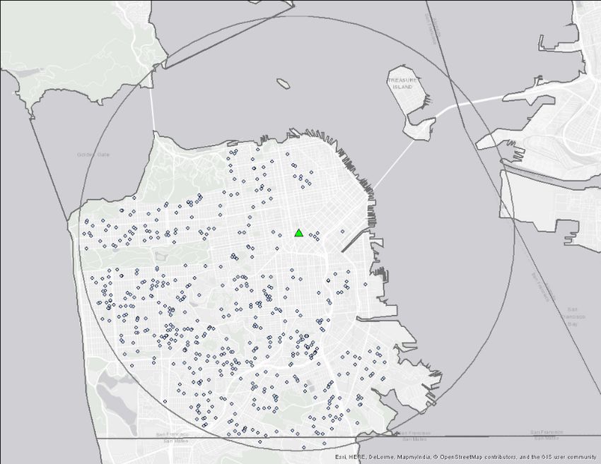
treatment effects. For example, Field and Hanka (2001) find an abnormal three-day return of -1.5% from

looking at the returns around lockup expiration events. Therefore, changes to original shareholders’ wealth

consistent with an abnormal negative return around the lockup expiration only biases against finding evidence

supporting the liquidity hypothesis.

    The lockup period acts as a triggering event similarly to the down payment requirement. Artle and

Varaiya (1978) show how down payments deter home ownership when the benefits from ownership do not

exceed the loss in utility from having to save. Therefore, individuals make tenure choices as soon as they

reach the down payment threshold associated with their demand for housing consumption where the down

payment acts as a triggering event. Similarly, when original shareholders are liquidity constrained such that

credit constraints are binding then they are unable to fulfill their demand for housing services until the

lockup expires, which then acts as a trigger event. The question about the magnitude and significance of

the impact on local housing markets is an empirical one.

3     Methodology and Data

    We follow a hedonic approach for modeling house prices to test for an association between IPOs and

local house price changes. Rosen (1974) is credited with developing the hedonic price method that assumes

property values can be regarded as the sum of implicit prices of a bundle of attributes in equilibrium. It is

a common method applied in housing related research.

    However, there is an omitted variable concern when prices and implicit goods are determined in a spatial

equilibrium. In this case, if the choice of the firm’s location correlates with the timing of the IPO; if the

timing of the IPO correlates with local housing market cycles; or they both correlate with an unobserved

omitted variable then the estimates for treatment will be biased.

    Our main concern is that the timing of an IPO and the location of the firm are choice variables that are

endogenous. In Brau and Fawcett (2006) they survey chief financial officers (CFOs) and find that creating

shares for acquisitions is the most important motivating factor for going public where the overall stock

market and industry performance are the largest determinants of IPO timing. Therefore, IPOs are not

timed in coordination with house prices directly but the determinants of IPO timing may still correlate with

an omitted variable that correlates with local property values.

    To deal with this problem, we exploit spatial-temporal variation of IPOs. The approach is similar to Pope

and Pope (2015) that looks at Walmart openings and compares transactions that are closer to a Walmart to

those slightly farther away before and after it opens. Other studies with similar designs have looked at the

impacts of sex offenders (Pope, 2008), the spillover effects associated with foreclosures (Gerardi et al., 2015;

                                                       8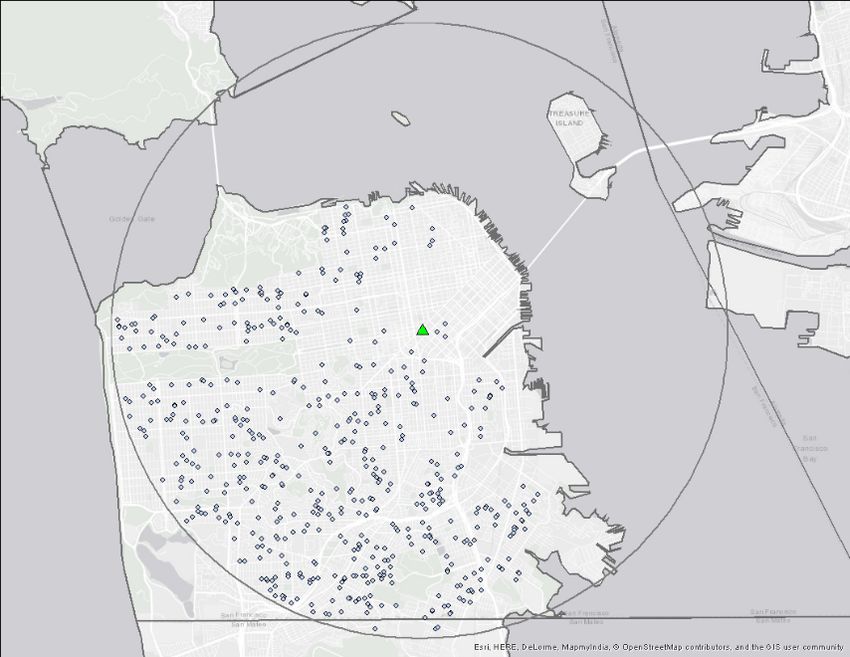
Lin et al., 2009; Schuetz et al., 2008), and forced sales (Campbell et al., 2011). In our case, we construct

IPO specific house price indexes that capture the trend of house prices on the treated population around

the firm’s headquarters and then control for general house price trends with the complementing county level

HPI.

   This difference-in-differences approach requires two assumptions for a causal interpretation of the results.

First, original shareholders are assumed to value proximity to the firm’s headquarters, ceteris paribus. As

long as they place some cost on the time they spend commuting and there is an association between distance

and commuting time this assumption holds. Second, we attribute changes in house prices levels right before

and right after an IPO event to the IPO event itself. By only including transactions that occur around

the IPO event date being considered and within 5 miles of the firm’s headquarters limits the possibility of

confounding events. This approach controls for the trend in house prices and time invariant omitted variables

related to the firm’s location.

   Also, we consider each IPO as three separate event studies corresponding to the sequential events of a

completed IPO. In this way, the IPO events being considered do not occur simultaneously with the decision

to go public. Instead the time between the decision to go public and the each IPO event varies by event and

by firm. For example, the length of time between the filing event and issuance depends on the length of time

that managers spend with underwriters on the road show gauging investor interest. Then after the firm is

listed, the time between IPO issuance and the expiration of the lockup period is generally 180 days, which

is defined by institutional convention and not from any consideration of local house prices. As a result, the

length of time between IPO filing and the expiration of the lockup period can span years and there is no

indication that IPOs are timed with the local housing cycle over the course of the IPO events. Therefore, it

is assumed that IPO events are exogenous shocks to the local housing market.

3.1    Data and Summary Statistics

Transaction Level Data

   We use Zillow residential property level data for California. It is the product of merging their transaction

and property assessment files. In the raw file there are 12.8 million transactions with 99% falling between 1993

and 2017. The observations are cleaned on missing and unwanted or unreasonable property characteristics.

For example, intra-family transactions are excluded. Also, properties are filtered by property type, the

number of parcels, and the number of buildings. We restrict the sample to single parcels where there is

only one building and include property types: residential general, single family or inferred single family,

rural residence, townhouse, row house, planned unit development, and bungalow. The final sample consists

                                                       9
of properties that: have at least one full bathroom and at least one bedroom, non-negative property age
and less than or equal to 150 years old, non-missing sales price greater than or equal to $1,000, not more
than four units, non-missing latitude and longitude, non-missing land size strictly greater than 500 square
feet, and non-missing number of stories less than or equal to three. The final sample has around 6.5 million
unique property transactions from 1993 to 2017.
Initial Public Offering (IPO) Data
From SDC, we obtain 1,987 unique IPOs for California from 1970 through 2017.12 This list of IPOs is
filtered for missing address information, when a P.O. Box is listed as the firm’s address, and when geocoding
returns a less than to the street address level accurate longitude and latitude.13 Ultimately, the final sample
includes 725 IPOs from California with an IPO event between 1993 and 2017.
We summplement the IPO data from SDC with data from CRSP and from data available from Ritter.14
From CRSP, we obtain the daily open and closing stock prices, returns with and without dividends, the
number of shares outstanding, and the volume of shares traded. From Ritter, we obtain the firm’s founding
year and rollup status.15 From the 725 unique IPOs: there are 224 firms that offer secondary shares at the
IPO; 447 that are identified as being backed by venture capital; 71 where the IPO issue is backed by private
equity; and 16 identified as being rollup firms.
Summary Statistics
Table 1 summarizes the distribution of transactions and IPOs by year and by IPO event. It does appear
that the IPOs come in waves with the most filings in 1999 at the peak of the dot-com bubble and smaller
waves around 2004 and then again around 2014. Therefore, our period of analysis covers multiple cycles and
market environments including the financial crisis period.
Descriptive statistics are provided in Table 2 at the property and firm level. Panel A summarizes the
transacted properties where the average sales price over this period is $335,145. After adjusting for inflation
the average adjusted sales price over this period is $415,363.16 For the analyses, the adjusted sales prices
are used to generate the results althought they are robust to using the raw sales price. In terms of property
characteristics, there are large standard deviations but they are inline with similar studies.
Panel B summarizes the sample of IPOs where the average target price is $12.99 per share with a max
12 See figure A1 of the appendix for a comprehensive summary of the SDC IPO search criteria.
13 The Google maps geocoding API was used to return longitude and latitude of the firm’s listed address.
14 The Field-Ritter data on IPOs was downloaded (10/21/2017) from: https://site.warrington.ufl.edu/ritter/ipo-data/
15 A rollup is a firm that grows by acquiring other firms.
16 Sales prices are adjusted by finding the 05/2017 dollar equivalent according to the monthly Consumer Price Index (CPI)
for All Urban Consumers: All Items from https://fred.stlouisfed.org/series/CPIAUCSL (downloaded 7/19/2017).
10of $97.00 and average proceeds from the IPOs of roughly $131 million. There is a lot of variation within
IPO and firm level characteristics exhibited by the large ranges and standard deviations. For example, the
average for total assets is $224.24 million where the minimum is $0.10 million and the maximum is $7,190
million for the largest firm by total assets. We will exploit the variation in firm and IPO characteristics in
robustness tests to further examine the relationship between IPOs and local house prices. Specifically, we
focus on the variation in firm age, total assets, offer type, offer price, IPO proceeds, IPO underpricing, and
the firm’s stock performance post-IPO.
Panels C and D provide additional summary information about the performance of the IPO. The average
return at 1 year from the IPO is 25.47% with a minimum return of -227.78% and a maximum of 740.83%.
Here the firm’s return is calculated as the percentage change from the offer price to the closing price on the
date considered (i.e. 1 year following IPO) and the displayed average return is the simple average across the
firm’s. To quantify the risk associated with the IPO, we calculate the relative volatility for each firm’s stock
post-IPO as the standard deviation of daily closing prices divided by the average of closing prices for the
period.
Event Level Statistics
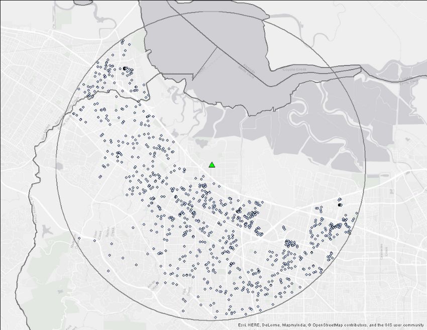
Table 3 shows mean differences in adjusted sales prices of transactions in a pre or a post-period by event
type and across distances of 1, 5, and 10 miles from the IPO firm’s headquarters. Specifically, transactions
are identified as occurring in a pre or post event window if they are within a specified radius of a firm’s
headquarters (1, 5, or 10 miles) and the sales date for the property is within 90 days of that firm’s IPO event.
For example, for Facebook’s IPO case, we define a 5-mile radius from Facebook’s headquarters and identify
property transactions that occurred within 90 days before and after Facebook’s IPO filing event (Figure 3).
We repeat this procedure for each IPO firm (e.g., Figures 4 and 5). It is possible that a transaction will be
included in the pre-period for one IPO and the post or treatment period for another. For this table, we only
include those observations that are in one pre-period or one post-period window by event type for a clean
interpretation of treatment. For example, a transaction that appears in the pre-lockup expiration period
for XYZ and the post-lockup expiration period for another IPO is excluded from this table summary of the
lockup event. Instead the main results are based on house price indexes that are generated at the firm event
level where overlapping observations are not excluded.
In Table 3 the post-filing prices are consistently higher than the corresponding pre-filing prices or roughly
a 3.7% increase in unconditional mean at 1 mile, which falls to 2.8% and 1.3% at 5 miles and 10 miles
respectively. The lockup expiration event shows a consistent negative price change in local house prices
across the distances with the largest decrease or -6.5% at 1 mile around the firm. The change around the
11issue date varies from negative at 1 mile and 10 miles but is positive at 5 miles. The largest magnitude of
price change around the issue date is -2.4% within a 1 mile distance boundary from the firm. To control
for differences in the composition of properties transacted and trends in house prices in the pre versus
post-period by IPO event additional analysis is necessary.
4 Constructing the IPO Event HPIs
We construct by firm (f ) by event (e) level house price indexes (HP If etd ). These house price indexes
by firm and by IPO event are generated following the time dummy approach and only those observations
identified in the firm’s pre or post-period by IPO event are included. It is a log-linear specification that
includes controls for property characteristics (Xi ) and time dummies that are defined in event time:
5
X
ln(Pit ) = β0 + uXi + δt Tit + εit . (1)
t=1
The dependent variable is the natural log of the adjusted sales price (Pi ) for property i and the time
dummies (Tit ) specify 30 day buckets from the IPO event. The property level controls (Xi ) capture observable
differences due to: land sf, total number of rooms, number of bedrooms, number of full bathrooms, number
of half bathrooms, age, the number of stories, property type, and county fixed effects. Because IPO events
do not coincide with calender dates, we impose an event time and bucket transactions into 30 day intervals
from the IPO event date. Therefore, the coefficient estimates over time (δ̂t ) give the variation in house
price levels over time relative to the base period, which is -90 to -60 days from the IPO event. This base
model is estimated for each firm (f ) and IPO event (e) to construct firm event level house price indexes
(HP If etd = 100 · exp(δ̂t )) by distance (d) from the firm.
In addition, we generate the complementing HPI or comparable county level house price indexes by firm
by event (HP Ifc etd ). The county level HPIs are unique to each firm (f ), event (e), and boundary specification
(d) so as to be consistent with the firm event level house price indexes (HP If etd ). The county level HPI
is defined as the complement of the transactions that are used in the construction of the firm event level
HPI (HP If etd ). For example, the county level HPI for IPO XYZ’s filing event includes the transactions not
included in the sample used to generate XYZ’s filing event HPI but that are in the same counties and over
the same pre and post-period.
We first present the main result for the average treatment effect on the treated followed by several
robustness checks. We then expand on the base model and test for an association between treatment and
firm characteristics, IPO characteristics, and IPO performance.
124.1 Main Result
To identify the conditional average treatment effect on the treated, we estimate the following base model
by IPO event:
HP If etd = β0 + β1 P ostf e + β2 HP Ifc etd + ηf + εf et (2)
The left-hand variable (HP If etd ) gives the time series of house price levels over the performance window.
When the performance window is defined at ±90 days and the HPI is defined at 30 day intervals then there
are 6 observations or house price levels per firm event. The dummy variable P ostf e identifies the post-period
by firm (f ) and event (e). Including the county level HPI complement (HP Ifc etd ) controls for house price
trends and the fact that the IPO events across firms do not occur simultaneously reduces the concerns of
confounding events. Also, firm fixed effects (ηf ) are included to control for firm level variation.
Table 4 displays the base model results by IPO events at 1, 5, and 10 mile boundary specifications.
According to the adjusted R-squared, the base model explains a significant amount of the variation in house
price levels around a firm’s headquarters around IPO events. The variable of interest, in this case, is the
post-period indicator that identifies the treated population of transactions occurring in the post-period.
Across the IPO events the coefficient estimate for the post-indicator for treatment is positive and tends to
be statistically significant at the 1% level. There is a 1.3% increase at 5 miles associated with the post-period
compared to the pre-period following the filing event that is statistically significant at the 1% level. The
strongest magnitude appears after the issue date within 1 mile where there is a roughly 3.3% increase in the
3 months following the issuing date. Also, the treatment effect is monotonically decreasing with increasing
distance or 1.7 and 1.3 at 5 and 10 miles respectively. Around the lockup expiration event, the treatment
effect of post-lockup restrictions is 1.4% at 5 miles and 0.8% at 10 miles with the 1% significance level.
Thus, we fail to reject the null hypothesis as the results from the base model specification are consistent
with the alternative hypotheses of changing expectations following the filing event, a wealth shock present
around the issuing event, and the removal of a liquidity constraint around the expiration of the lockup
restriction.
4.1.1 Tests for Changes in Transaction Characteristics
Since our main result is based on quality-controlled house price index, our estimates are not influenced
by potential changes in the average transaction characteristics before and after an IPO event. However,
potential changes in the average characteristics of house transactions are important when we are concerned
about the aggregate impact of IPOs. For example, if the average size of traded properties is larger in the
13post-period, there is an additional composition effect of IPOs on housing markets.
Following Pope and Pope (2015), we estimate the following model to test for changes in the composition
of transacted properties in the housing market from the pre to the post-period.
P ropCharif = β0 + β1 Postif + cntyi + ηf + εif (3)
We examine the treatment effect on the property characteristics (P ropCharif ) including ln(finished sf),
stories, total rooms, number of bedrooms, number of full and half bathrooms, and age. Firm and county
fixed effects control for the spatial and temporal variation by IPO event and the errors are clustered at the
firm level. Table 5 shows the result. We conclude that there is not a significant change in the composition of
properties being transacted after an IPO event for all event types. Only age is significant but we do expect
the population of post-period properties to be older from the event study design being in time.
4.1.2 Robustness Check by Zip-Code Control Area
As a robustness check, we estimate Equation (2) by defining the control area by zip code. Table 6 displays
the result. The result is qualitatively consistent with the main result. The estimated coefficients on Post
Event Date are statistically significant for all IPO events and the treatment area size. For example, the HPI
for the treatment area defined by 10 mile boundary is 1.7% higher after IPO filing, 1.9% higher after issuing,
and 1.3% higher after lockup expiration than the HPI for the control area in the same county.
4.1.3 Robustness Check by Transaction-Level Data
As a robustness check, we estimate the base model at the property transaction level. We use the obser-
vations that appear only in a single pre- or post-period window to remove the effect of overlapping multiple
events.
ln(Pif ) = β0 + β1 Postif + β2 HP Ifc etd + uXi + ηf + εif (4)
The dependent variable is the natural log of the adjusted sales price (Pif ) for property i that falls in the
IPO event window for firm f . Equation (4) includes covariates for property characteristics (Xi ), firm fixed
effects (ηf ), and the firm event HPI county complement (HP Ifc etd ).17 The transaction-level result shown in
Table A1 is consistent with the main result.
17 The controls for property characteristics (X ) include: land sf, total number of rooms, number of bedrooms, number of full
i
bathrooms, number of half bathrooms, age, the number of stories, property types, and county.
144.1.4 Robustness Check by Monthly Estimates
The main result is based on the average HPI during the 90-day post event period compared with the base
HPI measured at 90 days before the event. However, there may be gradual or non-monotonic price changes
around an event date because of information spillover or other factors affecting the market microstructure.
Thus, we estimate the monthly difference in HPIs between the treatment and control areas. Figure 6 depicts
the estimation result.
We confirm that the house price premium for the treatment area significant increases at the event date.
For filing events, the house price premium is not significantly different from zero before the event date based
on two standard deviations. However, the premium becomes statistically significant after the event date.
We also find the same result for issuing events and lockup expiration events.
At the same time, we also observe gradual increase in home price premia before and after the event
date. Unlike in a liquid and informationally efficient financial market, a gradual drift after an event is not
inconsistent with the treatment effect of an event in a housing market. For example, the original shareholders
may not be able to purchase a house at an event because it may take several months to find the best suited
house in housing markets. Furthermore, arranging a mortgage and making a purchase agreement usually
takes additional time. The price may also drift up before an event if the IPO event is highly anticipated. As
an anticipated IPO event approach, banks may become more willing to originate mortgages to the original
shareholders. Alternatively, there may be housing speculators who purchase houses in anticipation of a
future IPO event.
However, it is also possible that there is an unobserved difference in the growth condition of housing
markets between the treatment and control areas. For example, headquarters locations may have high urban
amenities and attract more wealthy residents regardless of IPO events. Alternatively, an IPO firm is located
in the area where housing demand is rapidly growing because of high amenities. To address this possibility,
we conduct several placebo tests. We report the result in the next section.
4.1.5 Robustness Check by Placebo Tests
We conduct placebo (falsification) tests to address the following concerns. First, unobserved housing
market conditions may generate different baseline growth in house prices around headquarters locations.
Second, the management choice may be endogenous as to when they pursue an IPO and where they locate
the firm’s headquarters.
We run two types of placebo tests. First, we estimate equation (2) for the firm’s true headquarters
location but at incorrect event dates through time or by pseudo-random date assignment. Then, we compare
15the falsified estimation results with our primary results based on the true IPO event dates. Second, we
randomly assign the latitude and longitude of the firm’s headquarters and estimate equation (2). Then, we
similarly compare the falsified estimation results with our primary results based on the true headquarters
locations. The detail of the falsification procedure is described in Appendix B.
Figure 7 depicts the result of the first type of placebo tests based on 90-day windows around falsified
event dates. Each panel shows the treatment effect with two-standard-error bands for the true event date
(at the value of 0 on the horizontal axis) and for falsified event dates (from −730 days before the true event
date to 730 days after the date).
For filing, the true treatment effect for a 10 mile boundary is clearly larger than the effects around falsified
dates. The average treatment effect for falsified event dates is 0.59% whereas the true effect is 1.59%. The
1.00% difference is sufficiently large relative to the average of standard errors (0.18). Thus, although there
seem to be a baseline difference in home price growth rates between the headquarters location and other
ares, a large deviation in home price growth occurs only around the true IPO filing date.
Similarly, for share issuing, the treatment effect at the true event date is 0.76 points larger than the
baseline premium in home price growth rates. However, the difference is not large for lockup expiration.
Table 7 shows the result for other sizes of the treatment area. The true treatment effect is significantly
larger than the baseline premium only for 3 miles or more around issue dates and for 10 miles around filed
dates. The effect of lockup expiration is also generally larger than the baseline premium, but the additional
increase in house price is not large. Thus, we can conclude that IPO filing and issuance affect the surrounding
housing market of a 10-mile radius by 1% and 0.8%, respectively. However, IPO lockup expiration does not
significantly impact the housing market in California.
Table 8 shows the result of the placebo test by 20 falsified headquarters locations. The average treatment
effect for falsified locations is not statistically significant relative to the standard deviation for any IPO event
and any boundary distance. For example, based on a 10-mile boundary, the average estimate for 20 locations
is 1.43% for filing whereas the standard deviation of estimates is 1.65%.
4.2 Variation By Firm Characteristics
In terms of firm characteristics, firm age is a likely proxy for growth and time at the headquarters while
total assets is a proxy of firm size. For example, growth firms can be cash constrained and thus rely more
heavily on stock options to compensate original shareholders. Because firm level characteristics may not be
linearly related with the treatment effect, we sort the firms into buckets by quartiles of the characteristic
of interest and estimate the base model (2) for each bucket. We demonstrate the results for a boundary
16specification of 5 miles.18
(Firm Age) Table 9 shows the coefficient estimates of treatment by firm age quartile by event where
firm age is defined as the difference between the founding year and issue year.19 The coefficient estimate
for treatment is consistently positive across the events and tend to be statistically significant. The youngest
quartile of firms exhibits the largest magnitude coefficient estimates of treatment across the IPO events
or 1.8% increase following the filing date, 2.8 after issuance, and 2.1 after the lockup expires where these
estimates are significant at the 1% level. Therefore, firm age is correlated with the treatment effect and
explains additional variation in house price levels.
(Total Assets) Firms are sorted into quartiles by their total assets where the firm’s total assets is measured
prior to going public. Table 10 gives the estimates of treatment by total asset quartile where the association
between firm size and the treatment effect is mixed.20 Smaller firms appear to exhibit larger magnitude
treatment effects. Around the issuing date the lowest quartile exhibits the highest post-period level change
of 2.2%. One concern is that firm size is only loosely associated with the size of the firm’s headquarters. For
example, larger firm’s may be more likely to have offices spread across regions.
4.3 Variation By IPO Characteristics
The characteristics of the IPO are associated with the size of wealth shocks to original shareholders and
the extent to which original shareholders are liquidity constrained. First, we proxy the magnitude of wealth
shocks by using the amount of proceeds, offer price, and the degree of underpricing at issuance. Second, we
examine the degree of liquidity constraint by identifying whether an IPO involves secondary share offerings
and lockup restrictions. Our sample of 725 unique IPOs includes 152 IPOs without a lockup period and
224 IPOs with secondary shares offerings. Original shareholders are not subjected to liquidity constraint at
share issuance if no lockup restriction is imposed or their secondary shares are offered (Chua and Nasser,
2016).
(Proceeds) We predict that larger IPOs by total proceeds will be associated with larger treatment effects
similar to the expectation that larger firms by total assets would have a greater impact on the local housing
market. We construct subsamples by quartiles of IPO proceeds and estimate the base model (equation (2))
separately for each subsample. Table 11 displays coefficient estimates of the treatment effect when the IPOs
are sorted into quartiles by total IPO proceeds.21 A positive relation between proceeds and the treatment
effect is strongest for the filing event. The treatment effect is 1.8% and statistically significant at the 1%
18 Results at 1 and 10 miles are consistent with those at 5 miles and are available by request.
19 See Figure A3 in the appendix for a graphical representation.
20 See Figure A4 in the appendix for a graphical representation.
21 See Figure A5 in the appendix for a graphical representation.
17level for the largest quartile of IPOs by proceeds. However, the relation is not monotonic for the issuing and
lockup expiration events.
(Offer Price) Fernando et al. (2004) suggest that the offer price is informative and is associated with
institutional investment, underwriter reputation, and the mortality rates of firms. We construct subsamples
by quartiles of offer prices and estimate the base model for each subsample. Table 12 shows heterogeneous
results in the association between offer price, the treatment effect, and IPO events.22 For example, the offer
price and the treatment effect is positively related and increasing over the quartiles for the filing date. The
top quartile exhibits the largest magnitude of 1.8% and is significant at the 1% level. Similarly, for issuing
event, the treatment effect tends to be larger for larger offer prices. In contrast, the relation is opposite for
the lockup expiration; the treatment effect is larger for smaller offer prices.
(Underpricing) We define underpricing as the ex post percentage increase from the offer price to the
closing price on the issue date. Thus, the larger the underpricing, the larger the realized gain from the
IPO to original shareholders. Table 13 displays coefficient estimates of the treatment effect when firms are
bucketed into quartiles by IPO underpricing.23 For all three types of events, there is a U-shaped pattern in
the relation between the treatment effect and the degree of underpricing. For the filing and issuing events,
the treatment effect is largest for the IPOs with a largest degree of underpricing (1.9% and 2.5% for filing and
issuing, respectively). For the lockup event, there is insufficient evidence of the relation between underpricing
and the treatment effect.
To examine the variation by secondary share offerings and lockup restrictions, we estimate the following
variation of the base model that includes indicators for the presence of secondary shares and a lockup
restriction. In addition, these indicators are interacted with the indicator of treatment to give the differential
treatment effect.
HP If etd = β0 + β1 P ostf e
+β2 (P ostf e · SecShrsf ) + β3 SecShrsf
(5)
+β4 (P ostf e · N oLockupf ) + β5 N oLockupf
+β6 HP Ifc etd + ηf + εf et
The HPI complement (HP Ifc etd ) and firm fixed effects are included as controls with the displayed standard
errors are clustered at the firm level.24
(Secondary Shares) Table 14 shows the results from equation (5) where the main effect for secondary
shares is consistently significant at the 1% level. The coefficient estimate is negative around the filing date
and positive around the issuing and lockup events. This pattern is consistent with original shareholders
22 SeeFigure A6 in the appendix for a graphical representation.
23 SeeFigure A7 in the appendix for a graphical representation.
24 Results at 1 and 10 miles are consistent with those at 5 miles and are available by request.
18You can also read