PyFOOMB: Python framework for object oriented modeling of bioprocesses

Received: 20 November 2020 Revised: 9 December 2020 Accepted: 9 December 2020

DOI: 10.1002/elsc.202000088

RESEARCH ARTICLE

pyFOOMB: Python framework for object oriented modeling
of bioprocesses

Johannes Hemmerich1 Niklas Tenhaef1 Wolfgang Wiechert1,2,3
Stephan Noack1,3

1Institute of Bio- and Geosciences - IBG-1:
Biotechnology, Forschungszentrum Abstract
Jülich GmbH, Jülich, Germany Quantitative characterization of biotechnological production processes requires
2 Computational Systems Biotechnology
 the determination of different key performance indicators (KPIs) such as titer,
(AVT.CSB), RWTH Aachen University,
Aachen, Germany
 rate and yield. Classically, these KPIs can be derived by combining black-box
3Bioeconomy Science Center (BioSC), bioprocess modeling with non-linear regression for model parameter estimation.
Forschungszentrum Jülich, Jülich, The presented pyFOOMB package enables a guided and flexible implementa-
Germany
 tion of bioprocess models in the form of ordinary differential equation systems
Correspondence (ODEs). By building on Python as powerful and multi-purpose programing lan-
Stephan Noack, Institute of Bio– and guage, ODEs can be formulated in an object-oriented manner, which facilitates
Geosciences IBG-1: Biotechnology,
 their modular design, reusability, and extensibility. Once the model is imple-
Forschungszentrum Jülich GmbH, 52425,
Jülich, Germany. mented, seamless integration and analysis of the experimental data is supported
Email: s.noack@fz-juelich.de by various Python packages that are already available. In particular, for the iter-
Funding information
 ative workflow of experimental data generation and subsequent model param-
Bioeconomy Science Center, Grant/Award eter estimation we employed the concept of replicate model instances, which
Number: 313/323-400-00213; Bundesmin- are linked by common sets of parameters with global or local properties. For
isterium für Bildung und Forschung,
Grant/Award Numbers: 031B0463, the description of multi-stage processes, discontinuities in the right-hand sides
031B0918A of the differential equations are supported via event handling using the freely
 available assimulo package. Optimization problems can be solved by making
 use of a parallelized version of the generalized island approach provided by the
 pygmo package. Furthermore, pyFOOMB in combination with Jupyter note-
 books also supports education in bioprocess engineering and the applied learn-
 ing of Python as scientific programing language. Finally, the applicability and
 strengths of pyFOOMB will be demonstrated by a comprehensive collection of
 notebook examples.

 KEYWORDS
 bioprocess modeling, object oriented modeling, ODEs, Python

Abbreviations: ALE, adaptive laboratory evolution; CI, confidence
interval; IC, initial condition; KPI, key performance indicator; NLL, © 2021 The Authors. Engineering in Life Sciences published by Wiley-VCH GmbH
negative log-likelihood; ODE, ordinary differential equation

This is an open access article under the terms of the Creative Commons Attribution License, which permits use, distribution and reproduction in any medium, provided the
original work is properly cited.

Eng Life Sci. 2021;1–16. www.els-journal.com 1

2 HEMMERICH et al.

1 INTRODUCTION
 PRACTICAL APPLICATION
Biotechnological production processes leverage the
microorganisms’ synthesis capacity to produce com- Based on the powerful, yet beginner-friendly
plex molecules that are hardly accessible by traditional Python programing language, the pyFOOMB
chemical synthesis. Importantly, modern genetic engi- package addresses a wide range of users to imple-
neering methods allow for targeted modification of single ment bioprocess models with growing complexity.
enzymes and whole metabolic pathways for biochemically ODE models can be formulated in an object-
accessing value-added compounds beyond those naturally oriented manner, which facilitates their modular
available. However, to render the production of a target design, reusability and extensibility. pyFOOMB
compound economically feasible, a suitable biopro- supports the modeling of discrete behaviors in
cess needs to be developed which fits to an engineered process quantities, which is an important feature
microbial producer strain. In this context, computa- for the simulation and optimization of fed-batch
tional modeling approaches utilize existing knowledge processes. The concept of model replicates and
on strain and process dynamics, giving rise to modern definition of local and global parameters mirrors
systems biotechnology. Once a digital representation of a the iterative nature of data generation from cycles
biotechnological system has been implemented, in silico of experiment design, execution, and evaluation.
optimizations can be performed to design an improved Moreover, seamless integration with existing
bioprocess, effectively reducing the number of wet-lab and future Python packages for scientific com-
experiments. With the availability of new experimental puting is greatly facilitated. Most importantly,
data the computational model can be refined to increase the applicability and strengths of pyFOOMB is
its predictive power towards an optimal bioprocess. demonstrated by a comprehensive collection of
 Considering the highly interdisciplinary nature of sys- notebook examples.
tems biotechnology requiring expertise in (micro-)biology,
process engineering, computer science, and mathematics,
it becomes obvious that rarely a single person can have
a deep knowledge in all these fields. The more special-
 tion of ready-to-use working examples which come along
ized and performant a bioprocess model is intended to
 with pyFOOMB.
be, the higher the knowledge level needed by the user.
 Due to the full programatic access to Python, com-
This may prevent non-experts in modeling and programing
 plex models can also be implemented. Furthermore, great
from dealing with these highly rewarding topics. Conse-
 importance was given to convenient visualization methods
quently, there is a need for tools that can be quickly learned
 that facilitate the understanding of qualitative and quan-
and applied by non-experts, with the development of addi-
 titative model behavior. Finally, the enormous popular-
tional skills determined by demand.
 ity of Python as the de facto standard language for data
 Here, we present the pyFOOMB package that enables
 science applications makes it easy to integrate pyFOOMB
the implementation of bioprocess models as systems of
 with other advanced tools for scientific computing.
ordinary differential equations (ODEs) via the multi-
purpose programing language Python. Based on the object-
oriented paradigm, pyFOOMB provides a variety of classes
for the rapid and flexible formulation, validation and appli-
 2 MAIN FUNCTIONALITIES OF
cation of ODE-based bioprocess models. Table 1 gives a
 pyFOOMB FOR BIOPROCESS MODELING
comparative, non-exhaustive overview of software pack-
 Bioprocess models are implemented as ODEs for the time-
ages that are suitable for bioprocess modeling. These tools
 dependent variables ( ):
were developed with partly other application areas in
mind, e.g., modeling and analysis of biochemical networks
 
or simulation of chemical engineering unit operations. = ( ( ), , ), ( 0 ) = 0 (1)
 
Consequently, these software packages require different
levels of programing skills and some domain-specific ( ) = ( ( ), , ) (2)
knowledge for accessibility. Therefore, a major driver to
establish pyFOOMB was to provide a flexible modeling which depend on model parameters and initial values
tool that requires only basic programing knowledge and 0 . In practice, some of the variables might not be directly
thus shows low hurdles for beginners in bioprocess mod- measurable. Therefore, observation (or calibration) func-
eling. The latter is supported by a comprehensive collec- tions ( ) can be defined that relate these variables to

HEMMERICH et al. 3

TA B L E 1 Non-exhaustive comparison of software packages suitable for bioprocess modeling
 Main user
 Tool Description Languages interface License
 AMIGO2 [1, 2] Provides relevant methods around ODE modeling MATLAB MATLAB editor Free for
 like model calibration, uncertainty analyses, academic
 (multi-objective) optimal experimental design. users
 Definition of global and local parameters among
 different experiments.
 AMICI [3, 4] Interface to SUNDIALS integrators for efficient C++, MATLAB, MATLAB editor, BSD3-Clause
 simulation and sensitivity analyses with analytical Python Jupyter
 gradients (forward, 1st and 2nd order adjoint notebook, Python
 sensitivities) for biological ODE models, support IDEs
 for SMBL models. Supports models with
 discontinuities and corresponding event handling
 for the MATLAB implementation.
 Berkely Standalone software with graphical interface for ODE Standalone, own GUI Commercial
 Madonna model development. Model construction via syntax for ODEs
 connection of library items, which auto-generates
 corresponding equations using a custom equation
 syntax. Comprehensive suite for different
 visualization tasks. Routines for curve fitting and
 parameter scanning. Automated model generation
 using conventional chemical notation.
 COPASI [5, 6] Developed for metabolic network analysis and Standalone, CLI, GUI Artistic License
 reaction compartment modeling in systems Python via 2.0
 biology, with provision of typical methods like PyCoTools
 EFM analysis and MCA. Definition of global and package
 local parameters among different experiments.
 Simulations of ODEs and stochastic kinetics.
 Support for SMBL models.
 DAE Tools [7, 8] Industry grade DAE modeling toolbox for chemical C++, Python Jupyter notebook, GNU GPL3
 engineering applications and beyond. Code Python IDEs,
 generation for export and co-simulation GUI
 capabilities via FMI. Python as modelling language
 and high-level access to performance modules
 developed in C++. Supports models with
 discontinuities and corresponding event handling.
 pyFOOMB Rapid prototyping of ODE bioprocess models and Python Jupyter notebook, MIT
 provision of typical methods (model calibration, Python IDEs
 sensitivity and uncertainty analyses). Supports
 ODE modelling with discontinuities and
 corresponding event handling. Definition of global
 and local parameters among different experiments.
 Low-barrier teaching into bioprocess modelling
 and programing. Modelling strictly follows the
 object-oriented approach. Depends on assimulo
 package interfacing SUNDIALS’ CVODE for ODE
 integration and pagmo2/pygmo package for
 parallelized optimization following the generalized
 island model.
The listed tools were developed for different application areas and address different primary needs. Therefore, domain-specific knowledge and programing skills
are required for the packages’ accessibility. All packages provide at least several functionalities required for bioprocess modeling.

4 HEMMERICH et al.

the observable measurements, thus introducing additional
parameters into the model.
 In order to make the user familiar with our pyFOOMB
tool, a continuously growing collection of Jupyter note-
book examples is provided. These demonstrate basic func-
tionalities and design principles of pyFOOMB and serve
as blueprint for the rapid set up of case-specific bioprocess
models (Table A1).

3 MODELING WORKFLOW WHEN
USING pyFOOMB

In the following we present a typical workflow for imple-
menting and applying bioprocess models with pyFOOMB
(Figure 1). Throughout this section the toy model of Fig-
ure 2A will be employed.

3.1 Model definition

In a first step, the targeted model and its parametrization
is implemented by creating a user-specific subclass of the
provided class BioprocessModel (Figure 2B). This basic
class provides all necessary methods and properties to run
simulations for the implemented model. Essentially, the
abstract method rhs() must be formulated by the user.
 Noteworthy, the pyFOOMB package does not allow for
consistency checking of units for the state variables or
model parameters. This responsibility is left to the user
while formulating a model, i.e., before coding the model
as BioprocessModel subclass.

3.1.1 Discrete behavior

To monitor and control the dynamics of specific model
variables so-called state_events() and change_
states() methods can be defined. This is for example
required for the modeling of multi-phased processes such
as fed-batch with event-based changes in feeding regimes.

3.1.2 Observation of model states

In order to connect the model variables to measurable
quantities, an ObservationFunction can be created, with
the mandatory implementation of the observe() method
for each relevant calibration function. Noteworthy, a vari- F I G U R E 1 High-level description of a typical bioprocess mod-
able’s state can be linked to different observation func- eling workflow with pyFOOMB. For a full description of all classes
tions, reflecting the fact that there are typically several and methods including a complete list of all arguments and default
analytical methods available for one specific bioprocess values, please see the provided Jupyter notebook examples and
quantity. This approach allows to separate the bioprocess source code documentation

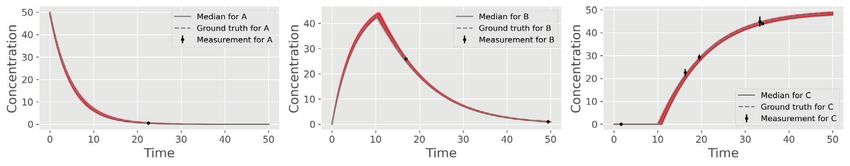
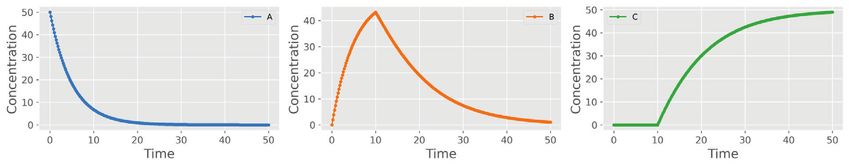
HEMMERICH et al. 5

F I G U R E 2 Toy example of a sequential reaction cascade. (A) Mathematical representation of the ODE system with initial conditions
(IC). (B) Object-oriented implementation in pyFOOMB. The ODE is defined within the rhs() method. Initial values and model parameters are
defined as dictionaries. (C) Results of a simulation. At = 10 an event occurs, where the conversion from B to C is switched on, i.e., 2 > 0

6 HEMMERICH et al.

model from corresponding observations functions and detection [9]. Its Python interface is provided by the
thus, increases re-usability of the different parts. By deriv- assimulo package [10], which implements seamless event
ing initial guesses for the parameters, a simulation from handling hidden from the user. Running some simulations
the model is typically used to verify the intended qualita- with subsequent visualization is a convenient approach
tive behavior in comparison to the experimental data. to verify the qualitative and quantitative behavior of the
 implemented model (Figure 2C).
 pyFOOMB provides a class with convenient methods
3.1.3 Global and local parameters for that purpose, e.g., plotting of time series data cover-
 ing model simulations and measurement data, corner
A key feature of pyFOOMB is the possibility to inte- plots for one-by-one comparison of (non-linear) corre-
grate measurement data from independent experimental lations between parameters from Monte-Carlo sampling
runs (replicates) by creating a corresponding number of as well as visualization of the results from sensitivity
new instances of the same model. These can still share analysis.
a common set of model parameters that are defined as
“global”, but at the same time differ in some other “locally”
defined parameters. 3.3 Sensitivity analysis
 Typical global parameters of an ODE-based bioprocess
model are the maximum specific growth rate max or Local sensitivities ( )∕ are available for any model
the substrate specific biomass yield X/S , while all initial response (model state or observation) with respect to
values are reasonable defined as local parameters (see any model parameter (including ICs and observation
Application example II). Different values for the local functions). The sensitivities are approximated by the cen-
parameters reflect biological or experimental variability tral difference quotient using a perturbation value of ℎ ⋅
that may arise from slight deviations in preparing, run- (1, | |). Sensitivities can also be calculated for an
ning or analyzing each replicate experiment. Alternatively, event parameter that defines implicitly or explicitly a point
such variability might be introduced by purpose when in time where the behavior of the equation system is
conducting replicate experiments with intentionally very changed (cf. Figure 3A). This is useful for, e.g., analyzing
different starting conditions. The latter refers to a classical induction profiles of gene expression or irregular pulsed
design-of-experiment approach aiming for experimental additions of nutrients.
data with a maximum information gain with respect to
the global parameters.
 3.4 Parameter estimation

3.1.4 Working with the model Finding those parameter values for a model that
 describe a given measurement dataset best is imple-
The implemented model (including an initial parametriza- mented as a typical optimization problem. Here, the
tion) is passed to the instantiation of the Caretaker class estimate_parallel() method is the first choice,
(Figure 1). During the instantiation procedure several san- because it employs performant state-of-the-art meta-
ity checks run in the back and, in case of failure, direct the heuristics for global optimization, which are provided
user to erroneous or missing parts of the model. The result- by the pygmo package [11]. In contrast to local optimiza-
ing object exposes important and convenient methods typ- tion algorithms, there are no dedicated initial guesses
ically applied for a bioprocess model, such as running sim- needed for the parameters to be estimated (“unknowns”).
ulations, setting parameter values, calculating sensitivi- Instead, lower and upper estimation bounds are required.
ties, estimating parameters, and managing replicates of As a good starting point such bounds can be derived
model instances. from explorative data analysis (see Application example
 II), literature research, or expert knowledge by simply
 assuming three orders of magnitude centered around the
3.2 Simulation precalculated or reported parameter value.
 In principle, the pyFOOMB package allows to estimate
For a certain set of model parameters the time-dependent values for any model parameter, initial value, and obser-
dynamics of the model variables and corresponding vation parameter. Of course, a successful parameter esti-
observations are obtained by running a simulation (cf. mation depends on sufficiently informative measurements
Figure 1). Integration of the ODE system is delegated to and on the structure of the model itself. To reduce the
the well-known Sundials CVode integrator with event dimensionality of the underlying optimization task values

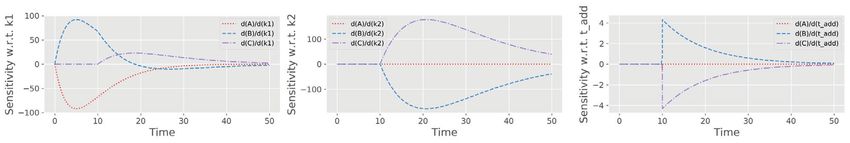
HEMMERICH et al. 7

F I G U R E 3 Essential steps of model validation supported by pyFOOMB. (A) Sensitivity analysis of the model states with respect to the
three parameters 1 , 2 and . (B) Parameter estimation using artificial experimental data with random noise (black dots with error bars)
in combination with parallelized MC sampling (red lines). The median of 125 single parameter estimations is shown in grey. (C) Uncertainty
analysis using a corner plot of the resulting empirical parameter distributions. Diagonal elements show the individual distributions as histogram
with a kernel density estimate, while off-diagonal elements indicate one-by-one comparisons of each parameter pair. The plot was generated
using the show_parameter_distributions() method of pyFOOMB’s Visualization class

8 HEMMERICH et al.

can be fixed, e.g., based on expert knowledge or litera- tion matrix, which is calculated from local sensitivities
ture data. Furthermore, model reformulation or simplifi- (see above). Besides, non-linear error propagation is
cation can be considered to reduce complexity, and here available by running a repeated parameter estimation
the model family concept (see below) allows a direct com- procedure starting from different Monte-Carlo samples
parison of different model variants. (so called “parametric bootstrapping”, Figure 3C). A
 Noteworthy, pygmo provides Python bindings to the parallelized version of this method is provided based on
pagmo2 package written in C++. It implements the asyn- the pygmo package.
chronous generalized island model [12], which allows to
run several, different algorithms cooperatively on the given
parameter estimation problem. As an inherent feature of 3.6 Result visualization
this method, an optimization run can be executed for a
given number of so-called “evolutions” and after inspec- Following parameter estimation and uncertainty analy-
tion of the results, the optimization can be continued from sis via parametric bootstrapping, (non-)linear correlations
the best solution found so far (Figure 3B). This powerful between each pair of parameters can be readily visualized
approach allows to traverse multi-modal, non-convex opti- with the method show_parameter_distributions(). In
mization landscapes. addition, results are typically inspected by visualizing the
 Currently, the maximum likelihood estimators (cover- set of model predictions according to the calculated param-
ing its classical variants least-squares and weighted-least- eter distributions. Using the compare_estimates_many()
squares) are implemented. In general, a parameter vector ˆ method, a direct comparison between measurements and
is to be found that minimizes a certain optimization (loss) repeated simulations is possible, which makes it easier to
function. For example, for the negative log-likelihood assess the validity of the model.
(NLL) function for normally distributed measurement
errors it holds:
 ∑∑∑ ( ( ))
 3.7 Implementation of model variants
 ˆ 1
 = min = ⋅ log 2 2 ˆ , , (3)
 
 2
 Usually, when starting to formulate a bioprocess model
 ( )2 there is not only one option to link a specific rate term
 , , ( ) − ˆ , , with a suitable kinetic model. Depending on how infor-
 + ( ) (3)
 ˆ , , mative the available measurements are in relation to the
 unknown kinetics, it could make sense to directly start the
Given a specific measurement ̂ , , , for each correspond- whole workflow by setting up a “model family”.
ing model response at sampling time point and replicate Following the object-oriented approach of pyFOOMB,
 , the NLL is calculated and summed up. By default, it is a model family can be easily set up based on inheritance
assumed that all measurements follow normal distribu- (Figure 4A). In principle, for each relevant part of the
tions based on mean values and corresponding standard original model additional submodels can be introduced
deviations. The log-likelihood function is constructed by declaring separate methods. In a programing context,
by pyFOOMB when starting the parameter estimation this approach is also known as “method extraction”, as
procedure. For the case that measurements are assumed the calculations in question are extracted into further
to follow other distributions, this can be specified when dedicated methods. The model family is then realized
creating the Measurement object and pyFOOMB will by building on a common model structure encoded in
take care for the definition of the correct log-likelihood the BaseModel and a set of subclasses encoding the
function. specific submodels. On a technical level, the definition of
 Noteworthy, it is not required to provide complete mea- “abstract” methods is required to enforce the individual
surement datasets, i.e., a specific replicate may contain members of the model family to implement their specific
only one measurement or even unequal data points for dif- submodel.
ferent model responses. In an extended version of the running example, the
 rhs() method of the BaseModel class now depends on the
 two additional methods get_r1() and get_r2() to sep-
3.5 Uncertainty analysis arate the calculation of rates 1 and 2 , respectively (Fig-
 ure 4B). The latter is declared as an abstract method to
An approximation of the parameters’ variance-covariance enable a family of models (ModelVariant01-03) for com-
matrix is provided by inversion of the Fisher informa- paring different rate expressions of 2 .

HEMMERICH et al. 9

F I G U R E 4 Implementation of model variants using inheritance. (A) UML class diagram for three model variants of the toy model. The
kinetic rate law for reaction 2 is set as either Mass action, Michaelis-Menten, or Michalis-Menten with product inhibition. (B) Python imple-
mentation of the base class BaseModel with the abstract method get_r2() and two example subclasses. (C) Resulting simulations comparing
the model variants

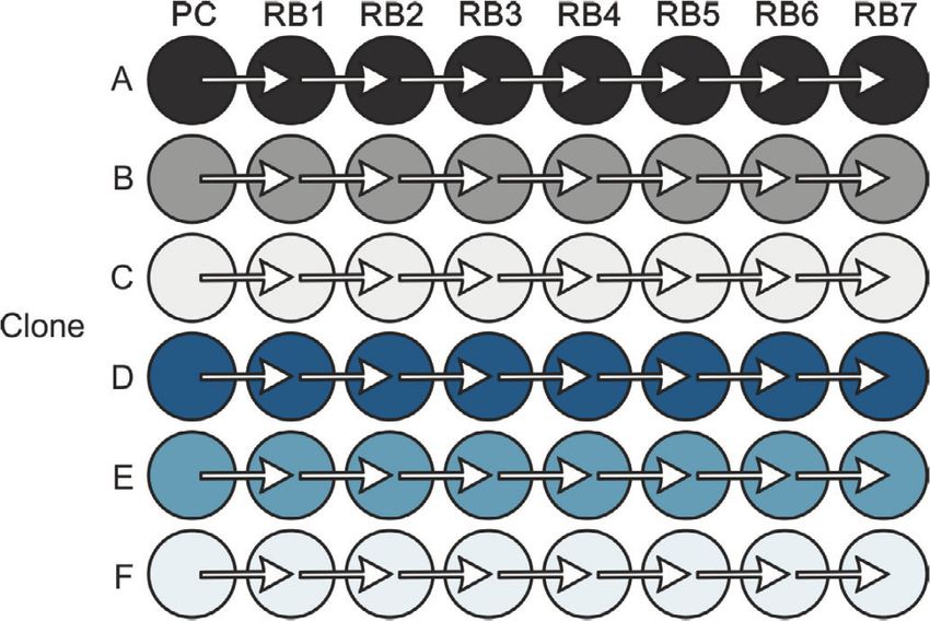
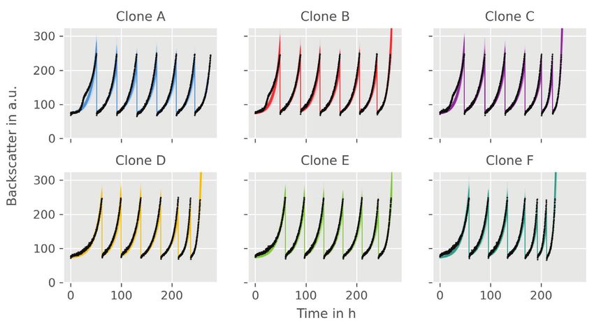
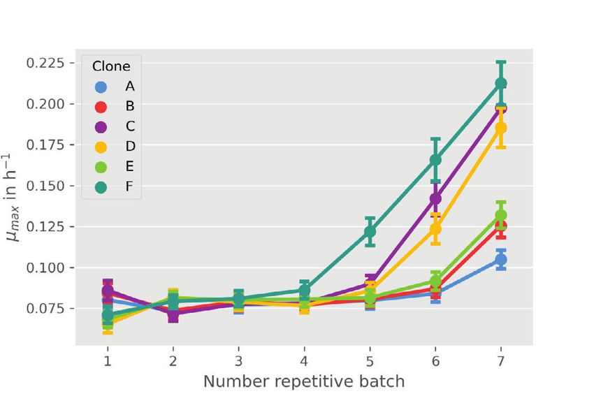
10 HEMMERICH et al.

 In the following sections two different applications inoculation procedure within the experiment was the same
examples will be presented that apply the introduced for all, initial biomass concentration 0 and dilution factor
modeling workflow of pyFOOMB. dil are considered as global parameters.

4 APPLICATION EXAMPLE I: 4.2 Parameter estimation and
SMALL-SCALE REPETITIVE BATCH uncertainty analysis
OPERATION
 In total, model parameters for six clones are esti-
In the first example workflow specific growth rates within mated, which form six replicates in the context of
an Adaptive Laboratory Evolution (ALE) process are pyFOOMBs modeling structure. For each clone, seven
determined. ALE processes utilize the natural ability of maximum growth rates are to be determined, plus 0 ,
microorganisms to adapt to new environments to improve dil , and 0 as global parameters, thus 44 parameters
certain strain characteristics, such as growth on a specific in total. Parallelized MC sampling was used to obtain
carbon source. distributions for all parameters. Results are shown in
 Here, a Corynebacterium glutamicum strain which Figure 5C and D.
was able to slowly ( max < 0.10 h-1 ) utilize d-xylose, The estimated backscatter signals follow the actual data
was cultivated repeatedly in defined medium containing closely, resulting in narrow distributions for the parame-
d-xylose as sole carbon and energy source. The cultivation ters of interest, the individual max values for each clone
was done in an automated and miniaturized manner, and repetitive batch. For example, clone F starts with
delivering a biomass-related optical signal, “backscatter”, growth rates of 0.071 ± 0.005 h-1 to 0.086 ± 0.005 h-1 for the
with a high temporal resolution. This signal was used first four batches. In the fifth batch, a notable raise in max-
to automatically start a new batch from the previous imum growth rate to 0.122 ± 0.008 h-1 is visible, indicating
one, as soon as a backscatter threshold was reached. one or more beneficial mutation events. Finally, clone F
The threshold was deliberately chosen to be in the mid- reaches a growth rate of 0.212 ± 0.013 h-1 . Overall, the esti-
exponential phase, where no substrate limitation was to mated growth rates are in good agreement with findings
be expected. Six individual clones were cultivated over from the original paper.
one preculture and seven repetitive batches, as shown in In another style of ALE experiment, which is not
Figure 5A. subject in this study, a subpopulation of cells with
 beneficial mutations was enriched, yielding strain
 WMB2 , which is analyzed in the second application
4.1 Model development example.

In order to keep the number of parameters and computa-
tion times as low as possible, a rather simple bioprocess 5 APPLICATION EXAMPLE II:
model as shown in Figure 5B was employed. LAB-SCALE PARALLEL BATCH
 Growth is determined solely by the growth rate OPERATION
 . Substrate limitations are not taken into account,
since the experimental design (see above) should avoid In this example workflow some KPIs of an engineered
these sufficiently. Biomass is not measured directly, microbial strain cultivated in a bioreactor under batch
instead, backscatter is introduced to the model via an operation are determined. Often, such KPIs represent
ObservationFunction. This function describes a linear process quantities that are not directly measurable (e.g.,
relationship between backscatter and biomass and takes specific rates for substrate uptake, biomass and product
the blank value 0 of the signal into account. A rela- formation) and therefore have to be estimated using a
tive measurement error for the backscatter signal of 5% is model-based approach.
assumed based on expert knowledge. The model describes The data originates from two independent cultiva-
the whole ALE process for each clone, not an individual tion experiments with the evolved C. glutamicum strain
batch. Therefore, state events are used to trigger a state WMB2 as introduced before [13]. Following successful
change of , where is multiplied by a dilution factor adaptive laboratory evolution this strain has now improved
 dil . Additionally, the maximum growth rate parameter is properties for utilizing d-xylose as sole carbon and energy
switched for each repetitive batch. As a result, an individ- source for biomass growth. At the same time the strain pro-
ual max for each repetitive batch and each clone is gained. duces significant amounts of d-xylonate, a direct oxidation
Since initial inoculation of the different clones and the product of d-xylose.

HEMMERICH et al. 11

F I G U R E 5 Modeling and analysis of small-scale repetitive batch processes. (A) Experimental layout for fully automated repetitive batch
operation in microtiter plates (taken from [13]. Each cycle was started from six independent clones followed by seven consecutive batches. (B)
ODE model for describing the biomass dynamics including state events for multiple sampling and growth rate estimation. (C) Time course of
online backscatter data (black dots) and corresponding model fits (straight colored lines). (D) Evolution of maximum specific growth rates in
each cycle. Mean values and standard deviations were estimated by parallelized MC sampling ( = 200)

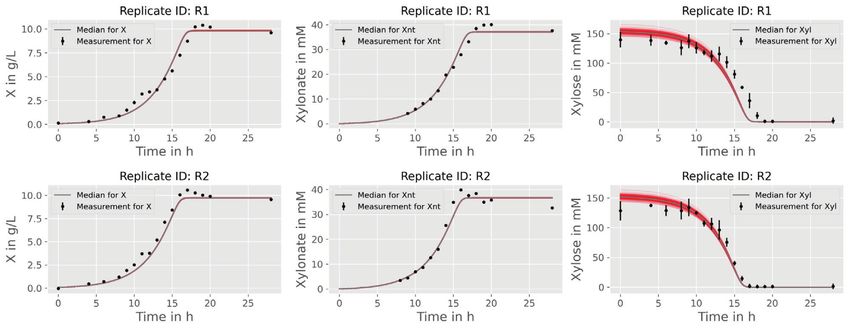
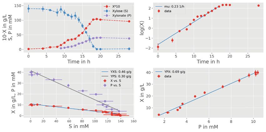
12 HEMMERICH et al.

5.1 Explorative data analysis and model T A B L E 2 Estimated parameter values of the bioprocess model
development applying parallelized MC sampling
 Median (16, 84
Before implementing a suitable bioprocess model with Parameter Property Unit percentile)
pyFOOMB, the data from one replicate bioreactor cultiva- global g L-1 1.86 (1.83–1.89)
tion is visualized and used for explorative data analysis. max global h -1
 0.33 (0.33–0.33)
In Figure 6A, the time courses of biomass ( ), d-xylose P/S global g g -1 0.80 (0.68–0.99)
( ), and d-xylonate ( ) are presented in one subplot. It can P/X global g g -1
 0.63 (0.63–0.63)
be seen that biomass formation stops with depletion of d- X/S global g g -1 0.63 (0.58–0.69)
xylose and, thus, modeling the cell population growth by a 0,R1 local g L -1
 23.04 (22.76–23.36)
classical Monod kinetic is reasonable (Figure 6B). The for- 0,R2 local g L-1 22.78 (22.50–23.09)
mation of d-xylonate is also strictly growth-coupled, lead-
 0,R1 local g L -1
 0.070 (0.070–0.071)
ing to a simple rate equation with the yield coefficient P/X
 0,R2 local g L-1 0.088 (0.088–0.088)
as proportionality factor. Finally, the d-xylose uptake rate
equals the combined carbon fluxes into biomass and d-
xylonate, which are related to the yield coefficients X/S
 The pair-wise comparison of parameter distributions
and P/S respectively.
 shown in Figure 7B reveals a distinct non-linear corre-
 The time courses of substrate and product are measured
 lation between the yield coefficients P/S and X/S . This
in molar concentrations, while the bioprocess model is
 effect is expected due to the formulation of the biomass-
formulated using mass concentrations of the respective
 specific substrate consumption rate (Figure 6B). Equal
species. The mappings are realized by defining correspond-
 values for can be derived for different combination of
ing observation functions (Figure 6C).
 substrate conversion rates into biomass and product, and
 Finally, the strain-specific parameters like max
 the yield coefficients are the corresponding scaling factors.
and X/S are defined as global parameters, while
 The latter is also the reason why the estimated yield coef-
experiment-specific parameters (ICs for biomass 
 ficients are significantly higher as compared to the explo-
and substrate ) are defined as local parameters since
 rative data analysis, which does not allow this separation
the cultivation media and inoculation material were
 and therefore leads to false-to-low predictions (Table 2 and
prepared individually for each reactor. Please note, even
 Figure 6A).
this very simple process model now already contains
 Finally, the estimated biomass yield X/S for d-xylose is
eight model parameters (i.e., three ICs and five kinetic
 close to the value reported for the wild-type strain growing
parameters) that have to be estimated from the given
 on d-glucose, i.e., 0.63 [CI: 0.58–0.69] vs. 0.60 ± 0.04 g g -1
measurements.
 [16]. This indicates a comparable efficiency of C. glutam-
 icum WMB2 in utilizing d-xylose for biomass growth.

5.2 Parameter estimation and
uncertainty analysis 6 CONCLUSIONS

In order to facilitate the parameter estimation problem, The pyFOOMB package provides straight-forward access
good initial guesses for all parameter values are important. to the formulation of bioprocess models in a programatic
First approximations for max as well as all yield coeffi- and object-oriented manner. Based on the powerful, yet
cients can be derived by following ordinary and orthogo- beginner-friendly Python programing language, the pack-
nal distance regression analysis on the raw data assuming age addresses a wide range of users to implement mod-
linear relationships (Figure 6A). For Python, correspond- els with growing complexity. For example, by employing
ing methods are available from the NumPy [14] and SciPy event methods, pyFOOMB supports the modeling of dis-
[15] packages. crete behaviors in process quantities, which is an impor-
 From the obtained initial guesses corresponding param- tant feature for the simulation and optimization of fed-
eter bounds are fixed to run a parallel parameter estimation batch processes. The concept of model replicates and
procedure (Figure 7A). As a result, a first set of best-fitting definition of local and global parameters mirrors the iter-
parameter values is obtained from which new bounds can ative nature of data generation from cycles of experiment
be derived for the subsequent uncertainty analysis using design, execution and evaluation. Moreover, seamless inte-
again parallelized MC sampling. Corresponding results are gration with existing and future Python packages for scien-
summarized in Table 2. tific computing is greatly facilitated.

HEMMERICH et al. 13

F I G U R E 6 Modeling of lab-scale batch processes. (A) Explorative data analysis for one replicate culture. Concentrations for biomass,
d-xylose and d-xylonate are denoted by symbols , , and , respectively. Following linear regression analysis first estimates for the model
parameters X/S , P/S and P/X can be derived (for later comparison values are transformed to mass-based units). (B) ODE model using classical
rate equations. (C) Formulation of specific observation functions to map the state variables to the measurements. Here simple transformations
from measured molar concentrations to simulated mass concentrations are performed

14 HEMMERICH et al.

F I G U R E 7 Results from repeated parameter estimation using parallelized MC sampling ( = 200). (A) Comparison of model predictions
with experimental data. (B) Uncertainty analysis using a corner plot of the resulting empirical parameter distributions. For the sake of brevity,
only the global model parameters are shown

HEMMERICH et al. 15

 In summary, pyFOOMB is an ideal tool for model-based 3. Fröhlich, F., Theis, F. J., Rädler, J. O., Hasenauer, J., Parameter
integration and analysis of data from classical lab-scale estimation for dynamical systems with discrete events and logi-
experiments to state-of-the-art high-throughput biopro- cal operations. Bioinformatics 2017, 33, 1049–1056.
 4. Fröhlich, F., Kaltenbacher, B., Theis, F. J., Hasenauer, J., Scal-
cess screening approaches.
 able parameter estimation for genome-scale biochemical reac-
 tion networks. PLoS Comput. Biol. 2017, 13, e1005331.
 5. Hoops, S., Sahle, S., Gauges, R., Lee, C., et al., Copasi - a complex
7 AVAILABILITY pathway simulator. Bioinformatics 2006, 22, 3067–3074.
 6. Welsh, C. M., Fullard, N., Proctor, C. J., Martinez-Guimera, A.,
The source code for the pyFOOMB package is freely avail- et al., Pycotools: a python toolbox for copasi. Bioinformatics
able at github.com/MicroPhen/pyFOOMB. It is published 2018, 34, 3702–3710.
under the MIT license. Currently, its compatibility is tested 7. Nikolić, D. D., Dae tools: equation-based object-oriented mod-
 elling, simulation and optimisation software. PeerJ Computer
with Python 3.7 and 3.8, for Ubuntu and Windows operat-
 Sci. 2016, 2, e54.
ing systems. The use of pyFOOMB within a conda envi- 8. Nikolić, D. D., Parallelisation of equation-based simulation pro-
ronment is recommended, since the most recent versions grams on heterogeneous computing systems. PeerJ Computer
of important dependencies are maintained at the conda- Sci. 2018, 4, e160.
forge channel. 9. Hindmarsh, A. C., Brown, P. N., Grant, K. E., Lee, S. L., et al.,
 Sundials: Suite of nonlinear and differential/algebraic equation
AC K N OW L E D G E M E N T S solvers. ACM Trans. Math. Softw. 2005, 31, 363–396.
 10. Andersson, C., Führer, C., Åkesson, J., Assimulo: a unified
This work was partly funded by the German Federal
 framework for ode solvers. Math. Comput. Simul. 2015, 116, 26–
Ministry of Education and Research (BMBF, projects:
 43.
“Digitalization in Industrial Biotechnology”, grant no. 11. Biscani, F., Izzo, D., A parallel global multiobjective frame-
031B0463 and “BioökonomieREVIER_INNO: Entwick- work for optimization: pagmo. J. Open Source Softw. 2020, 5,
lung der Modellregion BioökonomieREVIER Rheinland”, 2338.
grant no. 031B0918A). Further funding was received from 12. de Vega, F. F., Pérez, J. I. H., Lanchares, J. Parallel Architectures
the Bioeconomy Science Center (BioSC, Focus FUND and Bioinspired Algorithms, Springer, New York 2012.
project “HyImPAct - Hybrid processes for important pre- 13. Radek, A., Tenhaef, N., Müller, M. F., Brüsseler, C., et al., Minia-
 turized and automated adaptive laboratory evolution: evolving,
cursor and active pharmaceutical ingredients”, grant no.
 Corynebacterium glutamicum towards an improved d-xylose uti-
313/323-400-00213).
 lization. Bioresource Technol. 2017, 245, 1377–1385.
 14. Harris, C. R., Millman, K. J., van der Walt, S. J., Gommers, R.,
CONFLICT OF INTEREST et al., Array programming with numpy. Nature 2020, 585, 357–
The authors have no conflict of interest to declare. 362.
 15. Virtanen, P., Gommers, R., Oliphant, T. E., Haberland, M., et al.,
ORCID Scipy 1.0: fundamental algorithms for scientific computing in
Johannes Hemmerich https://orcid.org/0000-0002- python. Nat. Methods 2020, 17, 261–272.
 16. Baumgart, M., Unthan, S., Kloß, R., Radek, A., et al., Corynebac-
9786-6315
 terium glutamicum chassis C1*: building and testing a novel plat-
Niklas Tenhaef https://orcid.org/0000-0002-9375-4156 form host for synthetic biology and industrial biotechnology.
Wolfgang Wiechert https://orcid.org/0000-0001-8501- ACS Synth. Biol. 2018, 7, 132–144.
0694
Stephan Noack https://orcid.org/0000-0001-9784-3626

REFERENCES
 How to cite this article: Hemmerich J, Tenhaef
 1. Balsa-Canto, E., Henriques, D., Gábor, A., Banga, J. R., Amigo2,
 N, Wiechert W, Noack S. pyFOOMB: Python
 a toolbox for dynamic modeling, optimization and control in sys-
 tems biology. Bioinformatics 2016, 32, 3357–3359. framework for object oriented modeling of
 2. Tsiantis, N., Balsa-Canto, E., Banga, J. R., Optimality and identi- bioprocesses. Eng Life Sci. 2020;1–16.
 fication of dynamic models in systems biology: an inverse opti- https://doi.org/10.1002/elsc.202000088
 mal control framework. Bioinformatics 2018, 34, 2433–2440.

16 HEMMERICH et al.

APPENDIX A: NOTEBOOK EXAMPLES

TA B L E A 1 Jupyter notebook examples provided with the pyFOOMB package
 # Title Topic
 1 Modeling Demonstrates basic usage of the pyFOOMB package based on a simple toy mass-action kinetic, i.e. how to
 implement the right-hand-side of the resulting equation system and how to run and visualize
 simulations. The concept of model replicates is introduced and resulting effects are visualized.
 2 Events The previous model is extended by events, which are timepoints where the model behavior can be
 changed safely without interfering with the multistep logic of the ODE integrator. Shows how to use
 different parameter values before and after an event, as well as how to manipulate the model state
 values upon reaching an event.
 3 Observation Introduces observation functions that map a model state to an observation, according to a specific,
 functions parametrized function.
 4 Parameter Describes one of the major functionalities of the pyFOOMB package. Parameter values of an implemented
 estimation model are estimated based on (artificial) noisy data. The presented methods use algorithms from
 Scipy’s optimize module. Besides approximation of uncertainties for estimated parameters based on
 Fisher information matrix, Monte-Carlo sampling is introduced as method for non-linear error
 propagation. Suitable visualization methods are used for interpretation of results.
 5 Sensitivities Shows how to calculate local sensitivities with subsequent visualization.
 6 Bioprocess Implements several example bioprocess models, serving as starting point for implementation of
 models user-specific ones.
 7 Fed-batch Demonstrates the implementation of fed-batch bioprocess models at various complexities. Shows how to
 models use the models to derive further performance indicators such as maximum yield and productivity and
 how to get these from a model parameters’ search. In addition, the formulation of the corresponding
 optimization problem is presented.
 8 Measurement Loading measurement data from spreadsheet files with subsequent creation of “Measurement” objects,
 data focusing on three use cases that are based on: 1) Individual time vectors of varying lengths, with a
 shared time vector; 2) A shared time vector but missing data points for several measurements, and 3)
 Multi-replicate experiments with a shared time vector but missing data points.
 9 Parallel Introduces PPE and the concept of continuation of an estimation job.
 parameter
 estimation
 (PPE)
 10 PPE - Optimizer Compares different optimization algorithms for PPE of a simple bioprocess model utilizing artifical noisy
 comparison data. Comparison is based on runtimes and achieved losses for the given optimization problem.
 11 PPE - Hyperpa- Demonstrates how different parameter settings of the “de1220” and “compass_search” algorithms affect
 rameter runtime and quality of the model calibration outcome.
 adjustment
 12 PPE - Monte Introduces the application of PPE for Monte-Carlo sampling as method for non-linear error propagation.
 Carlo
 sampling
 13 PPE - Monte In addition to the previous examples, the possibility to apply further constraints (beyond simple box
 Carlo bounds for parameters) is demonstrated.
 Sampling
 14 Tracking Shows how specific rates can be derived and visualized as time-dependent performance indicators.
 specific rates
 during
 integration
 15 Non-negative For enforcing non-negative state values, events can be employed. Without, state values can take very
 states small but negative numbers due to the operation mode of the integrator, which treats those values
 internally as zero (depending on the specified tolerances).