Dimensionality Reduction for Dynamic Movement Primitives and Application to Bimanual Manipulation of Clothes - UPC
←
→
Page content transcription
If your browser does not render page correctly, please read the page content below
Dimensionality Reduction for Dynamic Movement Primitives and
             Application to Bimanual Manipulation of Clothes
                         Adrià Colomé, Member, IEEE, and Carme Torras,Senior Member, IEEE

   Abstract— Dynamic Movement Primitives (DMPs) are nowa-                   domain by learning trajectories [2], [3], but it can also be
days widely used as movement parametrization for learning                   carried out in the force domain [4], [5], [6].
robot trajectories, because of their linearity in the parameters,              A training data set is often used in order to fit a relation be-
rescaling robustness and continuity. However, when learning
a movement with DMPs, a very large number of Gaussian                       tween an input (experiment conditions) and an output (a good
approximations needs to be performed. Adding them up for all                behavior of the robot). This fitting, which can use different
joints yields too many parameters to be explored when using                 regression models such as Gaussian Mixture Models (GMM)
Reinforcement Learning (RL), thus requiring a prohibitive                   [7], is then adapted to the environmental conditions in order
number of experiments/simulations to converge to a solution                 to modify the robot’s behavior [8]. However, reproducing
with a (locally or globally) optimal reward. In this paper
we address the process of simultaneously learning a DMP-                    the demonstrated behavior and adapting it to new situations
characterized robot motion and its underlying joint couplings               does not always solve a task optimally, thus Reinforcement
through linear Dimensionality Reduction (DR), which will                    Learning (RL) is also being used, where the solution learned
provide valuable qualitative information leading to a reduced               from a demonstration improves through exploratory trial-
and intuitive algebraic description of such motion. The results             and-error. RL is capable of finding better solutions than the
in the experimental section show that not only can we effectively
perform DR on DMPs while learning, but we can also obtain                   one demonstrated to the robot.
better learning curves, as well as additional information about
each motion: linear mappings relating joint values and some
latent variables.

                        I. I NTRODUCTION
   Motion learning by a robot may be implemented in a
similar way to how humans learn to move. An initial
coarse movement is learned from a demonstration and then
rehearsed, performing some local exploration to adapt and
possibly improve the motion.
   We humans activate in a coordinated manner those mus-
cles that we cannot control individually [1], generating
coupled motions of our articulations that gracefully move our
skeletons. Such muscle synergies lead to a drastic reduction
in the number of degrees of freedom, which allows humans
to learn and easily remember a wide variety of motions.
   For most current robots, the relation between actuators                  Fig. 1: Two robotic arms coordinating their motions to fold a polo shirt.
and joints is more direct than in humans, usually linear, as
in Barrett’s WAM robot.                                                        These motor/motion behaviors are usually represented
   Learning robotic skills is a difficult problem that can be               with Movement Primitives (MPs), parameterized trajectories
addressed in several ways. The most common approach is                      for a robot that can be expressed in different ways, such as
Learning from Demonstration (LfD), in which the robot is                    splines, Gaussian mixtures [9], probability distributions [10]
shown an initial way of solving a task, and then tries to                   or others. A desired trajectory is represented by fitting certain
reproduce, improve and/or adapt it to variable conditions.                  parameters, which can then be used to improve or change it,
The learning of tasks is usually performed in the kinematic                 while a proper control (a computed torque control [11], for
                                                                            example) tracks this reference signal.
   This work was partially developed in the context of the Advanced Grant      Among all MPs, the most used ones are Dynamic Move-
CLOTHILDE (”CLOTH manIpulation Learning from DEmonstrations”),              ment Primitives (DMPs) [12], [13], which characterize a
which has received funding from the European Research Council (ERC)         movement or trajectory by means of a second-order dy-
under the European Union’s Horizon 2020 research and innovation pro-
gramme (grant agreement No 741930). This work is also partially funded      namical system. The DMP representation of trajectories has
by CSIC projects MANIPlus (201350E102) and TextilRob (201550E028),          good scaling properties wrt. trajectory time and initial/ending
and Chist-Era Project I-DRESS (PCIN-2015-147).                              positions, has an intuitive behavior, does not have an explicit
   The authors are with the Institut de Robòtica i Informàtica Indus-
trial (CSIC-UPC), Llorens Artigas 4-6, 08028 Barcelona, Spain. E-mails:     time dependence and is linear in the parameters, among other
[acolome,torras]@iri.upc.edu                                                advantages [12]. For these reasons, DMPs are being widely
used with Policy Search (PS) RL [14], [15], [16], where           with the tradeoff between exploitation and exploration in
the problem of finding the best policy (i.e., MP parame-          the parameter space to obtain a compact and descriptive
ters) becomes a case of stochastic optimization. Such PS          projection matrix which helps the RL algorithm to converge
methods can be gradient-based [16], based on expectation-         faster to a (possibly) better solution. Additionally, Policy
maximization approaches [15], can also use information-           Search approaches in robotics usually have few sample
theoretic approaches like Relative Entropy Policy Search          experiments to update their policy. This results in policy
(REPS) [17], [18] or be based on optimal control theory,          updates where there are less samples than parameters, thus
as for the case of Policy Improvement with Path Integrals         providing solutions with exploration covariance matrices that
(PI2) [19], [20], [21]. All these types of PS try to optimize     are rank-deficient (note that a covariance matrix obtained
the policy parameters θ, which in our case will include the       by linear combination of samples can’t have a higher rank
DMPs’ weights, so that an expected reward J(θ) is maximal,        than the number of samples itself). These matrices are
i.e., θ ∗ = argmaxθ J(θ). After each trajectory reproduction,     usually then regularized by adding a small value to the
namely rollout, the reward/cost function is evaluated and,        diagonal so the matrix remains invertible. However, this
after a certain number of rollouts, used to search for a set      procedure is a greedy approach, since the unknown subspace
of parameters that improves the performance over the initial      of the parameter space is given a residual exploration value.
movement.                                                         Therefore, performing DR in the parameter space results
   These ideas have resulted in algorithms that require several   in the elimination of unexplored space. On the contrary,
rollouts to find a proper policy update. In addition, to have     if such DR is performed in the DoF space, the number of
a good fitting of the initial movement, many parameters are       samples is larger than the DoF of the robot and, therefore,
required, while we want to have few in order to reduce the        the elimination of one degree of freedom of the robot (or a
dimensionality of the optimization problem. When applying         linear combination of them) will not affect such unexplored
learning algorithms using DMPs, several aspects must be           space, but rather a subspace of the DoF of the robot that has
taken into account:                                               a negligible impact on the outcome of the task.
                                                                     Other works [23], [24], [25] proposed dimensionality
  •   Model availability. RL can be performed through sim-
                                                                  reduction techniques for MP representations. In our previ-
      ulation or with a real robot. The first case is more
                                                                  ous work [26], we showed how an iterative dimensionality
      practical when a good simulator of the robot and
                                                                  reduction applied to DMPs, using policy reward evaluations
      its environment is available. However, in the case of
                                                                  to weight such DR could improve the learning of a task, and
      manipulation of non-rigid objects or, more generally,
                                                                  [27] used weighted maximum likelihood estimations to fit a
      when accurate models are not available, reducing the
                                                                  linear projection model for MPs.
      number of parameters and rollouts is critical. Therefore,
                                                                     In this paper, our previous work [26] is extended with
      although model-free approaches like deep reinforcement
                                                                  a better reparametrization after DR, and generalized by
      learning [22] could be applied in this case, they require
                                                                  segmenting a trajectory using more than a single projection
      large resources to successfully learn motion.
                                                                  matrix. The more systematic experimentation in three set-
  •   Exploration constraints. Certain exploration values
                                                                  tings shows their clear benefits when used for reinforcement
      might result in dangerous motion of the real robot, such
                                                                  learning. After introducing some preliminaries in Section
      as strong oscillations and abrupt acceleration changes.
                                                                  II, we will present the alternatives to reduce the parameter
      Moreover, certain tasks may not depend on all the
                                                                  dimensionality of the DMP characterization in Section III,
      Degrees of Freedom (DoF) of the robot, meaning that
                                                                  focusing on the robot’s DoF. Then, experimental results with
      the RL algorithm used might be exploring motions that
                                                                  a simulated planar robot, a single 7-DoF WAM robot, and
      are irrelevant to the task, as we will see later.
                                                                  a bimanual task performed by two WAM robots will be
  •   Parameter dimensionality. Complex robots still re-
                                                                  discussed in Section IV, followed by conclusions and future
      quire many parameters for a proper trajectory repre-
                                                                  work prospects in Section V.
      sentation. The number of parameters needed strongly
      depends on the trajectory length or speed. In a 7-DoF                           II. P RELIMINARIES
      robot following a long 20-second trajectory, the use          Throughout this work, we will be using DMPs as motion
      of more than 20 Gaussian kernels per joint might be         representation and REPS as PS algorithm. For clarity of
      necessary, thus having at least 140 parameters in total.    presentation, we firstly introduce the basic concepts we will
      A higher number of parameters will usually allow for        be using throughout this work.
      a better fitting of the initial motion characterization,
      but performing exploration for learning with such a         A. Dynamic Movement Primitives
      high dimensional space will result in a slower learning.      In order to encode robot trajectories, DMPs are widely
      Therefore, there is a tradeoff between better exploita-     used because of their adaptability. DMPs determine the
      tion (many parameters) and efficient exploration (fewer     robot commands in terms of acceleration with the following
      parameters).                                                equation:
For these reasons, performing Dimensionality Reduction                      ÿ/τ 2 = αz (βz (G − y) − ẏ/τ ) + f (x)
                                                                                                                            (1)
(DR) on the DMPs’ DoF is an effective way of dealing                                     f (x) = ΨT ω,
where y is the joint position vector, G the goal/ending joint         tasks policies which could result in dangerous robot motion.
position, τ a time constant, x is a transformation of time            Formally:
verifying ẋ = −αx x/τ . In addition, ω is the parameter                             π ∗ = argmaxπ π(ω)R(ω)dω
                                                                                                    R
vector of size dNf , Nf being the number of Gaussian kernels
                                                                                      s.t. KL ≥ π(ω)log π(ω)
                                                                                                 R
used for each of the d DoF. The parameters ω j , j = 1..d                                         R         q(ω) dω            (3)
fitting each joint behavior from an initial move are appended                                 1 = π(ω)dω
to obtain ω = [ω 1 ; ...; ω d ], and then multiplied by a Gaussian    where ω are the parameters of a trajectory, R(ω) their
weights matrix Ψ = Id ⊗ g(x), ⊗ being the Kronecker                   reward, and π(ω) is the probability, according to the policy
product, with the basis functions g(x) defined as:                    π, of having such parameters. For DMPs, the policy π will
                                                                      be represented by µω and Σω , generating sample trajectories
                         φi (x)
              gi (x) = P          x, i = 1..Nf ,          (2)         ω.
                         j φj (x)                                       Solving this constrained optimization problem provides a

where φi (x) = exp −0.5(x − ci )2 /di , and ci , di represent         solution of the form
the fixed center and width of the ith Gaussian.                                            π ∗ ∝ q(ω)exp(R(ω)/η),                          (4)
   With this motion representation, the robot can be taught
a demonstration movement, to obtain the weights ω of                  where η is the solution of a dual function (see [17] for
the motion by using least squares or maximum likelihood               details on this derivation). Having the value of η and the
techniques on each joint j separately, with the values of f           rewards, the exponential part in Eq. (4) acts as a weight
isolated from Eq. (1).                                                to use with the trajectory samples ω k in order to obtain
                                                                      the new policy, usually with a Gaussian weighted maximum
B. Learning an initial motion from demonstration                      likelihood estimation.
                                                                         Table I shows a list of the parameters and variables
   A robot can be taught an initial motion through kines-             used throughout this paper; those related to the coordination
thetic teaching. However, in some cases, the robot might              matrix will be introduced in the following section.
need to learn an initial trajectory distribution from a set of
demonstrations. In that case, similar trajectories need to be                     TABLE I: Parameters and variables
aligned in time. In the case of a single-demonstration, the
                                                                        θ = {Ω, µω Σω }      DMP parameters
user has to provide an arbitrary initial covariance matrix Σω           Ω                    Coordination matrix
for the weights distribution with a magnitude providing as              ω ∼ N (µω , Σω )     DMP weights with mean and covariance
much exploration as possible while keeping robot behavior               αz , βz , αx , τ     DMP fixed parameters
                                                                        d, r                 Robot’s DOF and reduced dimensionality
stable and safe. In the case of several demonstrations, we              Nf                   Gaussian basis functions used per DoF
can sample from the parameter distribution, increasing the              k, Nk                Rollout index and number of rollouts per
covariance values depending on how local we want our                                         policy update
                                                                        t, Nt                Time index and number of timesteps
policy search to be.                                                    s, Ns                Coordination matrix index and number of
   Given a set of taught trajectories τ1 , ..., τNk , we can obtain                             coordination matrices
the DMP weights for each one and fit a normal distribution              y, x                 Robot’s joint position vector and end effector’s
                                                                                                Cartesian pose
ω ∼ N (µω , Σω ), where Σω encodes the time-dependent
variability of the robot trajectory at the acceleration level.
To reproduce one of the trajectories from the distribution,                             III. DMP COORDINATION
the parameter distribution can be sampled, or tracked with               In this section, we will describe how to efficiently obtain
a proper controller that matches the joint time-varying vari-         the joint couplings associated to each task during the learning
ance, as in [28].                                                     process, in order to both reduce the dimensionality of a
   This DMP representation of a demonstrated motion will              problem, as well as obtaining a linear mapping describ-
then be used to initialize a RL process, so that after a              ing a task. In [30], a coordination framework for DMPs
certain number of reproductions of the trajectory (rollouts),         was presented, where a robot’s movement primitives were
a cost/reward function will be evaluated for each of those            coupled through a coordination matrix, which was learned
trajectories, and a suitable RL algorithm will provide new            with an RL algorithm. Kormushev et al. [31] worked in a
parameters that represent a similar trajectory, with a higher         similar direction, using square matrices to couple d primitives
expected reward.                                                      represented as attractor points in the task space domain.
                                                                         We now propose to use a not necessarily square coordina-
C. Policy search                                                      tion matrix in order to decrease the number of actuated DoF
   Along this work, we will be using Relative Entropy Policy          and thus reduce the number of parameters. To this purpose,
Search (REPS) as PS algorithm. REPS [17], [18] finds the              in Eq. (1) we can take:
policy that maximizes the expected reward of a robotic
                                                                                              f (xt ) = ΩΨTt ω,                            (5)
task, subject to the constraint of a bound on the Kullback-
Leibler Divergence [29] of the new policy with respect to             for each timestep t, Ω being a (d × r) matrix, with r ≤ d
the previous policy q(ω), to avoid large changes in robotic           a reduced dimensionality, ΨTt = Ir ⊗ g, similarly as in the
previous section, and ω is an (rNf )-dimensional vector of be the first r columns of Upca = [u1 , ..., ur , ..., ud ], with
motion parameters. Note that this representation is equivalent associated singular values σ1 > σ2 > ... > σd and use
to having r movement primitives encoding the d-dimensional
Ω = [u1 , ..., ur ] (8)
acceleration command vector f (x). Intuitively, the columns
of Ω represent the couplings between the robot’s DoF. as coordination matrix in Eq. (5), having a reduced set
The DR reduction in Eq. (5) is preferable to a DR on of DoF of dimension r, which activate the robot joints
the DMP parameters themselves for numerical reasons. If (dimension d), minimizing the error in the reprojection e =
such DR would be performed as f (xt ) = ΨTt Ω̂ω, then Ω̂ kF−Ω·Σ·Vpca T
k2F rob , with Σ the part of Σpca corresponding
would be a high-dimensional matrix but, more importantly, to the first r singular values.
the number of rollouts per policy update performed in PS Note that this dimensionality reduction does not take any
algorithms would determine the maximum dimension of the reward/cost function into consideration, so an alternative
explored space as a subspace of the parameter space, leaving would be to start with a full-rank coordination matrix and
the rest of such parameter space with zero value or a small progressively reduce its dimension, according to the costs or
regularization value at most. In other words, performing DR rewards of the rollouts. In the next section, we will explain
in the parameter space requires Nf times more rollouts per the methodology to update such coordination matrix while
update to provide full information than performing such DR also reducing its dimensionality, if necessary.
in the joint space.
B. Reward-based Coordination Matrix Update (CMU)
In order to learn the coordination matrix Ω, we need an
initial guess and also an algorithm to update it and eliminate In order to tune the coordination matrix once initialized
unnecessary degrees of freedom from the DMP, according as described in Section III-A, we assume we have performed
to the reward/cost obtained. Within this representation, we Nk reproductions of motion, namely rollouts, obtaining an
(j),k
can assume that the probability of having certain excitation excitation function ft , for each rollout k = 1..Nk ,
values ft = f (xt ) at a timestep given the weights ω is timestep t = 1..Nt , and DoF j = 1..d. Now having eval-
p(ft |ω) ∼ N (ΩΨTt ω, Σf ), Σf being the system noise. Thus, uated each of the trajectories performed with a cost/reward
if ω ∼ N (µω , Σω ), the probability of ft is: function, we can also associate a relative weight Ptk to each
rollout and timestep as it is done in policy search algorithms
p(ft ) = N (ΩΨTt µω , Σf + ΩΨTt Σω Ψt ΩT ). (6) such as PI2 or REPS. We can then obtain a new d×Nt matrix
Fco with the excitation function on all timesteps defined as:
Along this section we will firstly present the initialization Nk N
of such coordination matrices in Section III-A, and how they P (1),k k Pk (1),k k
k=1 1f P 1 ... f Nt P Nt
can be updated with a reward-aware procedure in Section III- k=1
new
B. Additionally, Section III-C presents ways of eliminating Fco = ... ... ,
(9)
robot DoF irrelevant for a certain task, and in Section III- NPk (d),k k N
Pk (d),k k
f1 P1 ... fNt PNt
E, we present a multiple coordination matrix framework to k=1 k=1
segment a trajectory so as to use more than one projection which contains information of the excitation functions,
matrix. Finally, we consider some numerical issues in Section weighted by their relative importance according to the rollout
III-F and a summary in Section III-G. result. A new coordination matrix Ω can be obtained by
means of PCA. However, when changing the coordination
A. Obtaining an initial coordination matrix with PCA matrix, we then need to reevaluate the parameters {µω , Σω }
In this section, we will explain how to obtain the coordina- to make the trajectory representation fit the same trajectory.
tion motion matrices while learning a robotic task, and how To this end, given the old distribution (represented with a hat)
to update them. A proper initialization for the coordination and the one with the new coordination matrix, the excitation
matrix Ω is to perform a Principal Component Analysis functions distributions, excluding the system noise, are
(PCA) over the demonstrated values of f (see Eq(1)). Taking T T T
the matrix F of all timesteps ft in Eq. (5), of size (d × Nt ), f̂t ∼ N (Ω̂Ψ̂t µ̂ω , Ω̂Ψ̂t Σˆω Ψ̂t Ω̂ ) (10)
for the d degrees of freedom and Nt timesteps as: ft ∼ N (ΩΨTt µω , ΩΨTt Σω Ψt ΩT ). (11)
(1) (1)
(1) (1)
fde (x0 ) − f de ... fde (xNt ) − f de We then represent the trajectories as a single probability
F=
... ... , (7)
distribution over f using (6):
(d) (d) (d) (d)
fde (x0 ) − f de ... fde (xNt ) − f de f1
F = ... ∼ N OΨT µω , OΨT Σω ΨOT , (12)
f de being the average over each joint component of the fN t
DMP excitation function, for the demonstrated motion (de
subindex). Then we can perform Singular Value Decompo- where O = INt ⊗ Ω, and
T
Ir ⊗ g1T
sition (SVD), obtaining F = Upca · Σpca · Vpca .
Now having set r < d as a fixed value, we can take the Ψ= ... , (13)
T
r eigenvectors with the highest singular values, which will Ir ⊗ gN tAlgorithm 1 Coordination Matrix Update (CMU) C. Eliminating irrelevant degrees of freedom
Input:
Rollout and timestep probabilities Ptk , k = 1..Nk , t = 1..Nt . In RL, the task the robot tries to learn does not always
Excitation function fi
(j),k
, j = 1..d. necessarily depend on all the degrees of freedom of the
Previous update (or initial) excitation function Fco . robot. For example, if we want to track a Cartesian xyz
Current Ω of dimension d × r. position with a 7-DoF robot, it is likely that some degrees
DoF discarding threshold η. of freedom, which mainly alter the end-effector’s orientation,
Current DMP parameters θ = {Ω, µω , Σω }. may not affect the outcome of the task. However, these DoF
are still considered all through the learning process, causing
1: Compute Fnew co as in Eq. (9) unnecessary motions which may slow down the learning
2: Filter excitation matrix: Fnew new
co = αFco + (1 − α)Fco process or generate a final solution in which a part of the
3: Subtract average as in Eq. (7)
motion was not necessary.
4: Perform PCA and obtain Upca = [u1 , ..., ur , ..., ud ] (as
For this reason, the authors claim that the main use of a
detailed in Section III-A)
coordination matrix should be to remove those unnecessary
5: if σ1 /σr > η then
degrees of freedom, and the coordination matrix, as built
6: r =r−1
in Section III-B, can easily provide such result. Given a
7: end if
new threshold η for the ratio of the maximum and minimum
8: Ω = [u1 , ..., ur ]
singular values of Fnewco defined in Eq.(9), we can discard
9: Recompute: {µω , Σω } as in Eqs. (16)-(17)
the last column of the coordination matrix if those singular
values verify σ1 /σr > η.
In Algorithm 1, we show the process of updating and
while reducing the coordination matrix, where the parameter α is
a filtering term, in order to keep information from previous
updates.
f̂1
T T
F̂ = ... ∼ N ÔΨ̂ µ̂ω , ÔΨ̂ Σ̂ω Ψ̂ÔT , (14)
f̂Nt D. Dimensionality reduction in the parameter space (pDR-
DMP)
where Ô = INt ⊗ Ω̂, and Ψ̂ is built in accordance to the
While most approaches found in literature perform DR
value of r in case the dimension has changed, as it will be
in the joint space [27], [25], [26], for comparison purposes
seen later.
we also derived DR in the parameter space. To do so, the
To minimize the loss of information when updating the
procedure is equivalent to that of the previous subsections,
distribution parameters µω and Σω , given a new coor-
with the exception that now the parameter r disappears and
dination matrix, we can minimize the Kullbach-Leibler
we introduce the parameter Mf ≤ dNf , indicating the total
(KL) divergence between p̂ ∼ N (µˆω , Σˆω ) and p ∼
T number of Gaussian parameters used. Then, (5) becomes:
N (Mµω , MΣω MT ), being M = (ÔΨ̂ )† OΨT , and †
representing the Moore-Penrose pseudoinverse operator. This f (xt ) = ΨTt Ωω, (18)
reformulation is done so that we have two probability distri-
butions with the same dimensions, and taking into account with ΨTt being a (d × dNf ) matrix of Gaussian basis
that the KL divergence is not symmetric, using ft as an functions, as detailed in Section II and Ω being a (dNf ×
approximation of f̂t . Mf ) matrix with the mappings from a parameter space of
As the KL divergence for two normal distributions is dimension Mf to the whole DMP parameter space. The DMP
known [32], we have weight vector ω now has dimension Mf . In order to initialize
T
the projection matrix Ω, we have to take the data matrix in
KL(p̂kp) = log |MΣ ωM |
|Σ̂ω |
+ tr (MΣω M T −1
) Σ̂ ω Eq.(7), F, knowing that:
+(Mµω − µ̂ω )T (MΣω MT )−1 (Mµω − µ̂ω ) − d
(15)
Now, differentiating wrt. µω and wrt. (MΣω MT )−1 , and F = [f1 , ..., fNt ] = [ΨT1 Ωω, ..., ΨTNt Ωω], (19)
setting the derivative to zero to obtain the minimum, we
obtain: which can be expressed as a least-squares minimization
problem as:
µω = M† µ̂ω (16)
h i [Ψ†,T †,T
1 f1 , ..., ΨNt fNt ] ' Ωω, (20)
Σω = M† Σ̂ω + (Mµω − µ̂ω )(Mµω − µ̂ω )T (MT )† .
(17) where † represents the pseudoinverse matrix. We can then
Minimizing the KL divergence provides the solution with obtain the projection matrix Ω by performing PCA in Eq.
the least loss of information, in terms of probability distri- (20). Note that, in order to fit the matrix Ω (dNf × Mf ), we
bution on the excitation function. need at least a number of timesteps Nt > Mf .E. Multiple Coordination Matrix Update (MCMU) Note that, in Eq. (24), Fsco will probably have columns
Using a coordination matrix to translate the robot degrees entirely filled with zeros. We filtered those columns out
of freedom into others more relevant to task performance before performing PCA, while an alternative is to use ϕ
may result in a too strong linearization. For this reason, as weights in a weighted PCA. Both approaches have been
multiple coordination matrices can be built in order to per- implemented and show a similar behavior in real-case sce-
form a coordination framework that uses different mappings narios. Now, changing the linear relation between the d
throughout the trajectory. In order to do so, we will use a robot’s DoF and the r variables encoding them within a
second layer of Ns Gaussians and build a coordination matrix probability distribution (see Eq. (6)) requires to update the
Ωs for each Gaussian s = 1..Ns , so that at each timestep covariance matrix in order to keep it consistent with the
the coordination matrix Ωt will be an interpolation between different coordination matrices. In this case, as Ω is varying,
such constant coordination matrices Ωs . To compute such we can reproject the weights similarly as in Eqs. (10)-(17),
an approximation, linear interpolation of projection matrices by using:
does not necessarily yield robust result. For that reason, given
Ω1
the time t and the constant matrices Ωs , we compute 0 0
Ns O= 0 ... 0 , (26)
t
X
t † kXkF 0 0 ΩNt
Ω = argminX ϕs tr(Ωs X) − d log
s=1
kΩs kF
(21) for the new values of r, Ωs , ∀s, compared to the previous
with values (now denoted with a hat). We can then use Eqs. (16)
φs (xt ) and (17) to recalculate µω and Σω .
ϕts = ϕs (xt ) = N , (22)
Ps
φp (xt ) F. Numerical issues of a sum of two coordination matrices
p=1
1) Orthogonality of components and locality: When using
where φs , s = 1..Ns are equally distributed Gaussians in
Eq. (23) to define the coordination matrix, we are in fact
the time domain, and k.kF is the Frobenius norm. A new
doing a weighted sum of different coordination matrices Ωs ,
Gaussian basis function set is used in order to independently
obtaining a matrix whose j-th column is the weighted sum
choose the number of coordination matrices, as the number
of the j-ths columns of the Ns coordination matrices. This
of Gaussian kernels for DMPs is usually much larger than
operation would not necessarily provide a matrix with its
the number needed for linearizing the trajectory in the
columns pairwise orthonormal, despite all the Ωs having that
robot’s DoF space. Such number Ns can then be freely
property. Nevertheless, such orthonormality property is not
set, according to the needs and variability of the trajectory.
necessary, other than to have an easier-to-compute inverse
The optimization cost is chosen for its similarity with the
matrix. The smaller the differences between consecutive
covariance terms of the Kullback-Leibler divergence, and if
coupling matrices, the closer to an orthonormal column-wise
we use the number of DoF of the robot, d, as a factor in the
matrix we will obtain at each timestep. From this fact, we
equation and the matrices Ωs are all orthonormal, then the
conclude that the number of coupling matrices has to be
optimal solution is a linear combination of such matrices:
fitted to the implicit variability of the task, so as to keep
Ns
X consecutive coordination matrices relatively similar.
Ωt = ϕts Ωs . (23)
2) Eigenvector matching and sign: Another issue that
s=1
may arise is that, when computing the singular value decom-
Note that ϕts acts as an activator for the different matrices, position, some algorithms provide ambiguous representations
but it is also used to distribute the responsibility for the in terms of the signs of the columns of the matrix Upca in
acceleration commands to different coordination matrices Section III-A. This means that it can be the case of two
in the newly-computed matrix Fsco . Then we can proceed coordination matrices, Ω1 and Ω2 , having similar columns
as in the previous section, with the exception that we will with opposite signs, the resulting vector being a weighted
compute each Ωs independently by using the following data difference between them, which will then translate into a
for fitting: computed coupling matrix Ωt obtained through Eq. (23) with
a column vector that only represents noise, instead of a joint
N N
Pk (1),k Pk (1),k coupling.
f1 ϕ1s P1k ... fNt ϕs1 PNk t
k=1 k=1 It can also happen that consecutive coordination matrices
Fsco =
... ... ,
Ω1 , Ω2 have similar column vectors but, due to similar
N
Pk (d),k Nt k Nk
P (d),k Nt k eigenvalues coming from the singular value decomposition,
f1 ϕs P1 ... f N t ϕ s PN t
k=1 k=1 their column order becomes different.
(24) Because of these two facts, a reordering of the coupling
and use the following excitation function in Eq. (1): matrices Ωs has to be carried out, as shown in Algorithm 2.
Ns
! In such algorithm, we use the first coordination matrix Ω1 as
a reference and, for each other s = 2..Ns , we compute the
X
T
f (x) = Ωt Ψt µω , = ϕs Ωs ΨTt µω .
t
(25)
s=1 pairwise column dot product of the reference Ω1 and Ωs . WeAlgorithm 2 Reordering of PCA results the adaptation of the work in [27] to the DMPs. Finally,
Input: IDR-DMP is used to denote the iterative dimensionality
Ωs ,∀s = 1..Ns , computed with PCA reduction as described in Section III-C, either with one
1: for is = 2..Ns do coordination matrix, IDR-DMPCM U (r), or Ns coordination
2: Initialize K = 0r×r , the pair-wise dot product matrix matrices, IDR-DMPMCMU (Ns , r).
3: Initialize PCAROT = 0r×r , the rotation matrix
IV. E XPERIMENTATION
4: for i1 = 1..r, i2 = 1..r do
5: K(i1, i2) = dot(Ω1 (:, i1), Ωs (:, i2)) To assess the performance of the different algorithms
6: end for presented throughout this work, we performed three experi-
7: for j = 1..r do ments. An initial one consisting of a fully-simulated 10-DoF
8: vmax = max(|K(:, j)|) planar robot (Experiment 1 in Section IV-A), a simulated
9: imax = argmax(|K(:, j)|) experiment with 7-DoF real robot data initialization (Experi-
10: if vmax = max(|K(imax , :)|) then ment 2 in Section IV-B) and a real-robot experiment with two
11: PCAROT(imax , j) = sign(K(imax , j)) coordinated 7-DoF robots (Experiment 3 in Section IV-C).
12: end if We set a different reward function for each task, according
13: end for to the nature of the problem and based on similar examples
14: if rank(PCAROT) < r then in literature [14]. Different variants of the proposed latent
15: Return to line 7 space DMP representation have been tested, as well as an
16: end if EM-based approach [27] adapted to the DMPs. We used
17: end for episodic REPS in all the experiments and, therefore, time-
step learning methods like [25] were not included in the
experimentation. The application of the proposed methods
then reorder the eigenvectors in Ωs and change their signs does not depend on the REPS algorithm, as they can be im-
according to the dot products matrices. plemented with any PS procedure using Gaussian weighted
maximum likelihood estimation for reevaluating the policy
G. Variants of the DR-DMP method parameters, such as for example PI2 [19], [20], [21].
To sum up the proposed dimensionality reduction methods A. 10-DoF planar robot arm experiment
for DMPs (DR-DMP) described in this section, we list their
names and initializations in Tables II and III, which show As an initial learning problem for testing, we take the
their descriptions and usages. planar arm task used as a benchmark in [20], where a
d-dimensional planar arm robot learns to adapt an initial
TABLE II: Methods description trajectory to go through some via-points.
1) Initialization and reward function: Taking d = 10, we
DR-DMP0 (r) Fixed Ω of dimension (d × r) generated a minimum jerk trajectory from an initial position
DR-DMP0 (Ns , r) Fixed multiple Ωs of dimension (d × r)
DR-DMPCMU (r) Recalculated Ω of dimension (d × r) to a goal position. As a cost function, we used the Cartesian
DR-DMPMCMU (Ns , r) Recalculated multiple Ωs of dimension (d × r) positioning error on two via-points. The initial motion was a
IDR-DMPCMU Iterative DR while recalculating Ω min-jerk-trajectory for each of the 10 joints of the planar arm
IDR-DMPMCMU (Ns ) Iterative DR while recalculating multiple Ωs
EM DR-DMP(r) DR with Expectation Maximization as in [27] robot, with each link of length 1m, from an initial position
pDR-DMP(Mf ) DR in the parameter space as in Sec. III-D qj (t = 0) = 0 ∀j, to the position qj (t = 1) = 2π/d (see
Fig. 2(a)). Then, to initialize the trajectory variability, we
generated several trajectories for each joint by adding
TABLE III: Methods initialization and usage 2
X
Aa exp −(t − ca )2 /d2a ,
Method Initialization of Ω θ update qj (t) = qj,minjerk (t) +
DR-DMP0 (r) PCA(r) REPS a=1
DR-DMP0 (Ns , r) Ns -PCA(r) REPS
1
DR-DMPCM U (r) PCA(r) REPS+CMU, η =∞ where Aa ∼ N (0, 4d ),
and obtained trajectories from a
DR-DMPMCMU (Ns , r) Ns -PCA(r) REPS+MCMU, η=∞ distribution as those shown for one joint in Fig. 2(b). We
IDR-DMPCM U (r) PCA(d) REPS+CMU, ηand via-point coordinates for each of the 1..Nv via-points. We then implemented and tested a weighted expectation-
This cost function penalizes accelerations in the first joints, maximization approach for linear DR with an expression
which move the whole robot. As algorithmic parameters, we equivalent to that found in [27], where DR was applied
used a bound on the KL-divergence of 0.5 for REPS, and a to the forcing term f , with one coordination matrix and a
threshold η = 50 for the ratio of the maximum and minimum fixed number for the reduced dimension r, EM DR-DMP(r).
singular values for dimensionality reduction in Algorithm 1. Last, we added to the comparison the pDR-DMP(Mf ) variant
We used REPS for the learning experiment for a fixed described in Section III-D, using Mf = 15 · 1, ..., 6, an
dimension (initially set to a value r = 1..10), and starting equivalent number of Gaussian kernels as for the DR-
with r = 10 and letting the algorithm reduce the dimension- DMP(r) method with r = 1, ..., 6.
ality by itself. We also allowed for an exploration outside As a reward function, we used:
the linear subspace represented by the coordination matrix Nt
!
(noise added to the d-dimensional acceleration commands in
X
t 2
R=− rcircle + αkq̈k , (28)
simulation) following noise ∼ N (0, 0.1). t=1
2) Results and discussion: After running the simulations,
we obtained the results detailed in Table IV, where the where rcircle is the minimum distance between the circle
mean and its 95% confidence interval variability are shown and each trajectory point, kq̈k2 is the squared norm of the
1
(through 20 runs for each case). An example of solution acceleration at each trajectory point, and α = 5·10 6 is a
found can be seen in Fig. 2(c), where the initial trajectory constant so as to keep the relative weight of both terms in
has been adapted so as to go through the marked via-points. a way the acceleration represents a value between 10% and
The learning curves for those DR-DMP variants considered 20% of the cost function.
of most interest in Table IV are also shown in Fig. 2(d). 2) Results and discussion: The results shown in Table
In Table IV we can observe that: V have the mean values throughout the 10 experiments,
and their confidence intervals with 95% confidence. Figure
• Using two coordination matrices yields better results 3(b) shows the learning curves for some selected methods.
than using one; except for the case of a fixed dimension Using the standard DMP representation as the benchmark for
set to 10, where the coupling matrices would not make comparison, with r = 7 as fixed dimension (see first row in
sense as they would have full rank. Table V), we can say that:
• Among all the fixed dimensions, the one showing the
• Using Ns = 3 coordination matrices yields significantly
best results is r = 2, which is indeed the dimension of
better results than using only one. Ns = 3 with a single
the implicit task in the Cartesian space.
dimension results in a final reward of −0.010 ± 0.008,
• The variable-dimension iterative method produces the
the best obtained throughout all experiments.
best results.
• It is indeed better to use a coordination matrix update
with automatic dimensionality reduction than to use the
B. 7-DoF WAM robot circle-drawing experiment
standard DMP representation. Additionally, it provides
As a second experiment, we kinesthetically taught a real information on the true underlying dimensionality of the
robot - a 7-DoF Barrett’s WAM robot - to perform a 3-D task itself. In the considered case, there is a significant
circle motion in space. improvement from r = 4 to r = 3, given that the reward
1) Initialization and reward function: We stored the real doesn’t take orientation into account and, therefore, the
robot data obtained through such kinesthetic teaching and a task itself lies in the 3−dimensional Cartesian space.
plot of the end-effector’s trajectory together with the closest Moreover, the results indicate that a 1-dimensional
circle can be seen in Fig. 3(a). representation can be enough for the task.
Using REPS again as PS algorithm with KL = 0.5, 10 • Fixing the dimension to 1 leads to the best performance
simulated experiments of 200 policy updates consisting of results overall, clearly showing that smaller parameter
20 rollouts each were performed, reusing the data of up to dimensionality yields better learning curves. It is to
the previous 4 epochs. Using the same REPS parameters, be expected that, given a 1-dimensional manifold of
we ran the learning experiment with Nf = 15 Gaussian the Cartesian space, i.e., a trajectory, there exists a
basis per DoF, and one constant coordination matrix Ω and 1-dimensional representation of such trajectory. Our
different dimensions r = 1..7, namely DR-DMP0 (r). We approach seems to be approaching such representation,
also ran the experiment updating the coordination matrix as seen in black in Fig. 3(a).
of constant dimension after each epoch, DR-DMPCM U (r). • Both DR-DMPCM U (r) and DR-DMPM CM U (3, r) pro-
Similarly, we ran the learning experiments with Ns = 3 vide a significant improvement over the standard DMP
coordination matrices: With constant coordination matrices representation, DR-DMP0 (r). This is specially notice-
initialized at the first iteration, DR-DMP0M CM U (3, r), and able for r ≤ 3, where the final reward values are
updating the coordination matrices at every policy update, much better. Additionally, the convergence speed is
DR-DMPM CM U (3, r). We also ran the iterative dimension- also significantly faster for such dimensions, as the 10
ality reduction with Ns = 1 coordination matrix, IDR- updates column shows.
DMPCM U , and with Ns = 3 matrices, IDR-DMPM CM U (3). • EM DR-DMP(r) shows a very fast convergence to high-TABLE IV: Results for the 10-DoF planar arm experiment displaying (−log10 (−R)), R being the reward. DR-DMP variants
for several reduced dimensions after the indicated number of updates, using 1 or 2 coordination matrices, were tested.
Dimension 1 update 10 updates 25 updates 50 updates 100 updates 200 updates
DR-DMPCM U (10) 0.698 ± 0.070 1.244 ± 0.101 1.713 ± 0.102 1.897 ± 0.038 1.934 ± 0.030 1.949 ± 0.026
DR-DMPCM U (8) 0.724 ± 0.073 1.265 ± 0.155 1.617 ± 0.135 1.849 ± 0.079 1.905 ± 0.072 1.923 ± 0.075
DR-DMPCM U (5) 0.752 ± 0.117 1.304 ± 0.098 1.730 ± 0.108 1.910 ± 0.076 1.954 ± 0.063 1.968 ± 0.064
DR-DMPCM U (2) 0.677 ± 0.063 1.211 ± 0.093 1.786 ± 0.073 1.977 ± 0.040 1.993 ± 0.039 1.997 ± 0.037
DR-DMPCM U (1) 0.612 ± 0.057 1.161 ± 0.103 1.586 ± 0.071 1.860 ± 0.056 1.931 ± 0.041 1.951 ± 0.042
DR-DMPM CM U (2, 10) 0.738 ± 0.094 1.304 ± 0.074 1.666 ± 0.159 1.848 ± 0.117 1.893 ± 0.080 1.919 ± 0.054
DR-DMPM CM U (2, 8) 0.676 ± 0.123 1.270 ± 0.168 1.681 ± 0.148 1.883 ± 0.058 1.927 ± 0.038 1.939 ± 0.036
DR-DMPM CM U (2, 5) 0.687 ± 0.052 1.264 ± 0.113 1.684 ± 0.130 1.897 ± 0.091 1.950 ± 0.056 1.962 ± 0.054
DR-DMPM CM U (2, 2) 0.704 ± 0.055 1.258 ± 0.130 1.749 ± 0.162 1.976 ± 0.029 2.000 ± 0.016 2.006 ± 0.017
DR-DMPM CM U (2, 1) 0.579 ± 0.076 1.103 ± 0.125 1.607 ± 0.131 1.885 ± 0.107 1.959 ± 0.055 1.972 ± 0.054
IDR-DMPCM U 0.715 ± 0.140 1.195 ± 0.091 1.672 ± 0.121 1.952 ± 0.040 1.997 ± 0.034 2.004 ± 0.030
IDR-DMPM CM U (2) 0.656 ± 0.058 1.174 ± 0.158 1.683 ± 0.169 1.937 ± 0.067 2.013 ± 0.030 2.019 ± 0.028
Samples from an initial trajectory distribution for one joint
Min-jerk trajectory 1
8
0.8
7
6 0.6
5 Joint position
Y-Position
0.4
4
3 0.2
2
0
1
-0.2
0
-1 -0.4
-2 0 2 4 6 8 10 0 0.2 0.4 0.6 0.8 1
X-position Time
(a) (b)
Initial vs. final trajectory
8
7
6
5
Y-position
4
3
2
1
0
-1
-2 0 2 4 6 8 10
X-position
(c) (d)
Fig. 2: 10-DoF planar robot arm experiment. (a) Joints min-jerk trajectory in the Cartesian XY space. The robot links move
from the initial position (cyan color) to the end position (yellow), while the end-effector’s trajectory is plotted in red. (b)
Data generated to initialize the DMP for a single joint. (c) Initial trajectory (magenta) vs. final trajectory (blue) obtained
with the IDR-DMP algorithm; via points plotted in black. (d) Learning curves showing mean and 95% confidence interval.(a) (b)
Fig. 3: 7-DoF WAM robot circle-drawing experiment. (a) End-effector’s trajectory (blue) resulting from a human
kinesthetically teaching a WAM robot to track a circle and closest circle in the three-dimensional Cartesian space (green),
which is the ideal trajectory; in black, one of the best solutions obtained through learning using DR-DMP. (b) Learning
curves showing mean and 95% confidence intervals for some of the described methods.
0
a reuse of the previous samples is also performed).
-0.02
C. 14-DoF dual-arm clothes-folding experiment
-0.04
-0.06
As a third experiment, we implemented the same frame-
work on a dual-arm setting consisting of two Barrett’s WAM
final reward
-0.08
robots, aiming to fold a polo shirt as seen in Fig. 1.
-0.1 1) Initialization and reward function: We kinesthetically
-0.12
taught both robots to joinly fold a polo shirt, with a relatively
DR-DMP0 wrong initial attempt as shown in Fig. 5(a). Then we per-
-0.14 DR-DMP0 (Ns =3)
DR-DMPCMU
formed 3 runs consisting of 15 policy updates of 12 rollouts
-0.16 DR-DMPMCMU (Ns =3) each (totaling 180 real robot dual-arm motion executions for
DR-EM each run), with a reuse of the previous 12 rollouts for the
-0.18
0 1 2 3 4 5 6 7 8 PS update. We ran the standard method and the automatic
reduced dimension r
dimensionality reduction for both Ns = 1 and Ns = 3. This
Fig. 4: Final rewards of different methods depending on added up to a total of 540 real robot executions with the
chosen latent dimension. dual-arm setup.
The trajectories were stored in Cartesian coordinates,
using 3 variables for position and 3 more for orientation, to-
reward values for r = 4, 5, 6 but the results for smaller taling 12 DoF and, with 20 DMP weights per DoF, adding up
dimensions show a premature convergence too far from to 240 DMP parameters. Additionally, an inverse kinematics
optimal reward values. algorithm was used to convert Cartesian position trajectories
• All pDR-DMP(Mf ) methods display a very similar per- to joint trajectories, which then a computed-torque controller
formance, regardless of the number Mf of parameters [33] would compliantly track.
taken. They also present a greedier behavior, in the As reward, we used a function that would penalize large
sense of reducing the exploration covariance Σω faster joint accelerations, together with an indicator of how well
given the difficulties in performing dimensionality re- the polo shirt was folded. To do so, we used a rooftop-
duction with limited data on a high-dimensional space. placed Kinect camera to generate a depth map with which to
In order for this alternative to work, Mf must verify evaluate the resulting wrinkleness of the polo. Additionally,
that Mf < Nt and Mf should also be smaller than the we checked its rectangleness by color-segmenting the polo
number of samples used for the policy update (note that on the table and fitting a rectangle with the obtained resultTABLE V: Results for the circle-drawing experiment using real data from a 7-DoF WAM robot. Mean rewards and 95%
confidence intervals for most variants of the DR-DMP methods are reported.
Method 1 update 10 updates 25 updates 50 updates 100 updates 200 updates
DR-DMP0 (7) −1.812 ± 0.076 −0.834 ± 0.078 −0.355 ± 0.071 −0.165 ± 0.034 −0.085 ± 0.024 −0.054 ± 0.019
DR-DMP0 (6) −1.801 ± 0.053 −0.836 ± 0.058 −0.359 ± 0.058 −0.169 ± 0.040 −0.093 ± 0.027 −0.060 ± 0.021
DR-DMP0 (5) −1.810 ± 0.047 −0.834 ± 0.058 −0.372 ± 0.048 −0.164 ± 0.037 −0.086 ± 0.028 −0.057 ± 0.023
DR-DMP0 (4) −1.879 ± 0.054 −0.901 ± 0.043 −0.405 ± 0.059 −0.189 ± 0.037 −0.093 ± 0.025 −0.061 ± 0.021
DR-DMP0 (3) −1.523 ± 0.057 −0.765 ± 0.051 −0.340 ± 0.052 −0.162 ± 0.038 −0.096 ± 0.030 −0.072 ± 0.025
DR-DMP0 (2) −1.833 ± 0.065 −0.906 ± 0.074 −0.422 ± 0.063 −0.230 ± 0.043 −0.140 ± 0.029 −0.099 ± 0.024
DR-DMP0 (1) −0.860 ± 0.030 −0.447 ± 0.031 −0.195 ± 0.031 −0.103 ± 0.022 −0.068 ± 0.022 −0.052 ± 0.021
DR-DMPCM U (7) −1.970 ± 0.080 −0.907 ± 0.072 −0.386 ± 0.045 −0.167 ± 0.040 −0.084 ± 0.028 −0.053 ± 0.021
DR-DMPCM U (6) −1.949 ± 0.071 −0.878 ± 0.078 −0.367 ± 0.066 −0.175 ± 0.046 −0.090 ± 0.028 −0.060 ± 0.021
DR-DMPCM U (5) −1.925 ± 0.073 −0.897 ± 0.078 −0.410 ± 0.076 −0.192 ± 0.042 −0.092 ± 0.025 −0.056 ± 0.019
DR-DMPCM U (4) −2.146 ± 0.085 −1.108 ± 0.150 −0.386 ± 0.113 −0.174 ± 0.055 −0.094 ± 0.036 −0.067 ± 0.031
DR-DMPCM U (3) −0.678 ± 0.274 −0.330 ± 0.122 −0.141 ± 0.058 −0.073 ± 0.033 −0.044 ± 0.025 −0.030 ± 0.021
DR-DMPCM U (2) −0.758 ± 0.329 −0.401 ± 0.155 −0.173 ± 0.074 −0.085 ± 0.045 −0.043 ± 0.024 −0.027 ± 0.014
DR-DMPCM U (1) −0.563 ± 0.108 −0.216 ± 0.081 −0.094 ± 0.036 −0.053 ± 0.022 −0.034 ± 0.017 −0.025 ± 0.013
DR-DMP0M CM U (3, 7) −1.880 ± 0.080 −0.854 ± 0.061 −0.384 ± 0.047 −0.196 ± 0.041 −0.107 ± 0.032 −0.070 ± 0.024
DR-DMP0M CM U (3, 6) −1.937 ± 0.064 −0.901 ± 0.098 −0.371 ± 0.063 −0.164 ± 0.041 −0.075 ± 0.024 −0.046 ± 0.018
DR-DMP0M CM U (3, 5) −1.995 ± 0.087 −0.916 ± 0.072 −0.363 ± 0.067 −0.165 ± 0.039 −0.083 ± 0.027 −0.055 ± 0.019
DR-DMP0M CM U (3, 4) −2.169 ± 0.054 −1.108 ± 0.115 −0.355 ± 0.103 −0.154 ± 0.058 −0.081 ± 0.035 −0.053 ± 0.022
DR-DMP0M CM U (3, 3) −0.468 ± 0.016 −0.239 ± 0.020 −0.104 ± 0.016 −0.054 ± 0.011 −0.029 ± 0.006 −0.017 ± 0.004
DR-DMP0M CM U (3, 2) −0.499 ± 0.016 −0.272 ± 0.025 −0.117 ± 0.016 −0.057 ± 0.010 −0.031 ± 0.006 −0.021 ± 0.005
DR-DMP0M CM U (3, 1) −0.462 ± 0.033 −0.146 ± 0.014 −0.061 ± 0.012 −0.031 ± 0.008 −0.019 ± 0.006 −0.012 ± 0.003
DR-DMPM CM U (3, 7) −1.970 ± 0.074 −0.872 ± 0.059 −0.390 ± 0.045 −0.181 ± 0.026 −0.086 ± 0.021 −0.050 ± 0.016
DR-DMPM CM U (3, 6) −1.981 ± 0.053 −0.929 ± 0.117 −0.376 ± 0.086 −0.181 ± 0.060 −0.084 ± 0.036 −0.050 ± 0.021
DR-DMPM CM U (3, 5) −1.951 ± 0.058 −0.851 ± 0.075 −0.320 ± 0.050 −0.133 ± 0.025 −0.068 ± 0.019 −0.045 ± 0.016
DR-DMPM CM U (3, 4) −2.165 ± 0.053 −1.090 ± 0.133 −0.322 ± 0.107 −0.142 ± 0.059 −0.075 ± 0.034 −0.051 ± 0.022
DR-DMPM CM U (3, 3) −0.456 ± 0.014 −0.244 ± 0.021 −0.112 ± 0.021 −0.057 ± 0.011 −0.030 ± 0.009 −0.017 ± 0.005
DR-DMPM CM U (3, 2) −0.500 ± 0.019 −0.285 ± 0.025 −0.134 ± 0.022 −0.070 ± 0.016 −0.037 ± 0.009 −0.022 ± 0.007
DR-DMPM CM U (3, 1) −0.492 ± 0.032 −0.150 ± 0.016 −0.062 ± 0.015 −0.028 ± 0.010 −0.014 ± 0.007 −0.010 ± 0.005
IDR-DMPCM U −1.826 ± 0.093 −0.815 ± 0.089 −0.300 ± 0.063 −0.137 ± 0.038 −0.069 ± 0.024 −0.047 ± 0.019
IDR-DMPM CM U (3) −1.955 ± 0.085 −0.807 ± 0.127 −0.240 ± 0.054 −0.105 ± 0.040 −0.050 ± 0.015 −0.033 ± 0.011
EM DR-DMP(6) −2.288 ± 0.021 −0.884 ± 0.105 −0.180 ± 0.027 −0.086 ± 0.012 −0.051 ± 0.003 −0.043 ± 0.002
EM DR-DMP(5) −2.274 ± 0.018 −0.975 ± 0.175 −0.217 ± 0.034 −0.094 ± 0.015 −0.056 ± 0.006 −0.043 ± 0.002
EM DR-DMP(4) −2.363 ± 0.026 −0.926 ± 0.144 −0.194 ± 0.026 −0.100 ± 0.017 −0.059 ± 0.006 −0.044 ± 0.002
EM DR-DMP(3) −2.050 ± 0.027 −1.075 ± 0.155 −0.231 ± 0.064 −0.103 ± 0.018 −0.063 ± 0.003 −0.049 ± 0.002
EM DR-DMP(2) −2.271 ± 0.015 −1.417 ± 0.100 −0.335 ± 0.049 −0.203 ± 0.014 −0.145 ± 0.009 −0.091 ± 0.007
EM DR-DMP(1) −1.111 ± 0.015 −0.653 ± 0.072 −0.283 ± 0.028 −0.196 ± 0.006 −0.182 ± 0.001 −0.177 ± 0.001
pDR-DMP(90) −0.826 ± 0.000 −0.496 ± 0.029 −0.149 ± 0.025 −0.048 ± 0.009 −0.034 ± 0.003 −0.028 ± 0.002
pDR-DMP(75) −0.825 ± 0.000 −0.487 ± 0.025 −0.132 ± 0.030 −0.044 ± 0.010 −0.032 ± 0.003 −0.026 ± 0.001
pDR-DMP(60) −0.822 ± 0.000 −0.501 ± 0.031 −0.148 ± 0.026 −0.041 ± 0.005 −0.031 ± 0.002 −0.026 ± 0.002
pDR-DMP(45) −0.972 ± 0.000 −0.550 ± 0.029 −0.163 ± 0.028 −0.053 ± 0.006 −0.035 ± 0.003 −0.028 ± 0.002
pDR-DMP(30) −1.124 ± 0.000 −0.820 ± 0.025 −0.305 ± 0.042 −0.073 ± 0.010 −0.040 ± 0.004 −0.028 ± 0.002
pDR-DMP(15) −0.791 ± 0.000 −0.587 ± 0.022 −0.196 ± 0.044 −0.076 ± 0.018 −0.048 ± 0.009 −0.033 ± 0.003
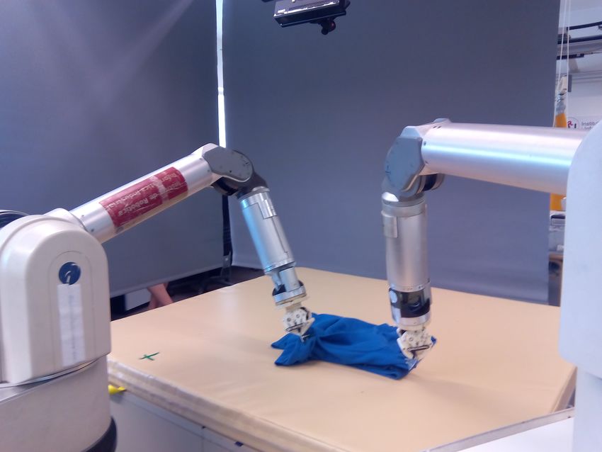
(see Fig. 5(a)). Therefore, the reward function used was: projection on the table (see Fig. 5(a)), expressed as:
#pix. rectangle
(a − aref )2 + (b − bref )2 ,
Rcolor =
R = −Racceleration − Rcolor − Rdepth , (29) #blue pix. rectangle
(30)
where a, b are the measured side lengths of the bounding
rectangle in Fig. 5(a), and aref , bref are their reference val-
where Racceleration is a term penalizing large acceleration ues, given the polo dimensions. Rdepth penalizes the outcome
commands at the joint level, Rcolor has a large penalizing if the polo shirt presents a too wrinkled configuration after
value if the result after the motion does not have a rectangular the motion (see Fig. 5(b)) and it is computed using the codeYou can also read