ESPNet: Efficient Spatial Pyramid of Dilated Convolutions for Semantic Segmentation
←
→
Page content transcription
If your browser does not render page correctly, please read the page content below
ESPNet: Efficient Spatial Pyramid of Dilated
arXiv:1803.06815v3 [cs.CV] 25 Jul 2018
                                             Convolutions for Semantic Segmentation

                                                    Sachin Mehta1 , Mohammad Rastegari2 , Anat Caspi1 ,
                                                         Linda Shapiro1 , and Hannaneh Hajishirzi1
                                                          1
                                                          University of Washington, Seattle, WA, USA
                                             {sacmehta, caspian, shapiro, hannaneh}@cs.washington.edu
                                                   2 Allen Institute for AI and XNOR.AI, Seattle, WA, USA

                                                                   mohammadr@allenai.org
                                                Source code: https://github.com/sacmehta/ESPNet

                                          Abstract. We introduce a fast and efficient convolutional neural network, ES-
                                          PNet, for semantic segmentation of high resolution images under resource con-
                                          straints. ESPNet is based on a new convolutional module, efficient spatial pyra-
                                          mid (ESP), which is efficient in terms of computation, memory, and power. ES-
                                          PNet is 22 times faster (on a standard GPU) and 180 times smaller than the
                                          state-of-the-art semantic segmentation network PSPNet [1], while its category-
                                          wise accuracy is only 8% less. We evaluated ESPNet on a variety of semantic
                                          segmentation datasets including Cityscapes, PASCAL VOC, and a breast biopsy
                                          whole slide image dataset. Under the same constraints on memory and compu-
                                          tation, ESPNet outperforms all the current efficient CNN networks such as Mo-
                                          bileNet [16], ShuffleNet [17], and ENet [20] on both standard metrics and our
                                          newly introduced performance metrics that measure efficiency on edge devices.
                                          Our network can process high resolution images at a rate of 112 and 9 frames per
                                          second on a standard GPU and edge device, respectively.

                                 1       Introduction
                                 Deep convolutional neural network (CNN) models have achieved high accuracy in vi-
                                 sual scene understanding tasks [1–3]. While the accuracy of these networks has im-
                                 proved with their increase in depth and width, large networks are slow and power
                                 hungry. This is especially problematic on the computationally heavy task of seman-
                                 tic segmentation [4–10]. For example, PSPNet [1] has 65.7 million parameters and
                                 runs at about 1 FPS while discharging the battery of a standard laptop at a rate of 77
                                 Watts. Many advanced real-world applications, such as self-driving cars, robots, and
                                 augmented reality, are sensitive and demand on-line processing of data locally on edge
                                 devices. These accurate networks require enormous resources and are not suitable for
                                 edge devices, which have limited energy overhead, restrictive memory constraints, and
                                 reduced computational capabilities.
                                     Convolution factorization has demonstrated its success in reducing the computa-
                                 tional complexity of deep CNNs (e.g. Inception [11–13], ResNext [14], and Xcep-
                                 tion [15]). We introduce an efficient convolutional module, ESP (efficient spatial pyra-
                                 mid), which is based on the convolutional factorization principle (Fig. 1). Based on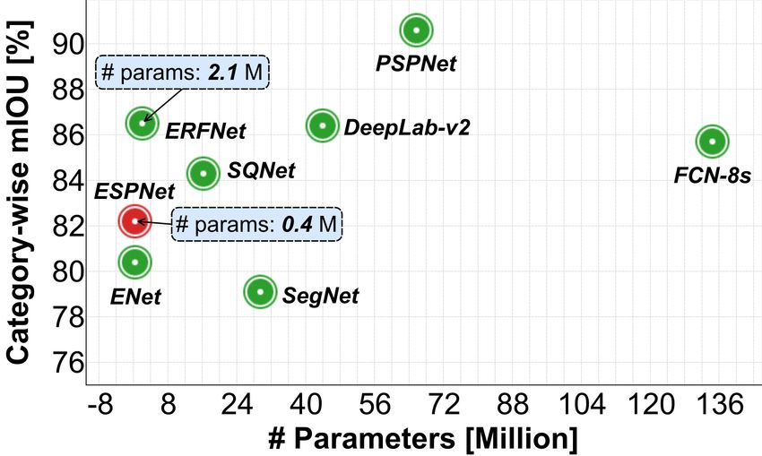
2        Mehta et al.

                                                  ESP Strategy
                                                     Reduce                                                   M, 1 × 1, d

                                                      Split

                                                    Transform       d, n1 × n1, d   d, n2 × n2, d   d, n3 × n3, d · · · d, nK × nK , d

                                                              HFF
                                                                                        Sum
                                                                                                       Sum
                                                                                                                            Sum
                                                     Merge                                                      Concat

                                                                                                                  Sum

                        (a)                                                            (b)

Fig. 1: (a) The standard convolution layer is decomposed into point-wise convolution and spatial
pyramid of dilated convolutions to build an efficient spatial pyramid (ESP) module. (b) Block
diagram of ESP module. The large effective receptive field of the ESP module introduces gridding
artifacts, which are removed using hierarchical feature fusion (HFF). A skip-connection between
input and output is added to improve the information flow. See Section 3 for more details. Dilated
convolutional layers are denoted as (# input channels, effective kernel size, # output channels).
The effective spatial dimensions of a dilated convolutional kernel are nk × nk , where nk = (n −
1)2k−1 + 1, k = 1, · · · , K. Note that only n × n pixels participate in the dilated convolutional
kernel. In our experiments n = 3 and d = M  K.

these ESP modules, we introduce an efficient network structure, ESPNet, that can be
easily deployed on resource-constrained edge devices. ESPNet is fast, small, low power,
and low latency, yet still preserves segmentation accuracy.
    ESP is based on a convolution factorization principle that decomposes a standard
convolution into two steps: (1) point-wise convolutions and (2) spatial pyramid of di-
lated convolutions, as shown in Fig. 1. The point-wise convolutions help in reducing
the computation, while the spatial pyramid of dilated convolutions re-samples the fea-
ture maps to learn the representations from large effective receptive field. We show that
our ESP module is more efficient than other factorized forms of convolutions, such as
Inception [11–13] and ResNext [14]. Under the same constraints on memory and com-
putation, ESPNet outperforms MobileNet [16] and ShuffleNet [17] (two other efficient
networks that are built upon the factorization principle). We note that existing spatial
pyramid methods (e.g. the atrous spatial pyramid module in [3]) are computationally
expensive and cannot be used at different spatial levels for learning the representa-
tions. In contrast to these methods, ESP is computationally efficient and can be used at
different spatial levels of a CNN network. Existing models based on dilated convolu-
tions [1, 3, 18, 19] are large and inefficient, but our ESP module generalizes the use of
dilated convolutions in a novel and efficient way.
    To analyze the performance of a CNN network on edge devices, we introduce sev-
eral new performance metrics, such as sensitivity to GPU frequency and warp execution
efficiency. To showcase the power of ESPNet, we evaluate our model on one of the most
expensive tasks in AI and computer vision: semantic segmentation. ESPNet is empir-
ically demonstrated to be more accurate, efficient, and fast than ENet [20], one of the
most power-efficient semantic segmentation networks, while learning a similar number
of parameters. Our results also show that ESPNet learns generalizable representations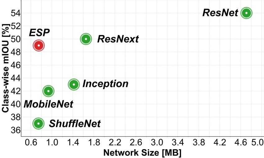
ESPNet: Efficient Spatial Pyramid of Dilated Convolutions for Semantic Segmentation         3

and outperforms ENet [20] and another efficient network ERFNet [21] on the unseen
dataset. ESPNet can process a high resolution RGB image at a rate of 112 frames per
second (FPS) on a high-end GPU, 21 FPS on a laptop, and 9 FPS on an edge device3 .

2     Related Work

Multiple different techniques, such as convolution factorization, network compression,
and low-bit networks, have been proposed to speed up convolutional neural networks.
We, first, briefly describe these approaches and then provide a brief overview of CNN-
based semantic segmentation.
Convolution factorization: Convolutional factorization decomposes the convolutional
operation into multiple steps to reduce the computational complexity. This factoriza-
tion has successfully shown its potential in reducing the computational complexity of
deep CNN networks (e.g. Inception [11–13], factorized network [22], ResNext [14],
Xception [15], and MobileNets [16]). ESP modules are also built on this factorization
principle. The ESP module decomposes a convolutional layer into a point-wise convo-
lution and spatial pyramid of dilated convolutions. This factorization helps in reducing
the computational complexity, while simultaneously allowing the network to learn the
representations from a large effective receptive field.
Network Compression: Another approach for building efficient networks is compres-
sion. These methods use techniques such as hashing [23], pruning [24], vector quanti-
zation [25], and shrinking [26, 27] to reduce the size of the pre-trained network.
Low-bit networks: Another approach towards efficient networks is low-bit networks,
which quantize the weights to reduce the network size and complexity (e.g. [28–31]).
Sparse CNN: To remove the redundancy in CNNs, sparse CNN methods, such as sparse
decomposition [32], structural sparsity learning [33], and dictionary-based method [34],
have been proposed.
    We note that compression-based methods, low-bit networks, and sparse CNN meth-
ods are equally applicable to ESPNets and are complementary to our work.
Dilated convolution: Dilated convolutions [35] are a special form of standard convo-
lutions in which the effective receptive field of kernels is increased by inserting zeros
(or holes) between each pixel in the convolutional kernel. For a n × n dilated convolu-
tional kernel with a dilation rate of r, the effective size of the kernel is [(n − 1)r + 1]2 .
The dilation rate specifies the number of zeros (or holes) between pixels. However, due
to dilation, only n × n pixels participate in the convolutional operation, reducing the
computational cost while increasing the effective kernel size.
    Yu and Koltun [18] stacked dilated convolution layers with increasing dilation rate
to learn contextual representations from a large effective receptive field. A similar strat-
egy was adopted in [19, 36, 37]. Chen et al. [3] introduced an atrous spatial pyramid
(ASP) module. This module can be viewed as a parallelized version of [3]. These mod-
ules are computationally inefficient (e.g. ASPs have high memory requirements and
learn many more parameters; see Section 3.2). Our ESP module also learns multi-scale
 3   We used a desktop with NVIDIA TitanX GPU, a laptop with GTX-960M GPU, and NVIDIA
     Jetson TX2 as an edge device. See Appendix A for more details.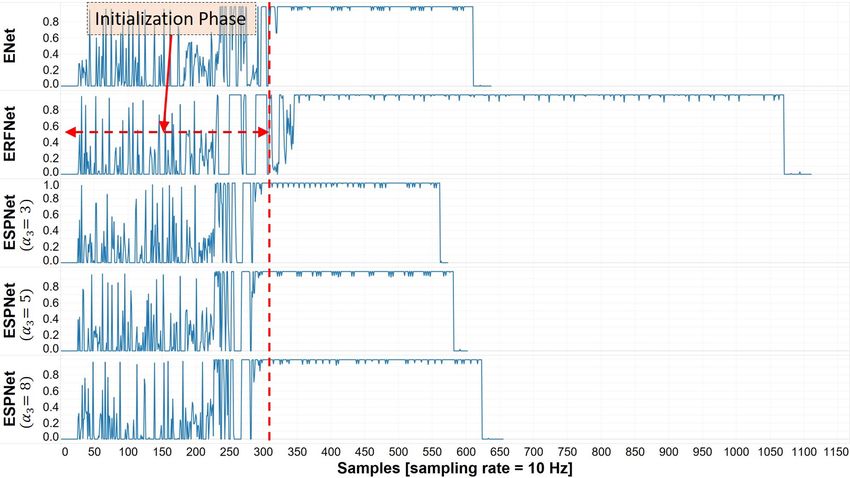
4       Mehta et al.

representations using dilated convolutions in parallel; however, it is computationally
efficient and can be used at any spatial level of a CNN network.
CNN for semantic segmentation: Different CNN-based segmentation networks have
been proposed, such as multi-dimensional recurrent neural networks [38], encoder-
decoders [20, 21, 39, 40], hypercolumns [41], region-based representations [42, 43], and
cascaded networks [44]. Several supporting techniques along with these networks have
been used for achieving high accuracy, including ensembling features [3], multi-stage
training [45], additional training data from other datasets [1, 3], object proposals [46],
CRF-based post processing [3], and pyramid-based feature re-sampling [1–3].
Encoder-decoder networks: Our work is related to this line of work. The encoder-
decoder networks first learn the representations by performing convolutional and down-
sampling operations. These representations are then decoded by performing up-sampling
and convolutional operations. ESPNet first learns the encoder and then attaches a light-
weight decoder to produce the segmentation mask. This is in contrast to existing net-
works where the decoder is either an exact replica of the encoder (e.g. [39]) or is rela-
tively small (but not light weight) in comparison to the encoder (e.g. [20, 21]).
Feature re-sampling methods: The feature re-sampling methods re-sample the convo-
lutional feature maps at the same scale using different pooling rates [1, 2] and kernel
sizes [3] for efficient classification. Feature re-sampling is computationally expensive
and is performed just before the classification layer to learn scale-invariant representa-
tions. We introduce a computationally efficient convolutional module that allows feature
re-sampling at different spatial levels of a CNN network.

3     ESPNet
This section elaborates on the details of ESPNET and describes the core ESP module
on which it is built. We compare ESP modules with similar CNN modules, such as
Inception [11–13], ResNext [14], MobileNet [16], and ShuffleNet [17] modules.

3.1   ESP module
ESPNet is based on efficient spatial pyramid (ESP) modules, which are a factorized
form of convolutions that decompose a standard convolution into a point-wise convolu-
tion and a spatial pyramid of dilated convolutions (see Fig. 1a). The point-wise convolu-
tion in the ESP module applies a 1 × 1 convolution to project high-dimensional feature
maps onto a low-dimensional space. The spatial pyramid of dilated convolutions then
re-samples these low-dimensional feature maps using K, n × n dilated convolutional
kernels simultaneously, each with a dilation rate of 2k−1 , k = {1, · · · , K}. This factor-
ization drastically reduces the number of parameters and the memory required by the
                                                                                    2
ESP module, while preserving a large effective receptive field (n − 1)2K−1 + 1 . This


pyramidal convolutional operation is called a spatial pyramid of dilated convolutions,
because each dilated convolutional kernel learns weights with different receptive fields
and so resembles a spatial pyramid.
    A standard convolutional layer takes an input feature map Fi ∈ RW ×H×M and ap-
plies N kernels K ∈ Rm×n×M to produce an output feature map Fo ∈ RW ×H×N , where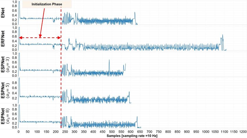
ESPNet: Efficient Spatial Pyramid of Dilated Convolutions for Semantic Segmentation                   5

W and H represent the width and height of the feature map, m and n represent the
width and height of the kernel, and M and N represent the number of input and output
feature channels. For the sake of simplicity, we will assume that m = n. A standard con-
volutional kernel thus learns n2 MN parameters. These parameters are multiplicatively
dependent on the spatial dimensions of the n × n kernel and the number of input M and
output N channels.
Width divider K: To reduce the computational cost, we introduce a simple hyper-
parameter K. The role of K is to shrink the dimensionality of the feature maps uniformly
across each ESP module in the network. Reduce: For a given K, the ESP module first
reduces the feature maps from M-dimensional space to NK -dimensional space using a
point-wise convolution (Step 1 in Fig. 1a). Split: The low-dimensional feature maps
are then split across K parallel branches. Transform: Each branch then processes these
feature maps simultaneously using n × n dilated convolutional kernels with different
dilation rates given by 2k−1 , k = {1, · · · , K − 1} (Step 2 in Fig. 1a). Merge: The output
of these K parallel dilated convolutional kernels is then concatenated to produce an N-
dimensional output feature map4 . Fig. 1b visualizes the reduce-split-transform-merge
strategy used in ESP modules.
                                      (nN)    2
    The ESP module has MN       K + K       parameters and its effective receptive field is
                    2
           K−1 + 1 . Compared to the n2 NM parameters of the standard convolution,

 (n − 1)2
factorizing it using the two steps reduces the total number of parameters in the ESP
                        n2 MK                                                            K−1 ]2 .
module by a factor of M+n   2 N , while increasing the effective receptive field by ∼ [2
For example, an ESP module learns ∼ 3.6 times fewer parameters with an effective re-
ceptive field of 17 × 17 than a standard convolutional kernel with an effective receptive
field of 3 × 3 for n = 3, N = M = 128, and K = 4.
Hierarchical feature fusion (HFF) for de-gridding: While concatenating the outputs
of dilated convolutions give the ESP module a large effective receptive field, it intro-
duces unwanted checkerboard or gridding artifacts, as shown in Fig. 2. To address the
gridding artifact in ESP, the feature maps obtained using kernels of different dilation
rates are hierarchically added before concatenating them (HFF in Fig. 1b). This solu-
tion is simple and effective and does not increase the complexity of the ESP module, in
contrast to existing methods that remove the gridding artifact by learning more parame-
ters using dilated convolutional kernels with small dilation rates [19,37]. To improve the
gradient flow inside the network, the input and output feature maps of the ESP module
are combined using an element-wise sum [47].

3.2     Relationship with other CNN modules

The ESP module shares similarities with the following CNN modules.
MobileNet module: The MobileNet module [16], visualized in Fig. 3a, uses a depth-
wise separable convolution [15] that factorizes a standard convolutions into depth-wise
 4   In general, N                                                                       N
                  K may not be a perfect divisor, and therefore concatenating K, K -dimensional
     feature maps would         not result in an N-dimensional output. To handle this, we use
      N − (K − 1)b N                 with a dilation rate of 20 and b N

                    K c      kernels                                  K c kernels for each dilation rate
     2 k−1 for k = {2, · · · , K}.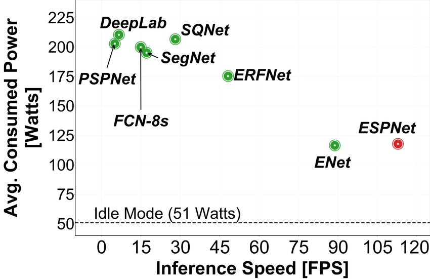
6        Mehta et al.

                                 RGB                  without HFF                with HFF

         (a)                                               (b)

Fig. 2: (a) An example illustrating a gridding artifact with a single active pixel (red) convolved
with a 3 ×3 dilated convolutional kernel with dilation rate r = 2. (b) Visualization of feature maps
of ESP modules with and without hierarchical feature fusion (HFF). HFF in ESP eliminates the
gridding artifact. Best viewed in color.

convolutions (transform) and point-wise convolutions (expand). It learns less parame-
ters, has high memory requirement, and low receptive field than the ESP module. An
extreme version of the ESP module (with K = N) is almost identical to the MobileNet
module, differing only in the order of convolutional operations. In the MobileNet mod-
ule, the spatial convolutions are followed by point-wise convolutions; however, in the
ESP module, point-wise convolutions are followed by spatial convolutions. Note that
                                                                    2
the effective receptive field of an ESP module ( (n − 1)2K−1 + 1 ) is higher than a


MobileNet module ([n]2 ).
ShuffleNet module: The ShuffleNet module [17], shown in Fig. 3b, is based on the
principle of reduce-transform-expand. It is an optimized version of the bottleneck block
in ResNet [47]. To reduce computation, Shufflenet makes use of grouped convolu-
tions [48] and depth-wise convolutions [15]. It replaces 1 × 1 and 3 × 3 convolutions in
the bottleneck block in ResNet with 1 × 1 grouped convolutions and 3 × 3 depth-wise
separable convolutions, respectively. The Shufflenet module learns many less parame-
ters than the ESP module, but has higher memory requirements and a smaller receptive
field.
Inception module: Inception modules [11–13] are built on the principle of split-reduce-
transform-merge. These modules are usually heterogeneous in number of channels and
kernel size (e.g. some of the modules are composed of standard and factored convo-
lutions). In contrast to the Inception modules, ESP modules are straightforward and
simple to design. For the sake of comparison, the homogeneous version of an Inception
module is shown in Fig. 3c. Fig. 3g compares the Inception module with the ESP mod-
ule. ESP (1) learns fewer parameters, (2) has a low memory requirement, and (3) has a
larger effective receptive field.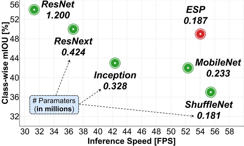
ESPNet: Efficient Spatial Pyramid of Dilated Convolutions for Semantic Segmentation                                                                                                7

ResNext module: A ResNext module [14], shown in Fig. 3d, is a parallel version of
the bottleneck module in ResNet [47] and is based on the principle of split-reduce-
transform-expand-merge. The ESP module is similar to ResNext in the sense that it
involves branching and residual summation. However, the ESP module is more efficient
in memory and parameters and has a larger effective receptive field.
Atrous spatial pyramid (ASP) module: An ASP module [3], shown in Fig. 3e, is built
on the principle of split-transform-merge. The ASP module involves branching with
each branch learning kernel at a different receptive field (using dilated convolutions).
Though ASP modules tend to perform well in segmentation tasks due to their high
effective receptive fields, ASP modules have high memory requirements and learn many
more parameters. Unlike the ASP module, the ESP module is computationally efficient.

    Convolution Type
           Depth-wise
           Grouped                                       M, 1 × 1, d
                  Standard
                                                          d, 3 × 3, d                              M, 1 × 1, d           M, 1 × 1, d · · · M, 1 × 1, d
         M, 3 × 3, M
                                                         d, 1 × 1, N                               d, n × n, d           d, n × n, d · · · d, n × n, d
          M, 1 × 1, N
                                                               Sum                                                                               Concat
          MobileNet

   (a) MobileNet                                    (b) ShuffleNet                                             (c) Inception
                                                                                                                                                            M, 1 × 1, d

    M, 1 × 1, d    M, 1 × 1, d · · · M, 1 × 1, d
    d, n × n, d    d, n × n, d · · · d, n × n, d                                                                 d, n1 × n1, d   d, n2 × n2, d    d, n3 × n3, d · · · d, nK × nK , d

    d, 1 × 1, N    d, 1 × 1, N · · · d, 1 × 1, N         20             21                      2K−1
                                                                                                         HFF

                                                                                                                                     Sum
                                                        M, n × n, N    M, n × n, N · · · M, n × n, N                                                 Sum
                                                                                                                                                                          Sum
                               Sum                                                                                                                            Concat

                               Sum                                                Sum                                                                           Sum

            (d) ResNext                                               (e) ASP                           (f) ESP (same as in Fig. 1)
Module                                             # Parameters             Memory (in MB)                     Effective Receptive Field
MobileNet                             M(n2 + N) = 11, 009               (M + N)W H = 2.39                                                          [n]2 = 3 × 3
ShuffleNet                      d             2
                                g (M + N) + n d = 2,180               W H(2 ∗ d + N) = 1.67                                                        [n]2 = 3 × 3
Inception                                 2 2
                                K(Md + n d ) = 28, 000                    2KW Hd = 2.39                    [n]2 = 3 × 3
ResNext               K(Md + d 2 n2 + dN) = 38, 000                   KW H(2d + N) = 8.37                  [n]2 = 3 × 3
                                                                                                          2
                                         KMNn2 = 450, 000                                          K−1

ASP                                                                         KW HN = 5.98 (n − 1)2      + 1 = 33 × 33
                                                                                                          2
                                   Md + Kn2 d 2 = 20, 000               W Hd(K + 1) = 1.43 (n − 1)2K−1 + 1 = 33 × 33

ESP (Fig. 1b)
                                                           N
Here, M = N = 100, n = 3, K = 5, d =                       K   = 20, g = 2, and W = H = 56.
                                           (g) Comparison between different modules

Fig. 3: Different types of convolutional modules for comparison. We denote the layer as (# input
channels, kernel size, # output channels). Dilation rate in (e) is indicated on top of each layer.
Here, g represents the number of convolutional groups in grouped convolution [48]. For simplic-
ity, we only report the memory of convolutional layers in (d). For converting the required memory
to bytes, we multiply it by 4 (1 float requires 4 bytes for storage).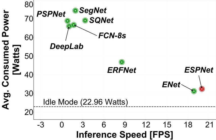
8         Mehta et al.

4     Experiments

Semantic segmentation is one of the most expensive task in AI and computer vision. To
showcase the power of ESPNet, ESPNet’s performance is evaluated on several datasets
for semantic segmentation and compared to the state-of-the-art networks.

4.1    Experimental set-up

Network structure: ESPNet uses ESP modules for learning convolutional kernels as
well as down-sampling operations, except for the first layer which is a standard strided
convolution. All layers (convolution and ESP modules) are followed by a batch normal-
ization [49] and a PReLU [50] non-linearity except for the last point-wise convolution,
which has neither batch normalization nor non-linearity. The last layer feeds into a soft-
max for pixel-wise classification.
    Different variants of ESPNet are shown in Fig. 4. The first variant, ESPNet-A (Fig.
4a), is a standard network that takes an RGB image as an input and learns represen-
tations at different spatial levels5 using the ESP module to produce a segmentation
mask. The second variant, ESPNet-B (Fig. 4b), improves the flow of information inside
ESPNet-A by sharing the feature maps between the previous strided ESP module and
the previous ESP module. The third variant, ESPNet-C (Fig. 4c), reinforces the input
image inside ESPNet-B to further improve the flow of information. These three vari-
ants produce outputs whose spatial dimensions are 18 th of the input image. The fourth
variant, ESPNet (Fig. 4d), adds a light weight decoder (built using a principle of reduce-
upsample-merge) to ESPNet-C that outputs the segmentation mask of the same spatial
resolution as the input image.
    To build deeper computationally efficient networks for edge devices without chang-
ing the network topology, a hyper-parameter α controls the depth of the network; the
ESP module is repeated αl times at spatial level l. CNNs require more memory at higher
spatial levels (at l = 0 and l = 1) because of the high spatial dimensions of feature maps
at these levels. To be memory efficient, neither the ESP nor the convolutional mod-
ules are repeated at these spatial levels. The building block functions used to build the
ESPNet (from ESPNet-A to ESPNet) are discussed in Appendix B.
Dataset: We evaluated the ESPNet on the Cityscapes dataset [6], an urban visual scene
understanding dataset that consists of 2,975 training, 500 validation, and 1,525 test
high-resolution images. The dataset was captured across 50 cities and in different sea-
sons. The task is to segment an image into 19 classes belonging to 7 categories (e.g.
person and rider classes belong to the same category human). We evaluated our net-
works on the test set using the Cityscapes online server.
    To study the generalizability, we tested the ESPNet on an unseen dataset. We used
the Mapillary dataset [51] for this task because of its diversity. We mapped the anno-
tations (65 classes) in the validation set (# 2,000 images) to seven categories in the
Cityscape dataset. To further study the segmentation power of our model, we trained
and tested the ESPNet on two other popular datasets from different domains. First,
5   At each spatial level l, the spatial dimensions of the feature maps are the same. To learn repre-
    sentations at different spatial levels, a down-sampling operation is performed (see Fig. 4a).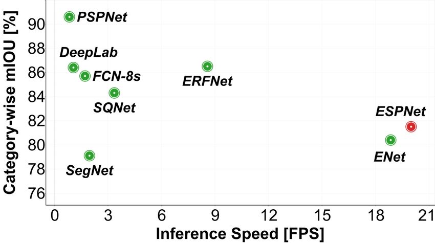
ESPNet: Efficient Spatial Pyramid of Dilated Convolutions for Semantic Segmentation                                          9

         RGB Image                 RGB Image                RGB Image             RGB Image            Segmentation Mask

l=0
                                            (3, 16)                  (3, 16)
                                                                                                                   (C, C)
                                                              Conv-3
                 (3, 16)             Conv-3                                                                DeConv
 l=1     Conv-3                           (16, 64)
                                                              Concat
                                                                                          (3, 16)                  (2C, C)
                 (16, 64)             ESP                                          Conv-3                   Conv-1
                                                                     (19, 64)
 l=2       ESP                              (64, 64)           ESP                              (19, C)
                                      ESP
                   (64, 64)                                          (64, 64)      Concat       Conv-1      Concat
                                      ×α2                      ESP
           ESP                                                                            (19, 64)                 (C, C)
                                                               ×α2
 l=2                                                                                ESP
           ×α2                       Concat                                                                DeConv
                                          (128, 128)          Concat                      (64, 64)
                 (64, 128)                                                          ESP                            (2C, C)
                                      ESP                            (131, 128)
 l=3       ESP                              (128, 128)         ESP
                                                                                    ×α2                      ESP
                                                                                               (131, C)
                   (128, 128)         ESP                            (128, 128)
                                      ×α3                      ESP                 Concat       Conv-1      Concat
           ESP                                                 ×α3
 l=3                                                                                      (131, 128)
           ×α3
                                     Concat                                         ESP                            (C, C)
                 (128, C)                                     Concat
                                          (256, C)                                        (128, 128)       DeConv
                                                                     (256, C)
 l=3     Conv-1                      Conv-1                   Conv-1
                                                                                    ESP
                                                                                    ×α3
                                                                                               (256, C)
      Segmentation Mask         Segmentation Mask        Segmentation Mask         Concat       Conv-1

 (a) ESPNet-A                     (b) ESPNet-B            (c) ESPNet-C                      (d) ESPNet

Fig. 4: The path from ESPNet-A to ESPNet. Red and green color boxes represent the modules
responsible for down-sampling and up-sampling operations, respectively. Spatial-level l is indi-
cated on the left of every module in (a). We denote each module as (# input channels, # output
channels). Here, Conv-n represents n × n convolution.

we used the widely known PASCAL VOC dataset [52] that has 1,464 training images,
1,448 validation images, and 1,456 test images. The task is to segment an image into
20 foreground classes. We evaluate our networks on the test set (comp6 category) using
the PASCAL VOC online server. Following the convention, we used additional images
from [53,54]. Secondly, we used a breast biopsy whole slide image dataset [36], chosen
because tissue structures in biomedical images vary in size and shape and because this
dataset allowed us to check the potential of learning representations from a large recep-
tive field. The dataset consists of 30 training images and 28 validation images, whose
average size is 10, 000 × 12, 000, much larger than natural scene images. The task is to
segment the images into 8 biological tissue labels; details are in [36].
Performance evaluation metrics: Most traditional CNNs measure network perfor-
mance in terms of accuracy, latency, number of network parameters, and network size
(e.g. [16, 17, 20, 21, 55]). These metrics provide high-level insight about the network,
but fail to demonstrate the efficient usage of limited available hardware resources. In
addition to these metrics, we introduce several system-level metrics to characterize the
performance of a CNN on resource-constrained devices [56, 57].
Segmentation accuracy is measured as a mean Intersection over Union (mIOU) score
between the ground truth and the predicted segmentation mask.
Latency represents the amount of time a CNN network takes to process an image. This
is usually measured in terms of frames per second (FPS).
Network parameters represents the number of parameters learned by the network.
10      Mehta et al.

Network size represents the amount of storage space required to store the network pa-
rameters. An efficient network should have a smaller network size.
Sensitivity to GPU frequency measures the computational capability of an application
and is defined as a ratio of percentage change in execution time to the percentage change
in GPU frequency. A higher value indicates that the application tends to utilize the GPU
more efficiently.
Utilization rates measures the utilization of compute resources (CPU, GPU, and mem-
ory) while running on an edge device. In particular, computing units in edge devices
(e.g. Jetson TX2) share memory between CPU and GPU.
Warp execution efficiency is defined as the average percentage of active threads in each
executed warp. GPUs schedule threads in the form of warps, and each thread inside
the warp is executed in single instruction multiple data fashion. A high value of warp
execution efficiency represents efficient usage of GPU.
Memory efficiency is the ratio of number of bytes requested/stored to the number of
bytes transfered from/to device (or shared) memory to satisfy load/store requests. Since
memory transactions are in blocks, this metric allows us to determine how efficiently
we are using the memory bandwidth.
Power consumption is the amount of average power consumed by the application dur-
ing inference.
Training details: ESPNet networks were trained using PyTorch [58] with CUDA 9.0
and cuDNN back-ends. ADAM [59] was used with an initial learning rate of 0.0005,
and decayed by two after every 100 epochs and with a weight decay of 0.0005. An
inverse class probability weighting scheme was used in the cross-entropy loss function
to address the class imbalance [20, 21]. Following [20, 21], the weights were initial-
ized randomly. Standard strategies, such as scaling, cropping and flipping, were used
to augment the data. The image resolution in the Cityscape dataset is 2048 × 1024, and
all the accuracy results were reported at this resolution. For training the networks, we
sub-sampled the RGB images by two. When the output resolution was smaller than
2048 × 1024, the output was up-sampled using bi-linear interpolation. For training on
the PASCAL dataset, we used a fixed image size of 512 × 512. For the WSI dataset,
the patch-wise training approach was followed [36]. ESPNet was trained in two stages.
First, ESPNet-C was trained with down-sampled annotations. Second, a light-weight
decoder was attached to ESPNet-C and then, the entire ESPNet network was trained.
    Three different GPU devices were used for our experiments: (1) a desktop with a
NVIDIA TitanX GPU (3,584 CUDA cores), (2) a laptop with a NVIDIA GTX-960M
GPU (640 CUDA cores), and (3) an edge device with NVIDIA Jetson TX2 (256 CUDA
cores). See Appendix A for more details about the hardware. Unless and otherwise
stated explicitly, statistics, such as power consumption and inference speed, are re-
ported for an RGB image of size 1024 × 512 averaged over 200 trials. For collecting
the hardware-level statistics, NVIDIA’s and Intel’s hardware profiling and tracing tools,
such as NVPROF [60], Tegrastats [61], and PowerTop [62], were used. In our experi-
ments, we will refer to ESPNet with α2 = 2 and α3 = 8 as ESPNet until and otherwise
stated explicitly.
ESPNet: Efficient Spatial Pyramid of Dilated Convolutions for Semantic Segmentation 11
4.2 Results on the Cityscape dataset
Comparison with state-of-the-art efficient convolutional modules: In order to under-
stand the ESP module, we replaced the ESP modules in ESPNet-C with state-of-the-art
efficient convolutional modules, sketched in Fig. 3 (MobileNet [16], ShuffleNet [17],
Inception [11–13], ResNext [14], and ResNet [47]) and evaluate their performance on
the Cityscape validation dataset. We did not compare with ASP [3], because it is compu-
tationally expensive and not suitable for edge devices. Fig. 5 compares the performance
of ESPNet-C with different convolutional modules. Our ESP module outperformed Mo-
bileNet and ShuffleNet modules by 7% and 12%, respectively, while learning a similar
number of parameters and having comparable network size and inference speed. Fur-
thermore, the ESP module delivered comparable accuracy to ResNext and Inception
more efficiently. A basic ResNet module (stack of two 3 × 3 convolutions with a skip-
connection) delivered the best performance, but had to learn 6.5× more parameters.
Comparison with state-of-the-art segmentation methods: We compared the perfor-
mance of ESPNet with state-of-the-art semantic segmentation networks. These net-
works either use a pre-trained network (VGG [63]: FCN-8s [45] and SegNet [39],
ResNet [47]: DeepLab-v2 [3] and PSPNet [1], and SqueezeNet [55]: SQNet [64]) or
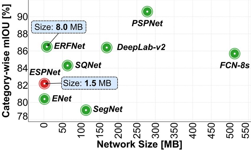
were trained from scratch (ENet [20] and ERFNet [21]). Fig. 6 compares ESPNet with
state-of-the-art methods. ESPNet is 2% more accurate than ENet [20], while running
1.27× and 1.16× faster on a desktop and a laptop, respectively. ESPNet makes some
mistakes between classes that belong to the same category, and hence has a lower class-
wise accuracy (see Appendix F for the confusion matrix). For example, a rider can be
confused with a person. However, ESPNet delivers a good category-wise accuracy. ES-
PNet had 8% lower category-wise mIOU than PSPNet [1], while learning 180× fewer
parameters. ESPNet had lower power consumption, had lower battery discharge rate,
and was significantly faster than state-of-the-art methods, while still achieving a com-
petitive category-wise accuracy; this makes ESPNet suitable for segmentation on edge
devices. ERFNet, an another efficient segmentation network, delivered good segmenta-
tion accuracy, but has 5.5× more parameters, is 5.44× larger, consumes more power,
(a) Accuracy vs. network size (b) Accuracy vs. speed (laptop)
Fig. 5: Comparison between state-of-the-art efficient convolutional modules. For a fair compari-
son between different modules, we used K = 5, d = N K , α2 = 2, and α3 = 3. We used standard
strided convolution for down-sampling. For ShuffleNet, we used g = 4 and K = 4 so that the
resultant ESPNet-C network has the same complexity as with the ESP block.12 Mehta et al.
mIOU
Network Class Category
ENet [20] 58.3 80.4
ERFNet [21] 68.0 86.5
SQNet [27] 59.8 84.3
SegNet [39] 57.0 79.1
ESPNet (Ours) 60.3 82.2
FCN-8s [39] 65.3 85.7
DeepLab-v2 [3] 70.4 86.4
PSPNet [1] 78.4 90.6
(a) Test set (b) Accuracy vs. network size (c) Accuracy vs. # parameters
(d) Battery discharge rate vs. network (laptop) (e) Accuracy vs. speed (laptop)
(f) Power consumption vs. speed (laptop) (g) Power consumption vs. speed (desktop)
Fig. 6: Comparison between state-of-the-art segmentation methods on the Cityscape test set on
two different devices. All networks (FCN-8s [45], SegNet [39], SQNet [64], ENet [20], DeepLab-
v2 [3], PSPNet [1], and ERFNet [21]) were without conditional random field and converted to
PyTorch for a fair comparison. Best viewed in color.
and has a higher battery discharge rate than ESPNet. Also, ERFNet does not utilize
limited available hardware resources efficiently on edge devices (Section 4.4).
4.3 Segmentation results on other datasets
Unseen dataset: Table 1a compares the performance of ESPNet to that of ENet [20]
and ERFNet [21] on an unseen dataset. These networks were trained on the Cityscapes
dataset [6] and tested on the Mapillary (unseen) dataset [51]. ENet and ERFNet were
chosen, because ENet was one of the most power efficient segmentation networks, while
ERFNet has high accuracy and moderate efficiency. Our experiments show that ESPNet
learns good generalizable representations of objects and outperforms ENet and ERFNet
both qualitatively and quantitatively on the unseen dataset.ESPNet: Efficient Spatial Pyramid of Dilated Convolutions for Semantic Segmentation 13
mIOU # Params
ENet [20] 0.33 0.364
ERFNet [21] 0.25 2.06
ESPNet 0.40 0.364
(a) Mapillary validation set [51] (b) Mapillary validation set [51] (unseen)
Model ESPNet SegNet RefineNet DeepLab PSPNet LRR Dilation-8 FCN-8s Model Module mIOU # Params
(Ours) [39] [44] [3] [1] [65] [18] [45]
ESPNet (Ours)? ESP 44.03 2.75
# Params 0.364 29.5 42.6 44.04 65.7 48 141.13 134.5 SegNet [39] VGG 37.6 12.80
mIOU 63.01 59.10 82.40 79.70 85.40 79.30 75.30 67.20 Mehta et al. [36] ResNet 44.20 26.03
(c) PASCAL VOC test set [52] (d) Breast biopsy validation set [36]
Table 1: Results on different datasets. Here, the number of parameters are in million. ? For more
details, please see [66]. See Appendix F for more qualitative results.
PASCAL VOC 2012 dataset: (Table 1c) On the PASCAL dataset, ESPNet is 4% more
accurate than SegNet, one of the smallest network on the PASCAL VOC, while learning
81× fewer parameters. ESPNet is 22% less accurate than PSPNet (one of the most
accurate network on the PASCAL VOC) while learning 180× fewer parameters.
Breast biopsy dataset: (Table 1d) On the breast biopsy dataset, ESPNet achieved the
same accuracy as [36] while learning 9.5× less parameters.
4.4 Performance analysis on an edge device
We measure the performance on the NVIDIA Jetson TX2, a computing platform for
edge devices. Performance analysis results are given in Fig. 7.
Network size: Fig. 7a compares the uncompressed 32-bit network size of ESPNet with
ENet and ERFNet. ESPNet had a 1.12× and 5.45× smaller network than ENet and
ERFNet, respectively, which reflects well on the architectural design of ESPNet.
Inference speed and sensitivity to GPU frequency: Fig. 7b compares the inference
speed of ESPNet with ENet and ERFNet. ESPNet had almost the same frame rate as
ENet, but it was more sensitive to GPU frequency (Fig. 7c). As a consequence, ESPNet
achieved a higher frame rate than ENet on high-end graphic cards, such as the GTX-
960M and TitanX (see Fig. 6). For example, ESPNet is 1.27× faster than ENet on an
NVIDIA TitanX. ESPNet is about 3× faster than ERFNet on an NVIDIA Jetson TX2.
Utilization rates: Fig. 7d compares the CPU, GPU, and memory utilization rates of
different networks. These networks are throughput intensive, and therefore, GPU uti-
lization rates are high, while CPU utilization rates are low for these networks. Memory
utilization rates are significantly different for these networks. The memory footprint of
ESPNet is low in comparison to ENet and ERFNet, suggesting that ESPNet is suitable
for memory-constrained devices.
Warp execution efficiency: Fig. 7e compares the warp execution efficiency of ESPNet
with ENet and ERFNet. The warp execution of ESPNet was about 9% higher than
ENet and about 14% higher than ERFNet. This indicates that ESPNet has less warp14 Mehta et al.
Sensitivity to GPU freq. Utilization (%)
Network Size Network Network
828 to 1134 1134 to 1300 CPU GPU Memory
ENet 1.64 MB ENet 71% 70% ENet 20.5 99.00 50.6
ERFNet 7.95 MB ERFNet 69% 53% ERFNet 19.7 99.00 61.3
ESPNet 1.46 MB ESPNet 86% 95% ESPNet 20.3 99.00 44.0
(a) (b) (c) (d)
(e) (f) GPU freq. @ 828 MHz (g) GPU freq. @ 1,134 MHz
Fig. 7: Performance analysis of ESPNet with ENet and ERFNet on a NVIDIA Jetson TX2: (a)
network size, (b) inference speed vs. GPU frequency (in MHz), (c) sensitivity analysis, (d) uti-
lization rates, (e) efficiency rates, and (f, g) power consumption at two different GPU frequencies.
In (d), the statistics for the network’s initialization phase were not considered, because they were
the same across all networks. See Appendix E for time vs. utilization plots. Best viewed in color.
divergence and promotes the efficient usage of limited GPU resources available on edge
devices. We note that warp execution efficiency gives a better insight into the utilization
of GPU resources than the GPU utilization rate. GPU frequency will be busy even if
few warps are active, resulting in a high GPU utilization rate.
Memory efficiency: (Fig. 7e) All networks have similar global load efficiency, but
ERFNet has a poor store and shared memory efficiency. This is likely due to the fact that
ERFNet spends 20% of the compute power performing memory alignment operations,
while ESPNet and ENet spend 4.2% and 6.6% time for this operation, respectively. See
Appendix D for the compute-wise break down of different kernels.
Power consumption: Fig. 7f and 7g compares the power consumption of ESPNet with
ENet and ERFNet at two different GPU frequencies. The average power consumption
(during network execution phase) of ESPNet, ENet, and ERFNet were 1 W, 1.5 W, and
2.9 W at a GPU frequency of 824 MHz and 2.2 W, 4.6 W, and 6.7 W at a GPU frequency
of 1,134 MHz, respectively; suggesting ESPNet is a power-efficient network.
4.5 Ablation studies on the Cityscapes: The path from ESPNet-A to ESPNet
Larger networks or ensembling the output of multiple networks delivers better perfor-
mance [1, 3, 19], but with ESPNet (sketched in Fig. 4), the goal is an efficient network
for edge devices. To improve the performance of ESPNet while maintaining efficiency,
a systematic study of design choices was performed. Table 2 summarizes the results.
ReLU vs PReLU: (Table 2a) Replacing ReLU [67] with PReLU [50] in ESPNet-A im-
proved the accuracy by 2%, while having a minimal impact on the network complexity.
Residual learning in ESP: (Table 2b) The accuracy of ESPNet-A dropped by about
2% when skip-connections in ESP (Fig. 1b) modules were removed. This verifies the
effectiveness of the residual learning.ESPNet: Efficient Spatial Pyramid of Dilated Convolutions for Semantic Segmentation 15
ESPNet-C ESP operations # params Network
Module mIOU # Params◦ configuration Reduce Transform size mIOU
mIOU # Params◦ Downsample mIOU # Params◦
ESP 0.39 0.183 C1 - (α3 = 3) 3×3 SPC 0.276 1.2 MB 50.8
ReLU 0.36 0.183 -RL 0.37 0.183 Strided conv. 0.38 0.274 C2 - (α3 = 3) 1×1 SPC 0.187 0.8 MB 49.0
PReLU 0.38 0.183 RL - residual learning Strided ESP 0.39 0.183 C3 - (α3 = 3) 1×1 SPC-s 0.187 0.8 MB 47.4
(a) (b) (c) (d)
Width divider K ESPNet-C (Fig. 4c) ESPNet (Fig. 4d)
2 4 5 6 7 8 Network mIOU # Params◦ α3 # Params Network # Params Network
mIOU mIOU
(in million) size (in million) size
mIOU 0.415 0.378 0.381 0.359 0.321 0.303 ESPNet-A? 0.39 0.183
ESPNet-B 0.40 0.186 3 49.0 0.187 0.75 MB 56.3 0.202 0.82 MB
# Params◦ 0.358 0.215 0.183 0.165 0.152 0.143
ESPNet-C 0.42 0.187 5 51.2 0.252 1.01 MB 57.9 0.267 1.07 MB
ERF (n2 = n × n) 52 172 332 652 1292 2572 ESPNet-C† 0.42 0.206 8 53.3 0.349 1.40 MB 61.4 0.364 1.46 MB
(e) (f) (g)
Table 2: The path from ESPNet-A to ESPNet. Here, ERF represents effective receptive field, ?
denotes that strided ESP was used for down-sampling, † indicates that the input reinforcement
method was replaced with input-aware fusion method [36], and ◦ denotes the values are in mil-
lion. All networks in (a-c,e-f) are trained for 100 epochs, while networks in (d,g) are trained for
300 epochs. Here, SPC-s denotes that 3 × 3 standard convolutions are used instead of dilated
convolutions in the spatial pyramid of dilated convolutions (SPC).
Down-sampling: (Table 2c) Replacing the standard strided convolution with the strided
ESP in ESPNet-A improved accuracy by 1% with 33% parameter reduction.
Width divider (K): (Table 2e) Increasing K enlarges the effective receptive field of
the ESP module, while simultaneously decreasing the number of network parameters.
Importantly, ESPNet-A’s accuracy decreased with increasing K. For example, raising
K from 2 to 8 caused ESPNet-A’s accuracy to drop by 11%. This drop in accuracy is
explained in part by the ESP module’s effective receptive field growing beyond the size
of its input feature maps. For an image with size 1024 × 512, the spatial dimensions
of the input feature maps at spatial level l = 2 and l = 3 are 256 × 128 and 128 × 64,
respectively. However, some of the kernels have larger receptive fields (257 × 257 for
K = 8). The weights of such kernels do not contribute to learning, thus resulting in
lower accuracy. At K = 5, we found a good trade-off between number of parameters
and accuracy, and therefore, we used K = 5 in our experiments.
ESPNet-A → ESPNet-C: (Table 2f) Replacing the convolution-based network width
expansion operation in ESPNet-A with the concatenation operation in ESPNet-B im-
proved the accuracy by about 1% and did not increase the number of network parame-
ters noticeably. With input reinforcement (ESPNet-C), the accuracy of ESPNet-B fur-
ther improved by about 2%, while not increasing the network parameters drastically.
This is likely due to the fact that the input reinforcement method establishes a direct
link between the input image and encoding stage, improving the flow of information.
The closest work to our input reinforcement method is the input-aware fusion method
of [36], which learns representations on the down-sampled input image and additively
combines them with the convolutional unit. When the proposed input reinforcement
method was replaced with the input-aware fusion in [36], no improvement in accuracy
was observed, but the number of network parameters increased by about 10%.16 Mehta et al.
ESPNet-C vs ESPNet: (Table 2g) Adding a light-weight decoder to ESPNet-C im-
proved the accuracy by about 6%, while increasing the number of parameters and net-
work size by merely 20,000 and 0.06 MB from ESPNet-C to ESPNet, respectively.
Impact of different convolutions in the ESP block: The ESP block uses point-wise
convolutions for reducing the high-dimensional feature maps to low-dimensional space
and then transforms those feature maps using a spatial pyramid of dilated convolutions
(SPCs) (see Sec. 3). To understand the influence of these two components, we per-
formed the following experiments. 1) Point-wise convolutions: We replaced point-wise
convolutions with 3 × 3 standard convolutions in the ESP block (see C1 and C2 in Table
2d), and the resultant network demanded more resources (e.g., 47% more parameters)
while improving the mIOU by 1.8%, showing that point-wise convolutions are effec-
tive. Moreover, the decrease in number of parameters due to point-wise convolutions in
the ESP block enables the construction of deep and efficient networks (see Table 2g). 2)
SPCs: We replaced 3 × 3 dilated convolutions with 3 × 3 standard convolutions in the
ESP block. Though the resultant network is as efficient as with dilated convolutions, it
is 1.6% less accurate; suggesting SPCs are effective (see C2 and C3 in Table 2d).
5 Conclusion
We introduced a semantic segmentation network, ESPNet, based on an efficient spatial
pyramid module. In addition to legacy metrics, we introduced several new system-level
metrics that help to analyze the performance of a CNN network. Our empirical analysis
suggests that ESPNets are fast and efficient. We also demonstrated that ESPNet learns
good generalizable representations of the objects and perform well in the wild.
Acknowledgement: This research was supported by the Intelligence Advanced Research Projects
Activity (IARPA) via Interior/Interior Business Center (DOI/IBC) contract number D17PC00343,
the Washington State Department of Transportation research grant T1461-47, NSF III (1703166),
the National Cancer Institute awards (R01 CA172343, R01 CA140560, and RO1 CA200690),
Allen Distinguished Investigator Award, Samsung GRO award, and gifts from Google, Amazon,
and Bloomberg. We would also like to acknowledge NVIDIA Corporation for donating the Jet-
son TX2 board and the Titan X Pascal GPU used for this research. We also thank the anonymous
reviewers for their helpful comments. The U.S. Government is authorized to reproduce and dis-
tribute reprints for Governmental purposes notwithstanding any copyright annotation thereon.
Disclaimer: The views and conclusions contained herein are those of the authors and should not
be interpreted as necessarily representing endorsements, either expressed or implied, of IARPA,
DOI/IBC, or the U.S. Government.
References
1. Zhao, H., Shi, J., Qi, X., Wang, X., Jia, J.: Pyramid scene parsing network. In: CVPR. (2017)
2. He, K., Zhang, X., Ren, S., Sun, J.: Spatial pyramid pooling in deep convolutional networks
for visual recognition. In: ECCV. (2014)
3. Chen, L.C., Papandreou, G., Kokkinos, I., Murphy, K., Yuille, A.L.: Deeplab: Semantic
image segmentation with deep convolutional nets, atrous convolution, and fully connected
crfs. TPAMI (2018)ESPNet: Efficient Spatial Pyramid of Dilated Convolutions for Semantic Segmentation 17
4. Ess, A., Müller, T., Grabner, H., Van Gool, L.J.: Segmentation-based urban traffic scene
understanding. In: BMVC. (2009)
5. Geiger, A., Lenz, P., Stiller, C., Urtasun, R.: Vision meets robotics: The KITTI dataset. The
International Journal of Robotics Research (2013)
6. Cordts et al.: The cityscapes dataset for semantic urban scene understanding. In: CVPR.
(2016)
7. Menze, M., Geiger, A.: Object scene flow for autonomous vehicles. In: CVPR. (2015)
8. Franke, U., Pfeiffer, D., Rabe, C., Knoeppel, C., Enzweiler, M., Stein, F., Herrtwich, R.G.:
Making bertha see. In: ICCV Workshops, IEEE (2013)
9. Xiang, Y., Fox, D.: DA-RNN: Semantic mapping with data associated recurrent neural net-
works. Robotics: Science and Systems (RSS) (2017)
10. Kundu, A., Li, Y., Dellaert, F., Li, F., Rehg, J.M.: Joint semantic segmentation and 3d recon-
struction from monocular video. In: ECCV. (2014)
11. Szegedy, C., Liu, W., Jia, Y., Sermanet, P., Reed, S., Anguelov, D., Erhan, D., Vanhoucke,
V., Rabinovich, A., et al.: Going deeper with convolutions. In: CVPR. (2015)
12. Szegedy, C., Vanhoucke, V., Ioffe, S., Shlens, J., Wojna, Z.: Rethinking the inception archi-
tecture for computer vision. In: CVPR. (2016)
13. Szegedy, C., Ioffe, S., Vanhoucke, V.: Inception-v4, inception-resnet and the impact of resid-
ual connections on learning. CoRR (2016)
14. Xie, S., Girshick, R., Dollár, P., Tu, Z., He, K.: Aggregated residual transformations for deep
neural networks. In: CVPR. (2017)
15. Chollet, F.: Xception: Deep learning with depthwise separable convolutions. CVPR (2017)
16. Howard, A.G., Zhu, M., Chen, B., Kalenichenko, D., Wang, W., Weyand, T., Andreetto, M.,
Adam, H.: Mobilenets: Efficient convolutional neural networks for mobile vision applica-
tions. arXiv preprint arXiv:1704.04861 (2017)
17. Zhang, X., Zhou, X., Lin, M., Sun, J.: Shufflenet: An extremely efficient convolutional neural
network for mobile devices. In: CVPR. (2018)
18. Yu, F., Koltun, V.: Multi-scale context aggregation by dilated convolutions. ICLR (2016)
19. Yu, F., Koltun, V., Funkhouser, T.: Dilated residual networks. CVPR (2017)
20. Paszke, A., Chaurasia, A., Kim, S., Culurciello, E.: Enet: A deep neural network architecture
for real-time semantic segmentation. arXiv preprint arXiv:1606.02147 (2016)
21. Romera, E., Alvarez, J.M., Bergasa, L.M., Arroyo, R.: Erfnet: Efficient residual factorized
convnet for real-time semantic segmentation. IEEE Transactions on Intelligent Transporta-
tion Systems (2018)
22. Jin, J., Dundar, A., Culurciello, E.: Flattened convolutional neural networks for feedforward
acceleration. arXiv preprint arXiv:1412.5474 (2014)
23. Chen, W., Wilson, J., Tyree, S., Weinberger, K., Chen, Y.: Compressing neural networks
with the hashing trick. In: ICML. (2015)
24. Han, S., Mao, H., Dally, W.J.: Deep compression: Compressing deep neural networks with
pruning, trained quantization and huffman coding. ICLR (2016)
25. Wu, J., Leng, C., Wang, Y., Hu, Q., Cheng, J.: Quantized convolutional neural networks for
mobile devices. In: CVPR. (2016)
26. Zhao, H., Qi, X., Shen, X., Shi, J., Jia, J.: Icnet for real-time semantic segmentation on
high-resolution images. arXiv preprint arXiv:1704.08545 (2017)
27. Jaderberg, M., Vedaldi, A., Zisserman, A.: Speeding up convolutional neural networks with
low rank expansions. BMVC (2014)
28. Rastegari, M., Ordonez, V., Redmon, J., Farhadi, A.: Xnor-net: Imagenet classification using
binary convolutional neural networks. In: ECCV. (2016)
29. Hwang, K., Sung, W.: Fixed-point feedforward deep neural network design using weights 1,
0, and -1. In: 2014 IEEE Workshop on Signal Processing Systems (SiPS). (2014)18 Mehta et al.
30. Courbariaux, M., Hubara, I., Soudry, D., El-Yaniv, R., Bengio, Y.: Binarized neural networks:
Training neural networks with weights and activations constrained to+ 1 or- 1. arXiv preprint
arXiv:1602.02830 (2016)
31. Hubara, I., Courbariaux, M., Soudry, D., El-Yaniv, R., Bengio, Y.: Quantized neural net-
works: Training neural networks with low precision weights and activations. arXiv preprint
arXiv:1609.07061 (2016)
32. Liu, B., Wang, M., Foroosh, H., Tappen, M., Pensky, M.: Sparse convolutional neural net-
works. In: CVPR. (2015) 806–814
33. Wen, W., Wu, C., Wang, Y., Chen, Y., Li, H.: Learning structured sparsity in deep neural
networks. In: NIPS. (2016) 2074–2082
34. Bagherinezhad, H., Rastegari, M., Farhadi, A.: Lcnn: Lookup-based convolutional neural
network. In: CVPR. (2017)
35. Holschneider, M., Kronland-Martinet, R., Morlet, J., Tchamitchian, P.: A real-time algorithm
for signal analysis with the help of the wavelet transform. In: Wavelets. (1990)
36. Mehta, S., Mercan, E., Bartlett, J., Weaver, D.L., Elmore, J.G., Shapiro, L.G.: Learning to
segment breast biopsy whole slide images. WACV (2018)
37. Wang, P., Chen, P., Yuan, Y., Liu, D., Huang, Z., Hou, X., Cottrell, G.: Understanding
convolution for semantic segmentation. In: WACV. (2018)
38. Graves, A., Fernández, S., Schmidhuber, J.: Multi-dimensional recurrent neural networks.
In: ”17th International Conference on Artificial Neural Networks – ICANN 2007. (”2007”)
39. Badrinarayanan, V., Kendall, A., Cipolla, R.: Segnet: A deep convolutional encoder-decoder
architecture for image segmentation. TPAMI (2017)
40. Ronneberger, O., Fischer, P., Brox, T.: U-net: Convolutional networks for biomedical image
segmentation. In: MICCAI. (2015)
41. Hariharan, B., Arbeláez, P., Girshick, R., Malik, J.: Hypercolumns for object segmentation
and fine-grained localization. In: CVPR. (2015)
42. Dai, J., He, K., Sun, J.: Convolutional feature masking for joint object and stuff segmentation.
In: CVPR. (2015)
43. Caesar, H., Uijlings, J., Ferrari, V.: Region-based semantic segmentation with end-to-end
training. In: ECCV. (2016)
44. Lin, G., Milan, A., Shen, C., Reid, I.: Refinenet: Multi-path refinement networks for high-
resolution semantic segmentation. In: CVPR. (2017)
45. Long, J., Shelhamer, E., Darrell, T.: Fully convolutional networks for semantic segmentation.
In: CVPR. (2015)
46. Noh, H., Hong, S., Han, B.: Learning deconvolution network for semantic segmentation. In:
ICCV. (2015)
47. He, K., Zhang, X., Ren, S., Sun, J.: Deep residual learning for image recognition. In: CVPR.
(2016)
48. Krizhevsky, A., Sutskever, I., Hinton, G.E.: Imagenet classification with deep convolutional
neural networks. In: NIPS. (2012)
49. Ioffe, S., Szegedy, C.: Batch normalization: Accelerating deep network training by reducing
internal covariate shift. In: ICML. (2015)
50. He, K., Zhang, X., Ren, S., Sun, J.: Delving deep into rectifiers: Surpassing human-level
performance on imagenet classification. In: ICCV. (2015)
51. Neuhold, G., Ollmann, T., Rota Bulò, S., Kontschieder, P.: The mapillary vistas dataset for
semantic understanding of street scenes. In: ICCV. (2017)
52. Everingham, M., Van Gool, L., Williams, C.K., Winn, J., Zisserman, A.: The pascal visual
object classes (voc) challenge. IJCV (2010)
53. Hariharan, B., Arbeláez, P., Bourdev, L., Maji, S., Malik, J.: Semantic contours from inverse
detectors. In: ICCV. (2011)ESPNet: Efficient Spatial Pyramid of Dilated Convolutions for Semantic Segmentation 19
54. Lin, T.Y., Maire, M., Belongie, S., Hays, J., Perona, P., Ramanan, D., Dollár, P., Zitnick,
C.L.: Microsoft coco: Common objects in context. In: ECCV. (2014)
55. Iandola, F.N., Han, S., Moskewicz, M.W., Ashraf, K., Dally, W.J., Keutzer, K.: SqueezeNet:
AlexNet-level accuracy with 50x fewer parameters and < 0.5 MB model size. arXiv preprint
arXiv:1602.07360 (2016)
56. Yasin, A., Ben-Asher, Y., Mendelson, A.: Deep-dive analysis of the data analytics workload
in cloudsuite. In: Workload Characterization (IISWC), 2014 IEEE International Symposium
on. (2014)
57. Wu, Y., Wang, Y., Pan, Y., Yang, C., Owens, J.D.: Performance characterization of high-level
programming models for gpu graph analytics. In: Workload Characterization (IISWC), 2015
IEEE International Symposium on, IEEE (2015) 66–75
58. PyTorch: Tensors and Dynamic neural networks in Python with strong GPU acceleration.
http://pytorch.org/ Accessed: 2018-02-08.
59. Kingma, D.P., Ba, J.: Adam: A method for stochastic optimization. ICLR (2015)
60. NVPROF: CUDA Toolkit Documentation. http://docs.nvidia.com/cuda/
profiler-users-guide/index.html Accessed: 2018-02-08.
61. TegraTools: NVIDIA Embedded Computing. https://developer.nvidia.com/
embedded/develop/tools Accessed: 2018-02-08.
62. PowerTop: For PowerTOP saving power on IA isn’t everything. It is the only thing! https:
//01.org/powertop/ Accessed: 2018-02-08.
63. Simonyan, K., Zisserman, A.: Very deep convolutional networks for large-scale image recog-
nition. ICLR (2015)
64. Treml et al.: Speeding up semantic segmentation for autonomous driving. In: MLITS, NIPS
Workshop. (2016)
65. Ghiasi, G., Fowlkes, C.C.: Laplacian pyramid reconstruction and refinement for semantic
segmentation. In: ECCV. (2016)
66. Mehta, S., Mercan, E., Bartlett, J., Weaver, D., Elmore, J., Shapiro, L.: Y-Net: Joint Segmen-
tation and Classification for Diagnosis of Breast Biopsy Images. In: MICCAI. (2018)
67. Nair, V., Hinton, G.E.: Rectified linear units improve restricted boltzmann machines. In:
ICML. (2010)
68. Springenberg, J.T., Dosovitskiy, A., Brox, T., Riedmiller, M.: Striving for simplicity: The all
convolutional net. arXiv preprint arXiv:1412.6806 (2014)
69. Huang, G., Liu, Z., Weinberger, K.Q., van der Maaten, L.: Densely connected convolutional
networks. In: CVPR. (2017)You can also read


