A new uncertainty estimation approach with multiple datasets and implementation for various precipitation products
←
→
Page content transcription
If your browser does not render page correctly, please read the page content below
Hydrol. Earth Syst. Sci., 24, 2061–2081, 2020
https://doi.org/10.5194/hess-24-2061-2020
© Author(s) 2020. This work is distributed under
the Creative Commons Attribution 4.0 License.

A new uncertainty estimation approach with multiple datasets and
implementation for various precipitation products
Xudong Zhou1,2,3 , Jan Polcher2 , Tao Yang1 , and Ching-Sheng Huang1
1 State Key Laboratory of Hydrology-Water Resources and Hydraulic Engineering, Center for Global Change and Water
Cycle, Hohai University, Nanjing 210098, China
2 Laboratoire Météorologie Dynamique du CNRS, IPSL, CNRS, Paris, 91128, France
3 Institute of Industrial Science, University of Tokyo, Tokyo, 153-8505, Japan

Correspondence: Xudong Zhou (x.zhou@rainbow.iis.u-tokyo.ac.jp)

Received: 31 January 2019 – Discussion started: 5 February 2019
Revised: 25 February 2020 – Accepted: 15 March 2020 – Published: 23 April 2020

Abstract. Ensemble estimates based on multiple datasets           posed Ue and the two classic uncertainty metrics. The new
are frequently applied once many datasets are available for       approach is implemented and analysed with multiple precip-
the same climatic variable. An uncertainty estimate based         itation products of different types (e.g. gauge-based products,
on the difference between the ensemble datasets is always         merged products and GCMs) which contain different sources
provided along with the ensemble mean estimate to show            of uncertainties with different magnitudes. Ue of the gauge-
to what extent the ensemble members are consistent with           based precipitation products is the smallest, while Ue of the
each other. However, one fundamental flaw of classic un-          other products is generally larger because other uncertainty
certainty estimates is that only the uncertainty in one di-       sources are included and the constraints of the observations
mension (either the temporal variability or the spatial het-      are not as strong as in gauge-based products. This new three-
erogeneity) can be considered, whereas the variation along        dimensional approach is flexible in its structure and partic-
the other dimension is dismissed due to limitations in al-        ularly suitable for a comprehensive assessment of multiple
gorithms for classic uncertainty estimates, resulting in an       datasets over large regions within any given period.
incomplete assessment of the uncertainties. This study in-
troduces a three-dimensional variance partitioning approach
and proposes a new uncertainty estimation (Ue ) that includes
the data uncertainties in both spatiotemporal scales. The new     1   Introduction
approach avoids pre-averaging in either of the spatiotempo-
ral dimensions and, as a result, the Ue estimate is around        With the technical developments in monitoring natural cli-
20 % higher than the classic uncertainty metrics. The devi-       mate variables and the increasing knowledge of the physi-
ation of Ue from the classic metrics is apparent for regions      cal mechanisms in the climate system, many institutes have
with strong spatial heterogeneity and where the variations        the ability to provide different kinds of climate datasets.
significantly differ in temporal and spatial scales. This shows   Taking precipitation, which is the dominant variable in
that classic metrics underestimate the uncertainty through        the land water cycle, as an example, there are point mea-
averaging, which means a loss of information in the varia-        surements, such as GHCN-D (global historical climatology
tions across spatiotemporal scales. Decomposing the formula       network-daily, Menne et al., 2012), gridded products based
for Ue shows that Ue has integrated four different variations     on gauge measurements and interpolation (e.g. CRU, Har-
across the ensemble dataset members, while only two of the        ris et al., 2014), products derived from remote sensing (e.g.
components are represented in the classic uncertainty esti-       the Tropical Rainfall Measuring Mission – TRMM), reanal-
mates. This analysis of the decomposition explains the cor-       ysis datasets (e.g. NCEP) and estimates from models (e.g.
relation as well as the differences between the newly pro-        GCMs). These products have been developed using differ-
                                                                  ent original data, technologies and model settings for vari-

Published by Copernicus Publications on behalf of the European Geosciences Union.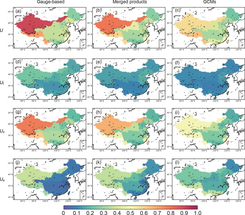
2062                                                 X. Zhou et al.: Uncertainty estimation approach with multiple datasets

ous purposes (Phillips and Gleckler, 2006; Tapiador et al.,
2012; Beck et al., 2017; Sun et al., 2018). As a result, there
are differences between the various products due to measure-
ment errors, model biases, or chaotic noise. The uncertainty
is thus regarded as the deviation of these model results from
their real values.
   However, the real values are difficult to measure and the
uncertainties are difficult to remove from the datasets. Thus,
using ensembles consisting of multiple datasets to generate a
weighted average has become very popular in climate-related
research. The ensemble means of multiple datasets are con-
sidered more reliable estimates than a single dataset. For ex-
ample, IPCC uses 42 CMIP5 (Coupled Model Intercompar-
ison Project Phase 5) models to show historical temperature
changes and 39 CMIP5 models to average future tempera-
ture projections in a RCP 8.5 scenario (Fig. SPM.7 in IPCC,
2013b). Schewe et al. (2014) use nine global hydrologi-
cal models to evaluate global water scarcity under climate         Figure 1. Two classic uncertainty assessments in the current litera-
                                                                   ture: the temporal evolution of the model uncertainty (flowcharts in
change. GLDAS (Global Land Data Assimilation System)
                                                                   red) and the spatial distribution of the model uncertainty (flowcharts
involves four different land surface models (Rodell et al.,
                                                                   in blue). Each of these uncertainty estimates was averaged over one
2004) and GRACE (Gravity Recovery and Climate Exper-               of the dimensions, either space or time, which will lead to loss of
iment) provides estimates from three independent institutes        information about the corresponding dimension.
(Landerer and Swenson, 2012). Using multiple datasets re-
duces the dependence on a single dataset and eliminates the
random variations associated with biases or noise in each sin-
gle model estimate.                                                tainty increases in future projections because of the increas-
   Along with the ensemble means, uncertainty information          ing spread of model estimates (Fig. SPM.7 in IPCC, 2013b),
is recommended to be presented because the level of uncer-         indicating a decreasing consistency but increasing variation
tainty determines the reliability of the ensemble results. In      across various datasets.
general, uncertainties can be quantified as the range of maxi-        The two kinds of ways can easily show the spatial dis-
mum and minimum values (i.e. Vmax −Vmin ), the value differ-       tribution or the temporal evolution of the uncertainty. But a
ence at different quantiles (e.g. V5 % −V95 % ), the consistency   shortcoming is apparent, as the variation along one dimen-
of models (ratio of models following a certain pattern to the      sion (time or space) has to be collapsed to generate the mean
total number of models), the variation (σ 2 ) or the standard      values when we attempt to assess the uncertainty for the other
deviation (σ ) of multiple model estimations. These metrics        dimension (space or time). For example, the averaging over
describe the differences between multiple model estimates in       a specific region to obtain the spatial mean is estimated at
different aspects. Among the metrics, the standard deviation       each time step before obtaining the temporal evolution of the
(σ ) is the most used because it has the same unit as the orig-    model uncertainty (red flowcharts in Fig. 1). In contrast, av-
inal dataset. Moreover, it is less sensitive to extreme samples    eraging over a certain temporal period to obtain the tempo-
and to the number of datasets used for the investigation. The      ral mean is necessary for each grid cell when estimating the
ratio of the standard deviation (σ ) to the mean value (µ),        spatial variations of model uncertainties (blue flowcharts in
the so-called coefficient of variance (CV), representing the       Fig. 1). The averaging, in either dimension, means a loss of
dispersion or spread of the distribution of various ensemble       information about the variation in the data. Any changes in
members (Everitt, 2013), is a unitless value which also shows      the variation that leave the mean values unchanged will not
the degree of uncertainty efficiently.                             be propagated to the global uncertainty estimation. The re-
   Depending on the purpose of data evaluation, the uncer-         sult of this is that the variations between datasets are not fully
tainty between the datasets can be displayed or visualized in      considered when estimating the uncertainties. In other words,
space to show the spatial heterogeneity. For example, the pre-     neither of the uncertainty estimates can represent the whole
dicted future temperature increase has a higher significance       of the differences between multiple datasets. The uncertainty
in different models in the northern high latitudes than in the     can be underestimated, and the similarity of the datasets thus
middle latitudes (Box TS.6 Fig. 1 in IPCC, 2013a). Another         overestimated. Indeed, the current literature has not paid at-
typical implementation is to evaluate the evolution of the un-     tention to the neglect of variation after averaging as well as
certainty over time. In general, the range of the uncertainty      its influence on the assessment of the uncertainty.
decreases in the historical period over time because more             The total variation across multiple datasets is contributed
observations have been accessible recently. But the uncer-         by the spatial heterogeneity, temporal variability and the

Hydrol. Earth Syst. Sci., 24, 2061–2081, 2020                                     www.hydrol-earth-syst-sci.net/24/2061/2020/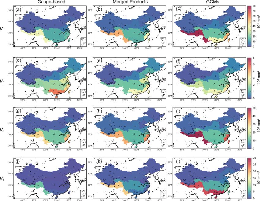
X. Zhou et al.: Uncertainty estimation approach with multiple datasets                                                           2063

model uncertainties. To some degree, the model uncertainty         dimensions of (1) time with a regular time interval (e.g.
is similar to other dimensions as a variation along a third        monthly or annual), (2) space with regular spatial units, with
dimension (ensemble dimension). The key to evaluating the          all the grids re-organized into one dimension from the orig-
model uncertainty is to decompose the variation caused by          inal longitude–latitude grids, and (3) ensemble as the third
differences between the datasets from the other two con-           dimension describing the different ensemble datasets. Thus,
tributors. Although decomposing the variation by means of          the dataset array can be re-organized to be
ANalysis Of VAriance (ANOVA) is often seen in hydro-
                                                                   Z = [zij k ],                                                  (1)
meteorological studies, this is designed to separate the pro-
cess uncertainties generated in different model processes          with the ith time step (i = 1, 2, . . ., m), j th grid (j =
that propagate to the final variation. For example, Déqué          1, 2, . . ., n), and kth ensemble member or ensemble model
et al. (2007) decomposed the uncertainties of regional cli-        (k = 1, 2, . . ., l).
mate models (RCMs) into four sources of uncertainty: sam-             We define the three dimensions to be time, space and en-
pling uncertainty, model uncertainty, radiative uncertainty        semble dimension, and the means for these three dimensions
and boundary uncertainty. Bosshard et al. (2013) decom-            to be the temporal mean, spatial mean and ensemble mean.
posed the uncertainty in river streamflow projections to un-       The corresponding variances are referred to as the temporal
certainties from climate models, statistical post-processing       variance, spatial variance, and ensemble variance. We also
schemes and hydrological models. These implementations             define the grand mean (µ), grand variance (σ 2 ) and total
differ from the purpose of the present study because they fail     sum of squares (SST) (or total variation) across the entire
to separate the uncertainties from the spatiotemporal varia-       database:
tions because spatiotemporal averaging was already applied              m X
                                                                          n X
                                                                            l
in the estimation process. Sun et al. (2010, 2012) for the first
                                                                        X
                                                                   µ=                     zij k /(mnl)                            (2)
time decomposed the total variation into temporal variation             i=1 j =1 k=1
and spatial heterogeneity. They concluded that the variations           SST
along the spatial dimension contributed more to the total vari-    σ2 =                                                           (3)
                                                                        mnl
ation than did the temporal variabilities. However, their ap-
                                                                          m X
                                                                            n X
                                                                              l
proach is only valid for one single dataset and is thus not able   SST =
                                                                         X
                                                                                (zij k − µ)2 .                                    (4)
to evaluate the uncertainties if multiple datasets describe the            i=1 j =1 k=1
same variable. But a generalized approach should be based
on Sun’s work, as one more dimension can be added for a            The total variation receives contributions from the variations
specific analysis of the uncertainties.                            along all three dimensions (Eq. 4). It can be reformulated as
   In the present study, we aim to introduce a new approach to     an expression in terms of the variations along each of the
estimating uncertainty of multiple datasets. The new uncer-        three different dimensions. For instance, the derivation of the
tainty metric should avoid any averaging over time or space,       total variation can start from the third ensemble dimension.
so that all information along each of these two dimensions         For a specific kth ensemble
                                                                                        P Pmember,            the grand mean is for-
can be maintained for the assessment of the uncertainty. Mul-      mulated as µts [k] = m        n
                                                                                           i=1 j =1  z ij k /(mn),  leading to the to-
tiple precipitation products will be used to display the results   tal sum of squares being rewritten as
and explain the specifics of the new approach. In Sect. 2,                 m X
                                                                           X n X
                                                                               l
the details of the three-dimensional variance partitioning ap-     SST =         (zij k − µts [k] + µts [k] − µ)2 .               (5)
proach are introduced. The characteristics of multiple pre-                i=1 j =1 k=1
cipitation datasets and estimations of two other classic un-
                                                                   The SST can be further expanded and rearranged as
certainty metrics are shown in Sect. 3. The results of the new
approach for precipitation products are discussed in terms of              m X
                                                                           X n X
                                                                               l
the types of precipitation datasets in Sect. 4. The differences    SST =         (zij k − µts [k])2
between the new uncertainty estimate and two selected clas-                i=1 j =1 k=1
sic metrics used in uncertainty analysis are analysed and dis-                       l
                                                                                     X               m X
                                                                                                    X n
cussed in Sect. 5. A discussion and some conclusions follow                +2×         (µts [k] − µ)     (zij k − µts [k])
in Sect. 6.                                                                          k=1                     i=1 j =1
                                                                                                         |              {z   }
                                                                                                                        =0
                                                                              m X
                                                                             X n X
                                                                                   l
2     Method and datasets                                                  +         (µts [k] − µ)2 ,                             (6)
                                                                                   i=1 j =1       k=1
2.1    Mathematical derivation                                                |      {z
                                                                                    =mn
                                                                                              }

                                                                           m X
                                                                             n X
                                                                               l                         l
Multiple datasets recording the same climatic variable should
                                                                           X                             X
                                                                   SST =         (zij k − µts [k])2 + mn   (µts [k] − µ)2 , (7)
be reorganized into a three-dimensional database, using the                i=1 j =1 k=1                             k=1

www.hydrol-earth-syst-sci.net/24/2061/2020/                                         Hydrol. Earth Syst. Sci., 24, 2061–2081, 2020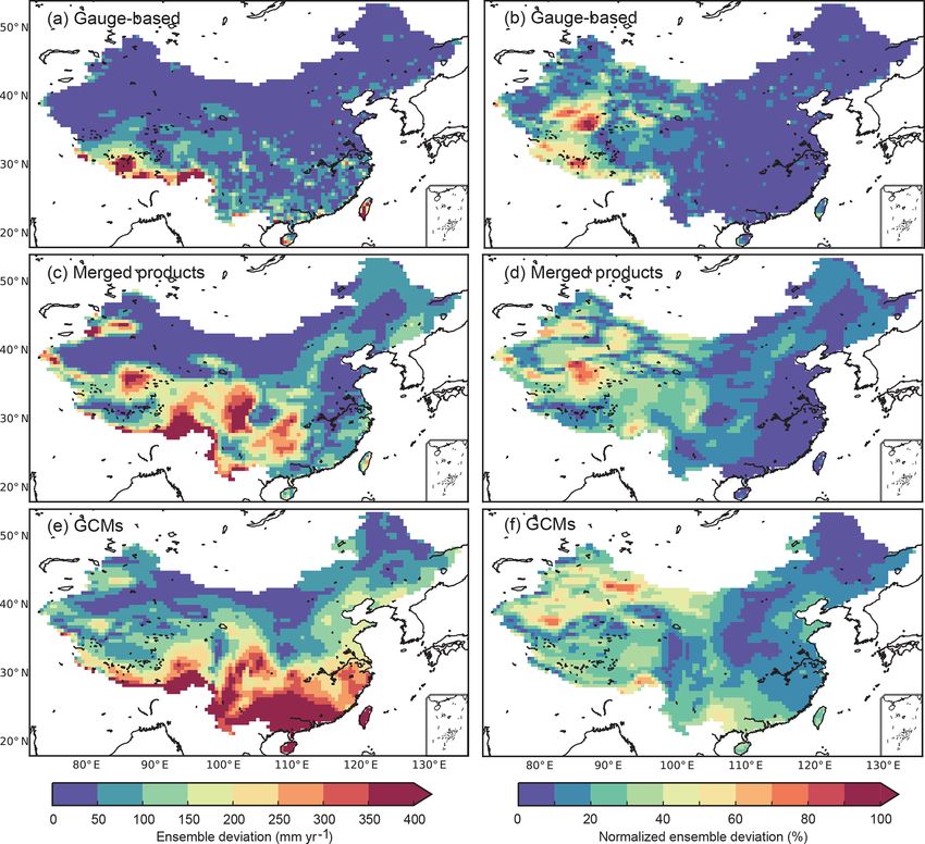
2064 X. Zhou et al.: Uncertainty estimation approach with multiple datasets
l X n
m X
(Zij k − µs [k, i])2
X
SST = mn σts2 [k] + mnlσ 2 (µts ), (8) SST[k] =
k=1 i=1 j =1
m
X
where σ 2 (µts ) is the variation of the grand mean for each en- +n (µs [k, i] − µts [k])2 , (15)
semble member and σts2 [k] is the grand variance in the spatial i=1
and temporal dimensions for the ensemble member k. More- Xm
over, σts2 [k] can be split using the mean of the spatial variation SST[k] =n σs2 [k, i] + nmσ 2 (µs [k, :])
i=1
at each time step σs2 [k, :] and the variation of the spatial mean
σ 2 (µs [k, :]), denoted as in Eq. (9) with its derivation given in = nmσs2 [k, :] + mnσ 2 (µs [k, :]). (16)
Eqs. (10)–(17).
The grand variance of this specific dataset is Eq. (17) (iden-
tical to Eq. 9).
σts2 [k] = σs2 [k, :] + σ 2 (µs [k, :]). (9)
SST[k]
For a specific dataset k, the grand mean µts [k] at the spa- σts2 [k] = = σs2 [k, :] + σ 2 (µs [k, :]) (17)
mn
tiotemporal scale is
Here, σs2 [k, :] is the mean of the spatial variation at each time
m X n step and σ 2 (µs [k, :]) is the variation of the spatial mean, or if
1 X
µts [k] = zij k . (10) we started the derivation from the time dimension, the grand
mn i=1 j =1
variance can be split using the average of the temporal vari-
The total sum of squares of the differences from the grand ation from all regions σt2 [:, k] and the spatial variation of the
mean of this ensemble member is temporal mean σ 2 (µt [:, k]):
m X
X n σts2 [k] = σt2 [:, k] + σ 2 (µt [:, k]). (18)
SST[k] = (zij k − µts [k])2 (11)
i=1 j =1 With Eqs. (9) or (17) and (18), we obtain
1
and the grand variance σts2 is σts2 [k] = [σ 2 (µt [:, k]) + σs2 [k, :]] + [σ 2 (µs [k, :]) + σt2 [:, k]] . (19)
2
m X n
1 X Substituting Eq. (19) into (8) results in
σts2 [k] = (zij k − µts [k])2 . (12)
mn i=1 j =1 l
mn X
SST = [σ 2 (µt [:, k]) + σs2 [k, :]]
The derivation can start from either the spatial dimension or 2 k=1
the temporal dimension. If the derivation starts from the spa- mn Xl
tial dimension, Eq. (11) can be rewritten by
Pincorporating the + [σ 2 (µs [k, :]) + σt2 [:, k]]
2 k=1
spatial mean of each time step µs [k, i] = lj =1 zij k /n:
+ mnlσ 2 (µts ). (20)
m X
X n
2
SST[k] = (zij k − µs [k, i] + µs [k, i] − µts [k]) . (13) The first term on the right-hand side of Eq. (20) can be
i=1 j =1 transformed to
l 2
This can be expanded and then rearranged as σs_t + σs2
mn X
[σ 2 (µt [:, k]) + σs2 [k, :]] = mnl , (21)
m X
n
2 k=1 2
X
SST[k] = (Zij k − µs [k, i])2
2 is the mean value across ensemble members of
where σs_t
i=1 j =1
m
X the spatial variation of the temporal mean, and σs2 represents
+2× (µs [k, i] − µts [k]) the grand mean of σs2 , which is the grand variance across the
i=1 temporal and ensemble dimensions. Eq. (20) then becomes
n
X
× (Zij k − µs [k, i]) 2 +σ2
σs_t
2
σt_s + σt2
s
j =1 SST = mnl + mnl
| {z } 2 2
=0
n X
X m
+ mnlσe2 (µts ), (22)
+ (µs [k, i] − µts [k])2 , (14) 2 denotes the mean value across ensemble members
j =1 i=1 where σt_s
of the temporal variation of the spatial mean, σt2 denotes the
| {z }
=n
Hydrol. Earth Syst. Sci., 24, 2061–2081, 2020 www.hydrol-earth-syst-sci.net/24/2061/2020/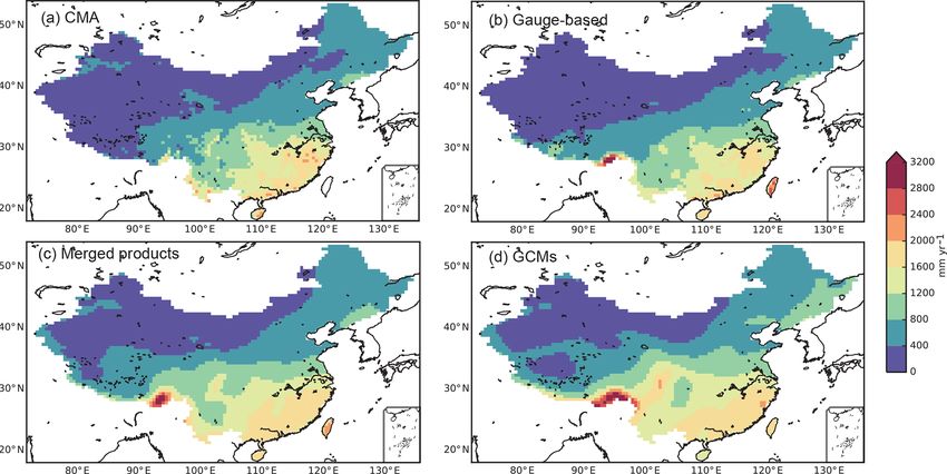
X. Zhou et al.: Uncertainty estimation approach with multiple datasets 2065
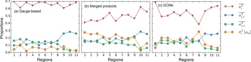
grand mean of σt2 , the grand variance across space and en- 2 , zone C6) and the grand variance of the spa-
tial mean (σe_s
semble dimensions, and σe2 (µts ) denotes the variation across tiotemporal mean for a single ensemble member (σe2 (µts ),
ensemble members of the spatial–temporal means µts . zone F3). Similarly, the other variances only rely on the vari-
Similarly, the global derivation of SST can start from any ances in the corresponding dimension, which shows the inde-
of the other two dimensions (i.e. space or time). This deriva- pendence of the three dimensions. This also is an illustration
tion can then be formulated as of the fact that the uncertainty across ensemble members is
2 similar to the temporal variation and spatial heterogeneity.
σs_e + σs2
2
σe_s + σe2
SST = mnl + mnl
2 2 2.2 Definitions of the metrics for model uncertainty
+ mnlσt2 (µse ), (23) Although the total variation is a result of contributions from
2
σe_t + σe2
2
σt_e + σt2
the spatial heterogeneity, temporal variability and the uncer-
SST = mnl + mnl tainties across different datasets, we mainly focus on the vari-
2 2
ance in the ensemble dimension because the spatial or tempo-
+ mnlσs2 (µet ), (24) ral variation is natural for climatic variables. The uncertainty
of ensemble members is normalized as the ratio of the square
where each variable is defined in Appendix A. Averaging root of the ensemble variance (Ve ) to the grand mean value
these three expressions of SST defined in Eqs. (22)–(24) of the datasets (µ).
leads to p
"
2 +σ2
# Ue = Ve /µ (27)
mnl σt_s t_e
SST = + σt2 + σt2 (µse )
3 2 Two classic metrics used for uncertainty estimates are also
" # introduced for comparison. For each basic spatial unit (in
2 +σ2
mnl σs_t s_e the present study this means a grid cell), we can estimate
+ + σs2 + σs2 (µet )
3 2 the temporal mean of the target variable in each ensemble
" # dataset as µt [j, k], j = 1, . . ., n represents the spatial unit and
2 +σ2
mnl σe_t e_s 2 k = 1, . . ., l represents the index of the dataset. Then we can
+ + σe2 + σe (µts ) . (25)
3 2 estimate the variations across different ensemble datasets of
the mean values as σ 2 (µt [j, :]) (expressed as σe_t 2 [j ] in this
With the total number of degrees of freedom being m × 2
study). The spatial distribution of the σe_t shows the magni-
n × l, the grand variance is expressed as tude of the model uncertainty over space and its root σe_t [j ]
is the model deviation at each spatial unit. The estimate of
2 +σ2
1 σt_s t_e this model deviation over the entire region can be expressed
σ2 = [ + σt2 + σt2 (µse )]
3 2 as
| {z }
Vt
v
u1 n 2
q u X
2 /µ = 1
1 2 +σ2
σs_t N.s.std = σe_t t σ [j ]. (28)
+ [
s_e
+ σs2 + σs2 (µet )] µ n j =1 e_t
|3 2 {z }
Vs 2 [j ] (j = 1, . . ., n) can take a differ-
For each spatial unit, σe_t
2 +σ2
1 σe_t ent value. The values for all the grid cells are averaged to
e_s
+ [ + σe2 + σe2 (µts )], (26) 2 , which shows the general magnitude of the en-
obtain σe_t
3 2
| {z } semble variation over space. The quantity N.s.std is normal-
Ve
ized
q as the ratio of the square root of the averaged variations
where Vt , Vs and Ve denote the temporal, spatial and ensem- 2 to the grand mean of all the datasets µ.
σe_t
ble variances, respectively. An illustration of the present ap- Similarly, the model uncertainty can be normalized as the
proach is shown in Fig. 2 to facilitate the understanding of the ratio of the square root of the averaged ensemble variation
partitioning results. The original database, consisting of mul- 2 to the entire means:
but at different time steps σe_s
tiple datasets, is re-organized into three dimensions (grey in
the centre). Zones with different colours represent different v
u m
1 u1 X
q
processes of the original database from different dimensions 2
N.t.std = σe_s /µ = t σ 2 [i], (29)
(see the details in the caption of Fig. 2 and Appendix A). µ m i=1 e_s
Note that the ensemble variance Ve in Eq. (26) is a com-
bination of several variations across the ensemble members. where σe_s2 [i] (i = 1, . . ., m) is the variation across different
The four components are the variations of temporal and spa- datasets of the spatial means of each product at each time
2 , zone C5), spa-
tial values (σe2 , zone B3), temporal mean (σe_t unit µs [i, k], (i = 1, . . ., m, k = 1, . . ., l).
www.hydrol-earth-syst-sci.net/24/2061/2020/ Hydrol. Earth Syst. Sci., 24, 2061–2081, 2020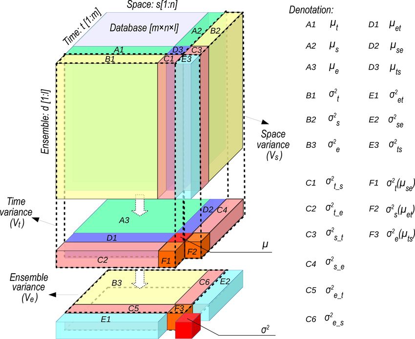
2066                                                     X. Zhou et al.: Uncertainty estimation approach with multiple datasets

Figure 2. Partitioning the temporal–spatial-ensemble variance. The original database is re-organized into three dimensions: time, space and
ensemble. Zones with different colours represent different processes based on the original database through different dimensions. The labels
of the zones are listed on the right; detailed definitions can be found in Appendix A. The grand variance is σ 2 and the grand mean is µ.
The subscripts t, s, and e indicate dimensions of time, space and ensemble, respectively. In Zone A, µx shows the mean values across the
x dimension (x = t, s or e); in Zone B, σx2 indicates the variation across the x dimension; in Zone C, σx_y
                                                                                                          2 indicates the variation across the

x dimension of µy (y = t, s or e); in Zone D, µxy indicates the means across the x and y dimensions; in Zone E, σxy  2 indicates the variation
                                             2
across the x and y dimensions; in Zone F, σx (µyz ) indicates the variation across the x dimension of the means across the y and z dimensions
(z = t, s or e).

   The two uncertainty estimates (Eqs. 28 and 29) correspond
to the two classic metrics presented in the Introduction. We
will compare Ue estimated by the newly proposed approach
with these two classic metrics (N.t.std and N.s.std) to show
their relations and differences.

2.3    Study area and data description

Mainland China has been selected as the study area be-
cause of its large area and different types of climate (Kot-
tek et al., 2006). Ten different subregions have been de-                Figure 3. Ten subregions are defined in this study. These subregions
fined to facilitate the comparisons and analysis of the strong           are mainly river basins (Regions 1–8), but 9 is Southwest China and
spatial variations. The subregions are (1) Songhua River                 10 is Northwest China. Region 11 is the entirety of the Chinese
Basin, (2) Liao River Basin, (3) Hai River Basin, (4) Yellow             mainland.
River Basin, (5) Huai River Basin, (6) Yangtze River Basin,
(7) Southeast China, (8) South China, (9) Southwest China,
and (10) Northwest China; see Fig. 3. The entire Chinese                 longitude–latitude grids or those based on administrative re-
mainland is numbered as the 11th region. Most of the sub-                gions.
regions are natural river basins: this definition is more ap-
propriate for water resource analysis than definitions using

Hydrol. Earth Syst. Sci., 24, 2061–2081, 2020                                           www.hydrol-earth-syst-sci.net/24/2061/2020/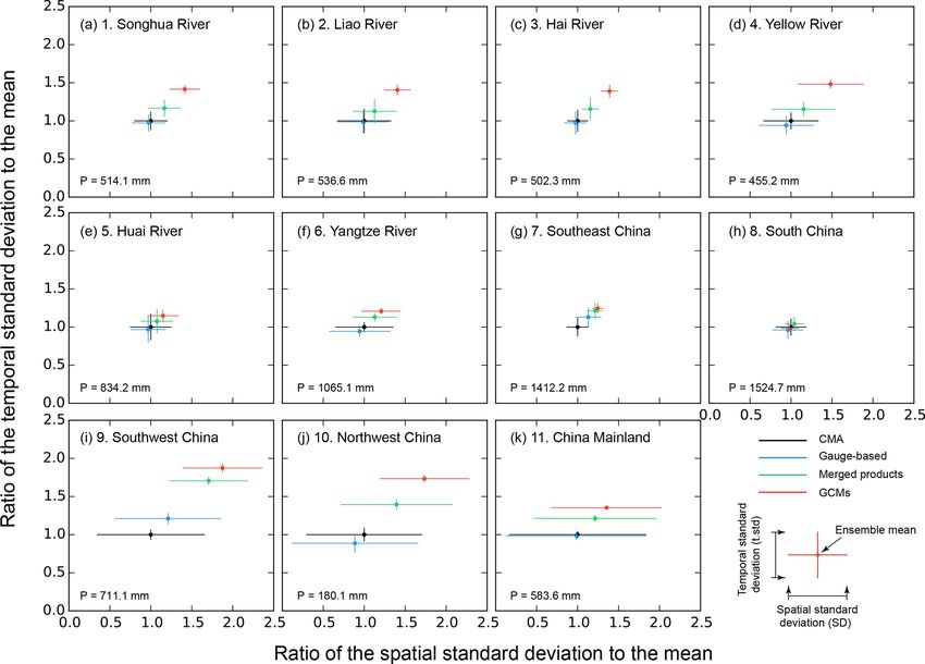
X. Zhou et al.: Uncertainty estimation approach with multiple datasets                                                     2067

   Precipitation is one of the climatic variables sensitive        time steps (daily or monthly) and the overlap time span of all
to large-scale atmospheric cycles and the local topogra-           the datasets is from 1979 to 2005 for all the products.
phy. Thirteen different precipitation datasets from various
sources have been collected for comparison (Table 1). These
datasets have been categorized into three groups according to      3     Characteristics of precipitation and model-quantified
the methods they used for generating the products, namely,               uncertainties with classic metrics
gauge-based products, merged products and general circu-
                                                                   3.1    Spatial patterns of annual precipitation
lation models (GCMs). The gauge-based products (namely,
CMA, GPCC, CRU, CPC and UDEL) use data observed                    The long-term annual mean precipitation (1979–2005) ob-
from global precipitation gauges. The density of the ground        tained by averaging the precipitation from multiple datasets
observation gauges, the representativeness of the gauges, and      in the corresponding precipitation group is mapped in Fig. 4.
the interpolation algorithms for converting the gauge obser-       The annual mean precipitation obtained from the CMA
vations to a gridded dataset differ from product to product.       dataset is 589.8 mm yr−1 (1.6 mm d−1 ) over the entire Chi-
The CMA (China Meteorological Administration) dataset              nese mainland. The gauge-based precipitation has the least
has the densest distribution of gauges and probably has the        bias (−4.1 mm yr−1 , −0.7 % in percentage) compared to the
best quality to capture the spatiotemporal variations of the       CMA precipitation. The precipitation in the merged prod-
precipitation over the study area. The CMA dataset is ex-          ucts and GCMs is larger than that of the CMA by 63.1
cluded when estimating the uncertainty of the gauge-based          and 232.0 mm yr−1 (with the bias equal to +10.7 % and
products: it is chosen as the reference dataset for compari-       +39.3 %), respectively.
son.                                                                  The spatial pattern of the annual precipitation shows a de-
   As for the merged precipitation products, the CMAP,             creasing gradient from Southeast China (> 1600 mm yr−1 )
GPCP and MSWEP use different sources of precipitation              to Northwest China (< 400 mm yr−1 ) in CMA and all other
data (namely, gauge observations, satellite remote sensing,        three precipitation groups. However, they have different abil-
and atmospheric model re-analysis). These different precip-        ities to display the spatial gradient of the precipitation in
itation sources are averaged using different weights. Thus,        some detail. For instance, abrupt precipitation changes rather
the differences between the three merged products are asso-        than following the general gradient occur in some areas in
ciated with the precipitation sources and the weight of the        CMA. This is probably caused by the sudden changes in to-
gauge observations. ERA-Interim is a re-analysis product: it       pography (e.g. the northern Tienshan Mountains, the Qilian
uses near-real-time assimilation with data from global ob-         Mountains), which is not captured in the gauge-based prod-
servations (Dee et al., 2011). Thus, the forecasting model is      ucts because some of the key gauges are not included in the
constrained by the observations and forced to follow the real      production of the gauge-based products. The abrupt changes
system to some degree. Because of its use of observations,         can be somehow represented by merged products and GCMs
ERA-Interim also belongs to the category of merged prod-           because the local variation due to topographic changes can be
ucts.                                                              observed by other measurements or modelled by algorithms.
   GCM precipitation is a pure model estimation because ob-        The precipitation in the merged products and the GCMs is
servations are not used to constrain the simulations. The im-      higher than that of CMA in the Himalayas, and particu-
plemented physical and numerical processes will affect the         larly the GCMs show higher precipitation in the North Tibet
accuracy of the model results. The lack of constraints on the      Plateau as well as the southern part of the Hengduan Moun-
GCMs will cause them to not follow the actual synoptic vari-       tains. These differences show the general characteristics of
ability and explore other trajectories in the solution space.      the three types of precipitation products.
Kay et al. (2015) repeatedly ran the same GCM with a very
small shift in the initial conditions. But the small difference    3.2    Spatial distribution of model uncertainties
leads to an increasing spread in the model outputs after a
number of running time steps (see Fig. 2 in Kay et al., 2015).     In addition to the precipitation differences in its long-term
Therefore, the uncertainty in GCMs can be attributed to the        annual means, differences can be found between datasets
differences in the model structures, parameter settings, and       within the same precipitation group. The spatial distribution
the initial conditions as well. There are more than 20 kinds       of the model uncertainty for each precipitation group, which
of different GCMs; only 4 of them have been chosen, ran-           is expressed as the ensemble deviation of the annual pre-
domly, to maintain the same number of datasets using the           cipitation from different precipitation products, is mapped in
gauge-based products as those using merged products.               Fig. 5.
   All the products of the three precipitation types, including       The ensemble deviation of the datasets based on gauge
CMA, are in gridded format. Although they differ in their          observations is small in most of the land area of China
original spatial resolution, all the products have been inter-     (< 50 mm yr−1 , Fig. 5a). Although the deviation is higher in
polated to a 0.5◦ spatial resolution to unify the spatial units.   the south of China (50–100 mm yr−1 ), the area is not con-
Annual average values are summed based on their original           tinuous in space. The highest deviation occurs along the

www.hydrol-earth-syst-sci.net/24/2061/2020/                                      Hydrol. Earth Syst. Sci., 24, 2061–2081, 2020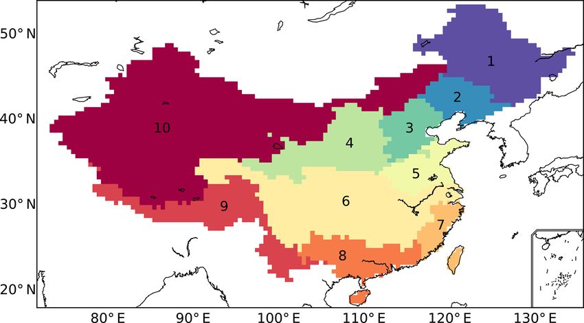
2068                                                    X. Zhou et al.: Uncertainty estimation approach with multiple datasets

Figure 4. Annual precipitation over a long-term period (1979–2005) for each group of precipitation datasets. (a) Annual precipitation of the
CMA dataset, (b) ensemble means of the annual precipitation over the precipitation products in gauge-based precipitation excluding CMA,
(c) ensemble mean of the annual precipitation of all merged products, and (d) ensemble means of the annual precipitation of all GCMs. The
observations in Taiwan are not released in the CMA dataset.

Himalayas, indicating a high variation across the observed              the northeast and part of central China features small uncer-
datasets. Regarding the merged precipitation products, the              tainty, less than 10 %, and the deviation ratio rises signifi-
deviation shows high values (> 200 mm yr−1 , Fig. 5c) in                cantly in South China (e.g. the Pearl River basin), which cor-
Southwest China (e.g. the Tibet Plateau, Yunnan Province,               responds to the high standard deviations in the GCMs shown
Guangxi Province). Moderate deviation is found in North-                in Fig. 5e.
east China, North China and Southeast China. The deviation                 The magnitude of the ensemble deviation demonstrates the
of precipitation has a correlation with the topology, which in-         model uncertainty of the different products in the same pre-
dicates that the performances of the technologies used for the          cipitation group and shows the ability to estimate the pre-
merged products are subject to the topologies as well. Com-             cipitation with different methods. For all products, the en-
pared to the gauge-based and merged products, the deviation             semble deviation is relatively larger where the precipitation
of the selected GCMs has the highest value (> 400 mm yr−1 ,             is higher, especially along the mountains and the subtropical
Fig. 5e) in South China, indicating a significant model uncer-          regions. The deviation ratio is higher in Northwest China,
tainty of the annual precipitation between different GCMs.              where the precipitation is among the lowest in China. Par-
   The ratio of the ensemble deviation to the mean value,               ticularly for the gauge-based products, higher ratios occur
which shows the model uncertainty with no units, is very low            where the gauge density is low and the orographic effect is
in East China (< 10 %, Fig. 5b). It is higher in West China,            apparent (e.g. the Tibet Plateau and other mountainous ar-
especially in the Himalayas and the North Tibet Plateau.                eas). For the merged products and the GCMs, the deviation
Similarly to that of the gauge-based products, the uncer-               ratio increases especially in Southeast China, showing de-
tainty of the merged products has higher values in the west             creasing similarities among different precipitation products.
than in the east of China (Fig. 5d). The area with a devia-             Because the deviation ratio has taken into account both the
tion ratio less than 10 % is mainly distributed in Southeast            variation and the means (which may have a systematic bias),
China and is apparently smaller than that of the gauge-based            the deviation ratio is better than the absolute ensemble devi-
products, showing a decreasing similarity among different               ation at representing the uncertainty, and it is the most com-
merged products. The area with a moderate deviation ratio               monly used in geographic studies.
(10 %–40 %) increases compared to that of the gauge-based
products, and the area is mostly in central and western China.          3.3    Temporal evolution of model uncertainties
The uncertainty estimated in the GCMs shows similar pat-
terns in West China to that of the merged products, but with
                                                                        Figure 5 shows the spatial distribution of the ensemble de-
higher magnitudes in East China (Fig. 5f). Only the area in
                                                                        viation of the precipitation products. However, the temporal

Hydrol. Earth Syst. Sci., 24, 2061–2081, 2020                                          www.hydrol-earth-syst-sci.net/24/2061/2020/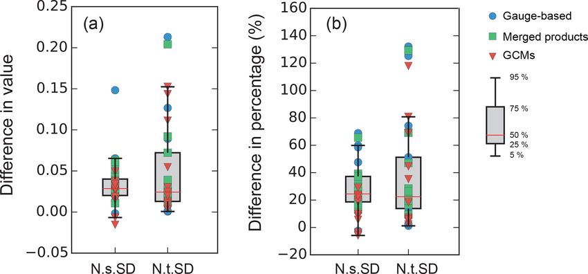
X. Zhou et al.: Uncertainty estimation approach with multiple datasets                                                                     2069

Figure 5. Spatial distribution of model uncertainty in annual precipitation estimated by the ensemble products. The uncertainty is expressed
as the standard deviation of the annual precipitation across ensemble precipitation products of a specific group (a, b: gauge-based products,
middle: merged products, e, f: GCMs). (a, c, e) are the values of the uncertainty. (b, d, f) are the ratios of ensemble deviation to the ensemble
means of the datasets in the corresponding group.

evolution of the deviation, which shows the performance of                 than that of the gauge-based products and merged products
the product over time and its changes, is not captured because             for almost all regions, which agrees with the spatial patterns
the temporal variation has been averaged in order to estimate              in Fig. 4d.
the spatial ensemble deviation in Fig. 5. In this subsection,                 The ensemble deviation across the timescale is shown in
we examine the temporal evolution of the uncertainties in re-              the shaded area in Fig. 6. It is estimated as the deviation
gional annual precipitation estimated by different ensemble                of regional annual precipitation of each product in the same
products. The analysis is based on the 10 subregions defined               group at a specific time step for each subregion. The devi-
in Fig. 3 and the entire Chinese mainland.                                 ation is normalized to facilitate comparisons between dif-
   The annual precipitation of each precipitation group has                ferent subregions. High deviations are found in Southwest
been normalized as the ratio to the long-term annual mean of               China (Fig. 6i) in all three precipitation groups because of
the CMA in each subregion (black line in Fig. 6). The magni-               the large differences along the Himalayas. The deviations
tude of the annual precipitation in the gauge-based products               of the gauge-based products and the merged products in
(the blue solid line) is similar to that of the CMA except in              other regions are small and getting smaller with time. This
Southwest China (Fig. 6i) for the overestimation along the                 is mainly because more observations are included and tech-
Himalayas (Fig. 4a, b). The precipitation in the merged prod-              nologies have improved with time to control the quality of
ucts (the green solid line) is higher in Southwest and North-              the data. A large deviation is found in the merged products
west China, in accordance with Fig. 4c. The annual precipi-                in 10-Northwest China (Fig. 6j) and 4-Yellow River Basin
tation of the GCMs (the red solid line) is apparently higher               (Fig. 6d), where a dry climate dominates and the annual

www.hydrol-earth-syst-sci.net/24/2061/2020/                                               Hydrol. Earth Syst. Sci., 24, 2061–2081, 2020
2070                                                     X. Zhou et al.: Uncertainty estimation approach with multiple datasets

Figure 6. Temporal evolution of the model uncertainty. The uncertainty is expressed as the normalized ensemble deviation of annual precip-
itation across ensemble datasets in each precipitation group for specific subregions. The value on the top right of each panel is the annual
regional precipitation estimated in the CMA dataset (1979–2015). The annual precipitation is normalized as the ratio to the CMA long-term
annual precipitation. The solid curve represents the ensemble mean of precipitation in each precipitation data group over the subregion. The
width of the shaded area represents the standard deviation of the annual precipitation estimated from the datasets within that group for each
year (divided by the annual precipitation of the corresponding group). The shaded area is equally distributed in the two sides of the ensemble
mean values for the corresponding precipitation group.

precipitation is among the lowest. The model deviation of                very different from that of the observations. A smoother re-
GCMs varies between regions as it is at its smallest in 1-               sult is thus obtained when we build the ensemble mean from
Songhua River Basin (Fig. 6a) and 6-Yangtze River Basin                  the GCMs. Unlike the weak variation in GCMs, the gauge-
(Fig. 6f), while it is among the highest in 8-South China                based and merged products have a strong co-variance, and
and West China (9, 10), agreeing with the deviation maps                 the ensemble mean preserves this co-variance.
in Fig. 5.                                                                  For the entire Chinese mainland (Fig. 6k), the ensemble
   Despite their mean values and magnitudes of deviation, the            deviation remains stable in different precipitation groups. In
temporal evolutions of the gauge-based products and merged               contrast, the annual precipitation spans the strongest spatial
products agree well with those of the CMA dataset, while the             heterogeneity in the mainland compared to those divided by
temporal evolution of the members of the category of GCMs                subregions (Fig. 4). However, the spatial variation has been
is weaker and not well correlated with that of the CMA. The              collapsed because the regional precipitation has to be ob-
main reason is that GCMs are not constrained in their synop-             tained before the temporal analysis. It is therefore interesting
tic variability and the sequence of wet and dry years can be             to evaluate how the uncertainty changes when the variations

Hydrol. Earth Syst. Sci., 24, 2061–2081, 2020                                           www.hydrol-earth-syst-sci.net/24/2061/2020/
X. Zhou et al.: Uncertainty estimation approach with multiple datasets 2071
along both the time dimension and the spatial dimension are
Willmott and Matsuura (2012)
considered in the precipitation datasets.
Schneider et al. (2011)
3.4 Variations along the temporal and spatial
Harris et al. (2014) dimensions
Adler et al. (2018)
Zhao et al. (2018)
Beck et al. (2017)
Dee et al. (2011)
Xie et al. (2007)
Xie et al. (2003)
Table 1. Precipitation datasets used in this study. Three different precipitation groups have been identified according to the way the precipitation dataset is generated.
Previous subsections provide the deviation analysis in either
Reference
temporal scale or spatial scale. However, the two are sel-
dom compared with each other. Herein, the standard devi-
ations of the temporal and spatial variations in the precipi-
Climatic Research Unit (CRU)/Ian Harris, Phil Jones, UK
tation datasets are compared in Fig. 7 in 10 subregions and
the World Climate Research Programme (WCRP) and to
Centro Euro-Mediterraneo per i Cambiamenti Climatici,
European Centre for Medium-Range Weather Forecasts, the China mainland for different precipitation groups. The
China Meteorological Administration, Beijing, China
gauge-based products provide similar annual regional precip-
NCEP/Climate Prediction Center, Maryland, USA
the Global Climate Observing System (GCOS)
itation to CMA over the China mainland and the 10 specific
Institut Pierre Simon Laplace, Paris, France subregions except for the region 7-Southeast China (Fig. 7g)
AORI, Chiba, Japan, NIES, Ibaraki, Japan,
Princeton University, Princeton, NJ, USA
University of Delaware, Delaware, USA
and region 9-Southwest China (Fig. 7i), while the merged
Met Office Hadley Centre, Exeter, UK
products provide larger precipitation estimations for most of
GSFC (NASA), Maryland, USA
the regions. It might indicate the degraded ability of remote
NOAA CPC, Maryland, USA
JAMSTEC, Kanagawa, Japan
sensing, one of the important data sources in the merged
products, to estimate the precipitation amount in storms as
the storms mainly contribute to the total precipitation for the
two subregions. The regional precipitation in GCMs is even
larger except in the region 8-South China (Fig. 7h). These
Reading, UK
Lecce, Italy
results indicate the degraded ability of merged products and
Institute
GCMs in reproducing the total value of the annual precipita-
tion.
The spatial standard deviations (as a ratio to the mean) in
University of Delaware Air Temperature & Precipitation
regions 9, 10 and 11 are the largest, indicating the strongest
spatial heterogeneity over these regions. The smallest spatial
Multi-Source Weighted-Ensemble Precipitation
variations are found in regions 7-Southeast China and 3-Hai
CPC Global Unified Gauge-Based Analysis of
China Meteorological Administration dataset
River, either because of the small area or the high homogene-
Global (land) precipitation and temperature
Global Precipitation Climatology Project
Hadley Centre Coupled Model Version 3
Global Precipitation Climatology Centre
ity in these subregions. Nevertheless, the spatial deviation in
CPC Merged Analysis of Precipitation
Climatic Research Unit Time-Series
most of the subregions is larger than the temporal deviation.
The ratio of the temporal deviation to the spatial deviation is
among the smallest in subregions 9, 10 and 11 (k = 0.1, 0.12
and 0.05, respectively; k is the ratio of the temporal devia-
tion to the spatial deviation), showing an apparent difference
Daily Precipitation
between the variations along the two dimensions, while the
difference between the variations along the two dimensions is
ERA-Interim
Long name
small in 3-Hai River basin (k = 1.15) and 7-Southeast China
(k = 0.90), mainly due to the relatively strong variability of
the annual precipitation in different years.
In addition to the differences between regions, the vari-
IPSL-CM5A-LR
ations in different precipitation groups also vary in magni-
CMCC-CM
tude. Excluding the CMA dataset, which consists of only
MIROC5
HadCM3
MSWEP
CRU TS
one single product, the total variation (the sum of the spa-
CMAP
UDEL
ERA-I
GPCC
GPCP
Name
CMA
CPC
tial and temporal variations) across the gauge-based prod-
ucts is higher than that of the other two groups. This differ-
ence demonstrates that the gauge-based products may have
Merged products
the largest spatial variation, and the correlations between the
Gauge-based
different gauge-based products are high, so that this varia-
GCMs
tion is preserved when passing to the ensemble. In contrast,
Type
variations across the GCMs are the smallest, either because
the precipitation estimated in the GCMs is more spatially
No.
10
11
12
13
homogenous than that of other precipitation products or be-
1
2
3
4
5
6
7
8
9
www.hydrol-earth-syst-sci.net/24/2061/2020/ Hydrol. Earth Syst. Sci., 24, 2061–2081, 20202072 X. Zhou et al.: Uncertainty estimation approach with multiple datasets
Figure 7. Spatial standard deviation (horizontal) and temporal standard deviation (vertical) of the annual precipitation across ensemble
datasets in each of the different precipitation groups for each subregion. The P value in the bottom left is the annual precipitation of CMA.
The cross centre represents the long-term means of the regional annual precipitation in ratio to the CMA mean value. The horizontal error
bar represents the spatial standard deviation (spatial variation of the long-term annual precipitation at all the grids). The vertical error bar
represents the temporal standard deviation (temporal variations of region-averaged annual precipitation in different years).
cause the precipitation estimations in different GCMs are not the number of models in each precipitation group (four mod-
consistent in time or space since there are no constraints on els for each of the three groups). Note that the estimated vari-
the GCM simulation. The inconsistent precipitation patterns ance is for a specific subregion because it is an analysis based
will be further eliminated when carrying out an ensemble av- on regions and a long-term scale.
eraging over multiple datasets. The grand variance (V , total value of the variance for all
three dimensions) and its three components (i.e. variance in
time Vt , space Vs and ensemble dimension Ve ) for all the
4 Variances in precipitation products subregions is mapped in Fig. 8. The grand variance is sim-
ilar in space in groups of the gauge-based products and the
4.1 Variances in three dimensions
merged products (Fig. 8a, b, c), while the grand variance in
In the preceding section, we introduced the spatial and tem- the GCMs is larger and is approximately twice the V in the
poral characteristics of the annual precipitation. The varia- other two groups in regions 9-South China and 10-Southwest
tions in the precipitation in two dimensions of the precip- China. The differences are mainly constituted by the spatial
itation products in the same precipitation group were esti- variance and ensemble variance (Fig. 8i, l).
mated by two classic metrics. In this section, we will present The temporal variance Vt is the smallest among all three
the uncertainty results estimated by the newly proposed ap- variances, and it has very little differences in North China
proach to the variance. As introduced in the Methods section, (Fig. 8d, e, f). But it is higher in the gauge-based prod-
the input annual precipitation to the approach is re-organized ucts than in the merged products and GCMs in regions 8-
into three dimensions: (1) time, 27 years from 1979 to 2005, Southeast China and 9-South China, indicating a relatively
(2) space, 0.5◦ grids in a specific region, and (3) ensemble, strong temporal variation in the annual precipitation series,
Hydrol. Earth Syst. Sci., 24, 2061–2081, 2020 www.hydrol-earth-syst-sci.net/24/2061/2020/X. Zhou et al.: Uncertainty estimation approach with multiple datasets 2073
Figure 8. Maps of the estimated grand variance (V ) and variances in different dimensions (Vt , Vs , Ve ) across the ensemble datasets in each
of the three different precipitation groups.
in accordance with the larger uncertainty ranges shown in One can conclude that the grand variance and individual
Fig. 6h, i. Similar patterns of the spatial variance Vs are found variance for each of the three different dimensions are gen-
in the gauge-based products and merged products (Fig. 8g, erally larger in the precipitation group consisting of GCMs.
h). The largest Vs is found in regions 7-Southeast River The variations for the gauge-based products and merged
basin and 9-Southwest China because the precipitation sig- products are similar in values and spatial distribution. How-
nificantly varies in space in these two subregions: it is higher ever, in addition to the variances, the deviation defined as
in GCM precipitation especially in 9-Southwest China, in- the ratio of the square root of the variance to the mean (e.g.
dicating the strong spatial heterogeneity in the GCM mod- U , Ut , Us , Ue ) contains extra information about the regional
els over the Himalayas (Fig. 8i). The ensemble variance Ve means and will be discussed in the following section.
is relatively small in most regions for gauge-based products
(Fig. 8j), indicating that the model variation across datasets in 4.2 Deviations in three dimensions
the observation group is small. A similarly small Ve is found
in the northern regions of the merged products as well as in In contrast to the spatial gradient of the magnitude of the
the GCMs for the regions in North China, while the intra- variance distributed over the 10 subregions (Fig. 8), the larger
√
ensemble variations are large in the GCMs, especially in values of the total deviation (U = V /µ) occur in the north-
the south, especially 9-Southwest China and 8-South China west, but a lower value generally occurs in South China
(Fig. 8k, l). (Fig. 9). The decreasing tendency of magnitude of the precip-
itation from the southeast to the northwest results in a shift
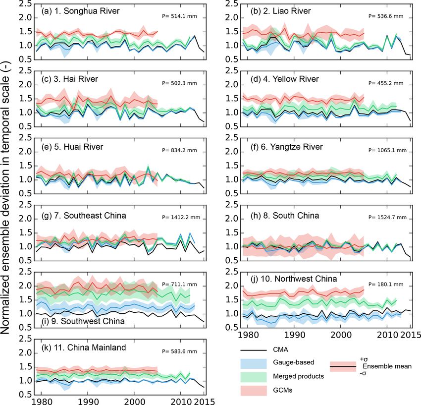
www.hydrol-earth-syst-sci.net/24/2061/2020/ Hydrol. Earth Syst. Sci., 24, 2061–2081, 20202074 X. Zhou et al.: Uncertainty estimation approach with multiple datasets
of the spatial gradient compared to Fig. 4. The total devia- 5 Comparison of the uncertainty Ue with the classic
tion U is highest in Northwest China (U = 0.89, Fig. 9a, b, metrics
c) for all three precipitation groups, but is relatively small
in the northeastern 1-Songhua River (U = 0.27) and 8-South 5.1 Deviation from the classic uncertainty metrics
China (U = 0.29) for the gauge-based products. A relatively
lower U is found in subregion 6-Yangtze River in the merged In this section, we will compare the uncertainty Ue of the
products and GCMs in the eastern part of China. ensemble members estimated by the three-dimensional par-
Deviations along the temporal and spatial dimensions are titioning approach with the two classic metrics defined as
inherent, as they show the temporal evolution and spatial het- N.s.std in Eq. (28) and N.t.std in Eq. (29), to explain how
erogeneity of the precipitation products. The results show these three metrics are related and differ with each other.
that Ut is small and contributes very little to the total U , indi- As shown in Fig. 10, Ue is correlated with both N.s.std and
cating the weak fluctuation of annual precipitation compared N.t.std. The correlation is stronger when Ue is smaller than
to the spatial heterogeneity (Fig. 9d, e, f). The smallest value 0.2, where the regions from 1 to 8 are generally included
of Ut for the GCMs is in accordance with the weakest tempo- for all three precipitation groups. But Ue is in general larger
ral variations in Fig. 6. The deviation in the spatial dimension than N.s.std and N.t.std for the products. This deviation is be-
(Us ) contributes the most to the total deviation, especially in cause the variation along one dimension has been collapsed
Northwest China (Us = 0.77 for the gauge-based products, when calculating the deviation along the other dimension.
Fig. 9g). The high Us indicates the strong spatial heterogene- For subregions 9, 10 and 11, N.s.std and N.t.std deviate the
ity of precipitation in the region, demonstrating that the abil- most from the 1 : 1 line of Ue . Taking subregion 9-Southwest
ity to describe the precipitation varies significantly in differ- China in the gauge-based products as an example, the tem-
ent places in the subregions. However, because the spatial poral variance is 62.4 mm yr−1 , while the spatial variance is
variations obtained by the GCMs in Northwest China are less 571.8 mm yr−1 (Fig. 7i). The difference between N.s.std and
significant than with the other two groups, the value of Us for Ue is 0.058 (= 0.297–0.239; the deviation ratio is 24.3 %)
region 10-Southwest China (= 0.51) is smaller than that of when the temporal variation is collapsed. The difference be-
the gauge-based and merged products. tween N.t.std and Ue is 0.126 (= 0.297–0.171; the devia-
The variations along the temporal and spatial dimensions tion ratio is 73.4 %) when the spatial variation is collapsed.
show the natural precipitation patterns, but the deviation of The deviation is significantly larger than that between Ue and
multiple products (Ue ) shows the ability to consistently rep- N.s.std, showing that the collapse will induce a deviation re-
resent the spatiotemporal patterns. Therefore, Ue indicates lated to the magnitude of the collapsed dimension.
the uncertainty of the ensemble precipitation products in the These subregions (9, 10, 11) feature strong spatial het-
same group. For the gauge-based products, Ue is smaller than erogeneities (Fig. 7i, j, k) in the annual mean precipitation
0.1 for regions in East China, indicating that the model vari- (Fig. 4). The averaging process before estimating the clas-
ations are relatively small compared to the annual means. sic metrics will cause a significant smoothing of the datasets
The value of Ue is higher for 9-Southwest China (= 0.30) when the spatial heterogeneity of the datasets is very strong,
and 10-Northwest China (= 0.37), showing large variations because the spatial variation is significantly higher than the
even in the gauge-based products. For the merged products, temporal variation, as shown in Fig. 7. The estimation of
Ue is similar to that of the gauge-based products in West N.t.std, which needs an averaging over the spatial dimension,
China (= 0.36), while it is larger in the east, especially for 6- will lose more information than that in the time dimension.
Yangtze River and 4-Yellow River (more than 2 times larger The deviation between N.t.std and Ue (Fig. 10b) is larger than
than Ue of the gauge-based products). that between N.s.std and Ue (Fig. 10a). The priority of the
For the GCM precipitation, Ue increases compared to the precipitation types also changes, from model dominated (the
other two groups in the eastern subregions, corresponding to model uncertainties in GCMs are larger than the others) to
the higher spatial model uncertainty in GCMs over the east- region dominated (the uncertainties in the specific regions
ern regions shown in Fig. 5. It decreases in 10-Northwest 9, 10, and 11 are larger than in the other regions no mat-
China (Ue = 0.25), and a possible reason for this is that the ter which precipitation data are used). This indicates that the
spatial homogeneity of the variations in 10-Northwest China difference in model variation over space can be reflected in
(Fig. 5f) is stronger than that of the other groups (Fig. 5b, d, the new uncertainty Ue .
f). In the GCMs, the highest Ue occurs in Southwest China, Each classic metric has its physical meaning: N.s.std rep-
where both the means and the variations are higher (Figs. 4 resents the uncertainties over space and N.t.std represents the
and 5). One can conclude that Ue is linked with the mag- uncertainties across time. The comparison of Ue with each
nitude of the model uncertainties in Figs. 5 and 6, indicating of them demonstrates the metric performance on the same
that it is to some degree correlated with the classic metrics, as physical meaning. It is possible to compare Ue with a combi-
higher Ue covers the grid cells or regions with higher model nation of the two classic metrics, but the combination could
uncertainty. be far more complex than a simple sum of the two classic
metrics. However, a qualitative comparison is accessible be-
Hydrol. Earth Syst. Sci., 24, 2061–2081, 2020 www.hydrol-earth-syst-sci.net/24/2061/2020/You can also read