MIDAS: A New Integrated Flood Early Warning System for the Miño River - MDPI
←
→
Page content transcription
If your browser does not render page correctly, please read the page content below
water
Article
MIDAS: A New Integrated Flood Early Warning
System for the Miño River
Diego Fernández-Nóvoa 1 , Orlando García-Feal 1, * , José González-Cao 1 , Carlos de Gonzalo 2 ,
José Antonio Rodríguez-Suárez 2 , Carlos Ruiz del Portal 3 and Moncho Gómez-Gesteira 1
 1   Environmental Physics Laboratory (EPhysLab), CIM-UVIGO, Universidade de Vigo, Campus As Lagoas s/n,
     32004 Ourense, Spain; diefernandez@uvigo.es (D.F.-N.); jgcao@uvigo.es (J.G.-C.);
     mggesteira@uvigo.es (M.G.-G.)
 2   Tragsatec, SAIH Miño-Sil, 32003 Ourense, Spain; c.gonzaloaranoa@gmail.com (C.d.G.);
     josearsuarez@hotmail.com (J.A.R.-S.)
 3   Confederación Hidrográfica Miño-Sil, 32003 Ourense, Spain; cgruiz@chminosil.es
 *   Correspondence: orlando@uvigo.es; Tel.: +34-988-368-791

 Received: 30 June 2020; Accepted: 15 August 2020; Published: 19 August 2020

 Abstract: Early warning systems have become an essential tool to mitigate the impact of river floods,
 whose frequency and magnitude have increased during the last few decades as a consequence of
 climate change. In this context, the Miño River Flood Alert System (MIDAS) early warning system has
 been developed for the Miño River (Galicia, NW Spain), whose flood events have historically caused
 severe damage in urban areas and are expected to increase in intensity in the next decades. MIDAS is
 integrated by a hydrologic (HEC-HMS) and a hydraulic (Iber+) model using precipitation forecast as
 input data. The system runs automatically and is governed by a set of Python scripts. When any
 hazard is detected, an alert is issued by the system, including detailed hazards maps, to help decision
 makers to take precise and effective mitigation measures. Statistical analysis supports the accuracy
 of hydrologic and hydraulic modules implemented to forecast river flow and flooded critical areas
 during the analyzed period of time, including some of the most extreme events registered in the Miño
 River. In fact, MIDAS has proven to be capable of predicting most of the alert situations occurred
 during the study period, showing its capability to anticipate risk situations.

 Keywords: early warning system; flood; hydrology; HEC-HMS; hydrodynamics; Iber+

1. Introduction
     Flood events have increased both their frequency and intensity during the last few decades [1,2].
This has occurred for multiple reasons, but two are especially remarkable. On the one hand, changes
in land uses, including the increase in urbanization, cause an increase in the run-off volume that can
reach river flow systems [3,4]. On the other hand, changes in precipitation patterns have been induced
by the impact of climate change [5,6]. In fact, one of the most dangerous consequences associated with
climate change is the intensification of extreme rainfall events, increasing the hazard of the associated
flood episodes [7–11].
     Flood events have been estimated as one of the most important natural hazards in recent decades.
These disasters have affected millions of people and caused billions of dollars in losses due to the
damage caused [12,13]. Consequently, the development of early warning systems (EWSs) designed
to forecast flood events has increased during the last few decades [14,15]. Several examples can be
found in the literature. The Hydrometeorological Data Resources and Technology for Effective Flash
Flood Forecasting (HYDRATE) project aims to develop a methodology for flash flood forecasting in
Europe [16], the European Flood Awareness System (EFAS) provides streamflow forecasting with a

Water 2020, 12, 2319; doi:10.3390/w12092319                                    www.mdpi.com/journal/water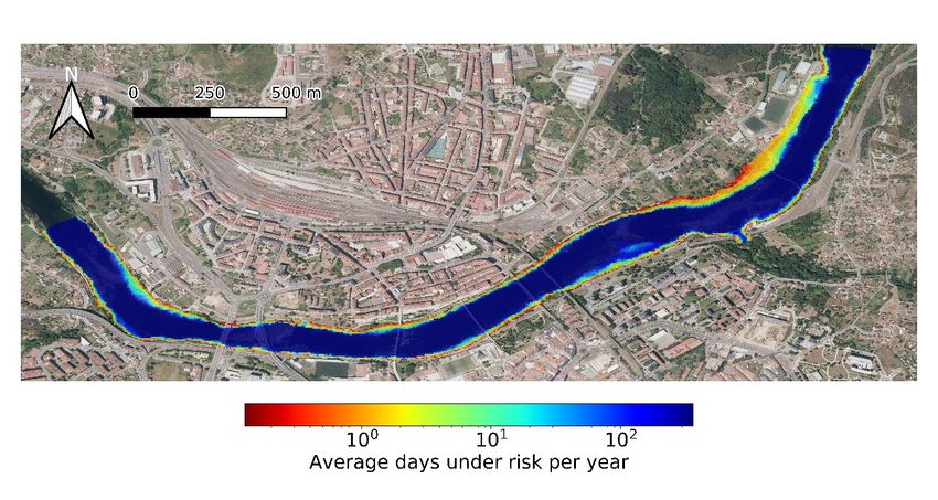
Water 2020, 12, 2319                                                                                 2 of 21

time horizon of 10 days for the European river network [17–20], and the Global Flood Awareness
System (GloFAS) offers a global hydrological forecast [21]. Alfieri et al. [7] also describe several EWS
developed at more local scale in Europe. The reader can find a detailed comparison between two
EWSs applied to a regional scale in Corral et al. [22]. One of them is based on precipitation forecast,
while the other one is based in rainfall-runoff models. Other EWS developed to a regional scale is
EHIMI [22], applied by the Water Agency of Catalonia (ACA) in Spain. Liu et al. [6] shows the rapid
advances in the flood early warning systems development in China, and Hirpa et al. [23] present a
flood forecasting system for the major rivers in South Asia based on satellite data. Other examples
can be found in Cloke and Pappenberger [24] and De Luca et al. [25]. Cloke and Pappenberger [24]
show a review of different approaches of flood forecasting systems based on ensembles of weather
prediction, and De Luca et al. [25] present several mathematical models operating into EWS functioning.
The flood EWS focused on predicting the evolution of river floods, are essential because they allow to
take measures to prevent and mitigate the dramatic consequences that arise in flood scenarios [15].
Therefore, EWSs suppose a useful tool with the potential to save lives, diminish the damage of
fundamental infrastructures and enhance the resilience of the society [12,15,26]. An example of an EWS
focused on the hazard and the personal and economic losses is shown in Ritter et al. [27]. Within this
context, the base of a flood EWS is the hydrological model component, which transforms rainfall in
runoff, which determines the extent of the flood in rain-dominated systems [28,29]. The hydrological
component can be focused on continuous modelling or on single event applications. In the first case,
the continuous schemes are able to reproduce correctly the rainfall-runoff processes along large time
periods, however they depend on multiple variables that should be measured or/and calibrated [8,30].
This can be an important constraint, especially in poorly gauged basins, because the accurate development
of the approach requires a complex data set [30]. The single event approach usually has a lower number of
variables involved and it is only focused on individual and concrete events [29,31]. Although single-event
approaches also need to be calibrated, the need for a lower number of parameters allows the approach to
be applied in a greater number of situations. Taking also into account that EWSs are especially focused
on extreme riverine floods, event-based models have been widely used for runoff calculation in several
engineering applications worldwide, especially the soil conservation service curve number (SCS-CN)
approach [32]. The main advantage of the SCS-CN model lies in its simplicity, which makes it applicable in
a great number of basins, even when data availability is limited.
     Most EWSs report flood hazard based only on the discharge provided by the hydrological model.
However, some EWSs implement a step forward including a hydraulic module [8]. In this case,
the river flow forecasted by the hydrological model is used to feed the hydraulic model. With this, it is
possible to forecast the water depth and velocity throughout the area under interest. Thus, the alert
reports are based on the hazard maps provided by the hydraulic model, which allows a detailed view
of the impact of flood events [8,33]. However, hydraulic models usually require large computational
times, which significantly limits their application in real-time flood forecasting. For this reason, the use
of hydraulic models as part of an EWS is limited [8,33,34].
     The aim of this study is to design an EWS that efficiently combines hydrological and hydraulic
components. In this sense, a novel hydrological methodology was developed. This new technique
allows us to use the SCS-CN method for continuous modelling, bringing together the main advantages
of both approaches (continuous and single event). In addition, the new implementation of the 2D
hydraulic model Iber+ [35] was integrated as part of the EWS. Iber+ is a GPU-parallelized version
of the Iber model [36], which improves the efficiency of the former model in about two orders of
magnitude. This implementation overcomes the limitations of hydraulic models to be used in EWSs
and allows the user to simulate areas under flood risks at a reasonable time [33]. This is especially
suitable for applications where a fast response is crucial.
     The proposed methodology is applied and evaluated in the Miño River (Galicia, northwest Spain)
whose flood events can cause damage in important urban areas [33]. This approach is particularly
helpful for Galicia, where the intensity of extreme rain events is expected to increase in the next decades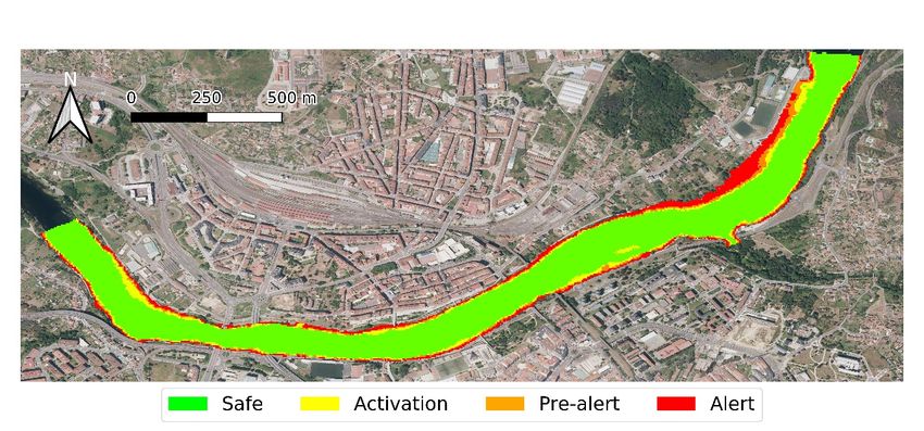
Water 2020, 12, 2319                                                                                3 of 21

due to climate change, leading to hazardous flood episodes [37]. This makes the development of
systems able to accurately predict in advance the flood events occurring in the area under scope even
more necessary.
     The method offers numerous advantages, including ease of application in other areas, especially
in poorly sampled river basins. In turn, the real-time information provided by the hydraulic model
allows us to obtain a better representation and an in-depth knowledge of the impact of river floods.
This information can help decision makers to take suitable measures to mitigate the damage.
     This work is organized as follows: Section 2 presents a brief description of the area under study and
describes in detail the hydrologic and hydraulic models applied in this work. The general architecture
of the EWS and the statistic parameters used to define the accuracy of the EWS are also presented
in this section. The results obtained with both hydrologic and hydraulic models are validated and
analyzed in Section 3. Finally, Section 4 shows the conclusions of this work.

2. Study Area and Methodology

2.1. Study Area
     Figure 1 shows the study area analyzed in this work. This area is located in the NW Iberian
Peninsula occupying a total extent of around 5000 km2 , with an elevation ranging from 90 m.a.s.l.
to 1200 m.a.s.l. (Figure 1a,b). It corresponds to the upper reach of the shared Portuguese–Spanish
Miño River catchment. The Miño River presents a pluvial regime, with maximum river flows during
the winter months and minimum flows during the summer [38]. This flow pattern is regulated by
the precipitation characteristics of the area under scope, characterized by a seasonal evolution of
Azores high and Iceland low, which provokes the occurrence of most of rainy events during the winter
months [39]. Attending to its topographic features, the area under consideration was divided in six
sub-basins for the hydrological procedure (Figure 1b). The outlet of the catchment is located at Ourense
City (Figure 1c–e), which suppose a critical area affected by recurrent floods under extreme conditions.
Attending to these reasons, Ourense is considered to be the test area to analyze the accuracy of the
hydraulic model to reproduce flood events. The area delimited by the red line in Figure 1c corresponds
to the domain of the hydraulic model. The input and output of the domain are also shown in Figure 1c.
The section of the river is 3 km long and the total area is about 1 km2 . More than 50 land uses were
defined attending to the characteristics of the terrain (Figure 1e).

2.2. Description of the Early Warning System

2.2.1. Hydrological Model: HEC-HMS
     The semi-distributed model HEC-HMS [40,41] was used to process the main hydrological features
of the area under scope. This modelling system, which is one of the most used for hydrological
procedures, offers accurate results in locations close to the area under scope [8,31,33]. The designed
methodology only requires the input of a few variables to resolve the hydrologic processes—curve
number (CN), lag time (Tl), baseflow linear reservoir (BLR), and the routing coefficients along the river
channel, as described below.
     Rainfall infiltration is determined using the SCS-CN [42,43]. This procedure only requires the
knowledge of the CN parameter. The standard CN (intermediate or average conditions) for each
sub-basin under scope was firstly calculated following [44,45]:

                                                      25, 400
                                               CN =                                                    (1)
                                                      S + 254

where S is the potential maximum watershed site storage after runoff begins that is computed using:
                                                   q        !
                                                      2
                                     S = 5 P + 2Q − 4Q + 5PQ                                           (2)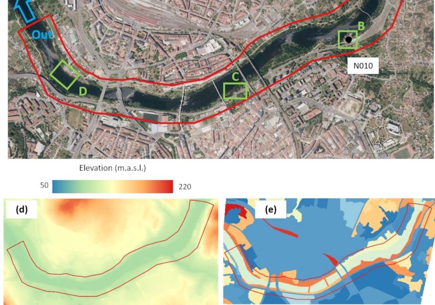
Water 2020, 12, 2319                                                                                                              4 of 21

where Q is the runoff depth and P is the rainfall depth, both obtained from SIMPA (stands for integrated
precipitation-contribution modelling system) model [46]. Equation (2) is also dependent of initial
abstraction, which was simplified as 0.2·S following Stewart et al. [45], resulting in the equation
presented above.
      Water 2020, 12, x FOR PEER REVIEW                                                                                 4 of 21

      Figure  Figure  1. Area
                 1. Area       of study.
                           of study.  (a)(a) locationofofthe
                                           location       theentire
                                                              entire catchment
                                                                     catchmentofofthe shared
                                                                                    the      Portuguese–Spanish
                                                                                        shared   Portuguese–Spanish  MiñoMiño
              River (shaded area) in the Iberian Peninsula and the riverbed (blue line); (b) subbasins (Sb1, Sb2, …,
      River (shaded area) in the Iberian Peninsula and the riverbed (blue line); (b) subbasins (Sb1, Sb2,
              Sb6) of the domain; (c) area of study in Ourense (PNOA courtesy of © Instituto Geográfico Nacional).
      . . . , Sb6) of the domain; (c) area of study in Ourense (PNOA courtesy of © Instituto Geográfico
              Area enclosed by the red line defines the domain of the hydraulic model. The inlet and outlet
      Nacional). Area enclosed by the red line defines the domain of the hydraulic model. The inlet and
              boundaries of the domain and the gauge stations N001 (Lugo) and N010 (Ourense) are also shown.
      outlet    boundaries
              Green  rectanglesofdefine
                                   the domain     andareas.
                                         the control    the gauge
                                                             Controlstations  N001 sport
                                                                      area A: public (Lugo)  and N010
                                                                                          facility; control(Ourense)    are also
                                                                                                            area B: gauge
      shown.      Green   rectangles   define   the control   areas.  Control  area A: public  sport  facility; control
              station N010; control area C: public path; control area D: public thermal baths. The inlet (in blue         area B:
      gauge   arrow) and outlet (out blue arrow) boundaries are also depicted. (d) Topographic features and (e) blue
                station  N010;   control  area  C: public   path;  control area D: public thermal    baths.  The  inlet (in
      arrow)     and
              land    outlet
                    uses      (out
                         of the areablue
                                     underarrow)
                                             studyboundaries
                                                   in Ourense. are also depicted. (d) Topographic features and (e) land
      uses of the area under study in Ourense.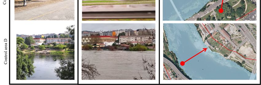
Water 2020, 12, 2319                                                                                  5 of 21

     The theoretical CN value obtained at Lugo was calibrated using river flow data provided by the
Confederacion Hidrografica del Miño-Sil (CHMS, https://www.chminosil.es). The Lugo location was
selected for calibration purposes because the Miño River exists there under natural condition and is
not affected by river structures like dams. This procedure was carried out in order to completely adjust
the CNs characterizing the area under study. The Nelder–Mead algorithm [47] was used to obtain
the optimum value with the Nash–Sutcliffe efficiency index (NSE) as an objective function, which has
reported accurate results in surrounding areas [8]. The results obtained show a close relation between
the theoretical CN value obtained from Equation (1) and the calibrated value (81 and 84, respectively),
which suppose differences of less than 5%. The correction in CN value detected in calibration process
was extrapolated to the rest of the sub-basins. First, theoretical values were calculated by means of
Equation (1), and then, the correction (in percentage) was applied. In all cases, obtained CNs were
rounded to the upper value (Table 1). CN values are similar to the ones obtained in other studies
developed in close areas [31].

                         Table 1. Main hydrological characteristics of the area under scope.

               Subbasin        Area (km2 )     CNdry       CNaverage      CNmoist    Lag Time (min)
                   Sb1            2172           69            84           93             1740
                   Sb2            1219           69            84           93             1500
                   Sb3             897           72            86           94             1620
                   Sb4             255           75            88           95              840
                   Sb5              93           72            86           94              540
                   Sb6             130           71            85           93              600

     In addition, it is a well-known fact that this standard CN should be modified attending to the
different moisture content of the soil [31,48,49]. This means that the antecedent moisture content (AMC)
plays a key role in the rain-runoff processes. The criterion to determine the different conditions is based
on [50], which defines three possible CN classes (dry, average, and moist), whose inter-connections are
specified in the equations defined in [50].

                                                        4.2 × CNaverage
                                         CNdry =                                                         (3)
                                                   10 − 0.058 × CNaverage

                                                         23 × CNaverage
                                         CNmoist =                                                       (4)
                                                      10 + 0.13 × CNaverage
     The thresholds delimiting the corresponding CN class are also based on the SCS criterion [50],
establishing two different annual seasons (non-humid and humid) and a dependence of the cumulative
rainfall occurred in the antecedent days. The SCS approach only takes into account the antecedent
five days for AMC calculations, however, some studies reveal that the rainfall of a larger number of
antecedent days has also an important impact [51,52]. This was also tested in locations close to the area
under scope, where [31] detected the important role of the previous 30 days in the moisture content.
Slightly better results were obtained in the study area when the AMC of the previous 30 days was
considered during the non-humid season and the AMC of the previous 5 days during the humid season
(Table 2). In the present work, the non-humid season was calculated to last from April to November
and the humid season from December to March. However, some false peaks of river discharge can be
obtained in December under the first intense precipitations. To correct this issue, the transition from the
non-humid to the humid season starts only when the 30-day AMC surpasses 216 mm (that corresponds
with the dry conditions threshold for the non-humid season). Taking into account the considerations
commented above, it can be concluded that the conditions that better represent the AMC of the area
under scope are those described in Table 2. The obtained thresholds are in accordance with Cea and
Fraga [31].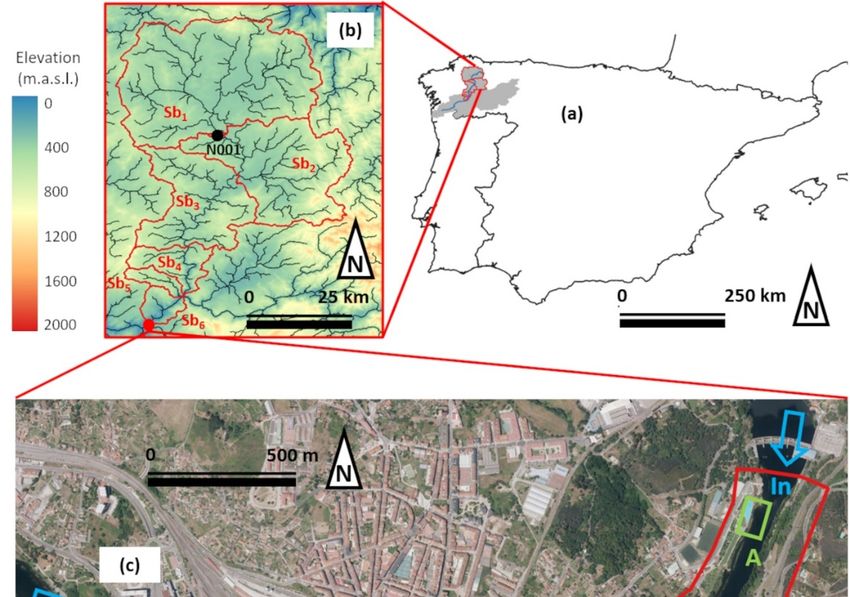
Water 2020, 12, 2319                                                                                     6 of 21

         Table 2. Antecedent moisture content (AMC) conditions representative of the area under scope.

                                       Non-Humid Season                      Humid Season
                   CN Classes       (April–November) (30-day            (December–March) (5-day
                                    Antecedent Rainfall) (mm)           Antecedent Rainfall) (mm)
                        CNdry                  28

     The SCS unit hydrograph was selected to model the transformation of rainfall excess into surface
runoff [43,50]. This approach only requires the input of the Lag Time and has shown accurate results
for nearby areas [8,33]. First, time of concentration was calculated following the equation proposed by
spanish development ministry [53], which provides a good approximation for Spanish basins,

                                           Tc = 0.3 × L0.76
                                                       c    × Jc−0.19                                       (5)

where Tc is the time of concentration in hours, Lc is the length of the longest flow path in kilometers,
and Jc is the slope of the longest flow path in m/m.
     Then, Lag Time was estimated by means of the approximation proposed by the SCS,

                                                Tl = 0.6 × Tc                                               (6)

Tl was calibrated at Lugo station following the procedure explained above, obtaining larger values
than the theoretical ones for our case of study. After the calibration process, the Tl equation which best
represent the area under scope was

                                          Tl = 0.37 × L0.76
                                                       c    × Jc−0.19                                       (7)

      This equation was used for all the sub-basins of the study. Lag time values were rounded at
hourly scale according to the available time data resolution (Table 1).
      Baseflow dynamics was also calibrated at the Lugo station. For that, periods of diminishing flow
after precipitation events were evaluated in order to know the constants associated to baseflow routing.
These periods were selected several days after the precipitation to ensure that most of the river flow
is due to baseflow dynamics. According to previous studies analyzing nearby areas [8], the scheme,
which better represents the baseflow dynamics of the area under study, was a linear reservoir with two
layers, one of them with a faster response (180 h) than the other (600 h). The results obtained were used
for the rest of the sub-basins. Also, it was observed that the baseflow response during the non-humid
season was significantly attenuated compared with the humid season. This fact caused false peak
values associated to precipitation events during dry season. To overcome this issue, a number between
one and three sequential reservoirs was used depending on the average river flow in the previous
30 days. This approach achieves an attenuation in the baseflow response in concordance with the
observed river flow.
      Regarding the channel routing, the Muskingum–Cunge method [54] was selected, which has
provided accurate results in previous studies in close areas [33]. The variables required (river length,
slope, width, etc.) were determined according to data obtained from digital terrain models.
      Finally, it is important to take into account that the most important tributary of Miño River, the Sil
River, is not simulated. This simulation of Sil River flow is not straightforward since the river is highly
regulated by a network of connections among dams. However, the Sil River debouches into the Miño
River upstream from the city of Ourense, which makes it mandatory to forecast its contribution at
that location. To overcome this limitation, the river flow predicted by the hydrological system in
Ourense is reconstructed. For that, the system analyzes the relation between simulated river flow
(which considers only Miño catchment) and the real flow observed at that location (which also includes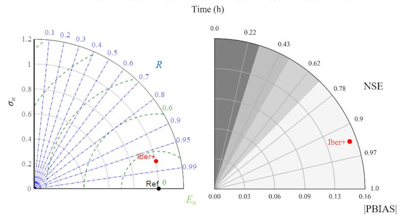
Water 2020, 12, 2319                                                                                 7 of 21

the contributions of Sil River) during the period preceding the day under study (24 h and 5 h for the
non-humid and humid seasons, respectively). A scale factor between the observed and forecasted flow
at Ourense is obtained for the previous day. Then, this factor is applied to the hydrological forecast for
the day of interest to take into account the influence of Sil river at this location.

2.2.2. Hydraulic Model: Iber+
      Iber [36] is a numerical tool that solves the 2D depth-averaged shallow water equations using
the finite volume method. Iber+ [35] is a new implementation of the model in C++ and CUDA [55]
to improve the efficiency of the simulations. The new code is able to achieve a two-order of
magnitude speed-up while attaining the same precision by using graphical processing unit (GPU)
computing high performance computing (HPC) techniques. These optimizations bring the possibility
to employ the model in applications with large spatio-temporal domains [56] or time constrained
applications [8,33]. The software package is freely available and can be downloaded from its official
website (https://iberaula.es). It also includes a graphical user interface (GUI) with preprocessing and
post-processing tools.
      In the present study, Iber+ was applied to analyze flood events in the test area of the city of
Ourense. Figure 1c shows the numerical domain at Ourense, where more than 50 land uses were
defined to model the characteristics of the terrain (Figure 1e). Manning’s coefficients were computed
accordingly to Gonzalez-Cao et al. [57]. The inlet condition was defined by means of the input
hydrograph (critical–subcritical), and the outlet condition was defined using a supercritical–critical
outflow. Turbulence was not taken into account as suggested by [58] and in accordance with similar
works [59–61]. The digital elevation model (DEM) that describes the topography of the area of study
has a resolution of 5 m. The DEM data files were obtained from the Instituto Geográfico Nacional
website (https://www.ign.es/web/ign/portal). The computational domain was discretized using a mesh
with 91,216 unstructured triangular elements, with an average area of 5 m2 .

2.2.3. Automatic Early Warning System
     The early warning system is governed by a set of Python scripts. Basically, the system is triggered
automatically once the precipitation forecasts are published by the local meteorological agency
MeteoGalicia (https://www.meteogalicia.gal). MeteoGalicia provides precipitation information with a
72 h forecast window under a temporal and spatial resolution of 1 h and 4 km, respectively, providing
an adequately representation of rainy situations for the area under scope [33]. Then, the hydrological
simulation is run with the HEC-HMS model, followed by the hydraulic simulations of Iber+ for each
area of interest. The computational step and the results of HEC-HMS are on an hourly scale according
to the precipitation data. The Iber+ model results are also on hourly scale, while the computational
step is adaptive, using a Courant–Friedrichs–Lewy condition [62] value of 0.45. A 24-h forecast horizon
is considered. If any hazard is detected, an alert is issued to the corresponding decision makers.
The general architecture of the system is shown in Figure 2.
     The data necessary to perform the simulations is automatically retrieved by the system. This is
the precipitation forecast and rain gauge data for the basins analyzed (from MeteoGalicia) and the
current river flow (from CHMS) to determine the initial baseflow of the reach. The separation of the
baseflow from the total flow is performed with the Eckhardt method [63], which is applied recursively
from an instant where all the flow could be considered as baseflow. It is also important to note that the
existing dams were not considered in the present work. However, this is a reasonable approach since,
under extreme events, dams have low potential of regulation.
     The hydrological simulations are performed with HEC-HMS using an SCS-CN runoff model.
Although it was meant for single event simulations, the proposed method was designed to overcome its
limitations. For this, the simulation of each sub-basin is separated from the simulation of the river reach.
Each sub-basin is simulated for several fixed precipitation events of 24 h (See Figure 3). Each simulated
event will have an independent curve number based on the precedent conditions as described above.
Water 2020, 12, 2319                                                                                          8 of 21

Additionally, if the simulated event is under the CNmoist class, precipitation of the previous 6 h before
the event is also analyzed, and if precipitation exceeds a threshold (8 mm), the CN will be increased to
97 in order to not interrupt the rain-runoff process. The number of forecasted events depends on the
period that will be predicted and will take data from the precipitation forecast. The number of hindcast
events depend on the characteristics of the basin, for the case of study we found that events prior to
five days before the forecast do not have a significant influence on the flow. In the present analysis,
the precipitation corresponding to the previous days was estimated from rain gauges, although the
system can also run with forecasted precipitation. The second approach is especially useful for poorly
sampled areas or in case of malfunction in the rain gauges. The simulations run with precipitation data
of a single event (24 h), but the simulation period finishes at the end of the prediction period. Then,
the outflow series of the sub-basin is reconstructed with data from each simulation. Starting from the
flow series of the forecast simulations, we sum the run-off coming from the previous events and the
increments in the baseflow. The resulting flow series represent the flow caused by the forecast events
and also the previous ones. The outflow of each sub-basin is then used as input data for the simulation
Water 2020, 12, x FOR PEER REVIEW                                                                            8 of 21
of the river reach. Although this method makes the simulation process more complex, the number of
parameters
are on an hourlyneeded   is the
                     scale       same as
                            according   tofor
                                           thethe  regular SCS-CN
                                                precipitation        method,
                                                              data. The Iber+ making    it especially
                                                                               model results    are alsosuitable
                                                                                                         on hourlyfor
those  cases   were  the data   needed  to parametrize   other  methods is not  available. The
scale, while the computational step is adaptive, using a Courant–Friedrichs–Lewy condition [62]  proposed   method
can beof
value   applied
          0.45. Ato24‐h
                      simulate   longer
                          forecast      periods
                                    horizon       of time than
                                             is considered.  If SCS-CN  without
                                                                any hazard        losing infiltration
                                                                            is detected,               capacity
                                                                                          an alert is issued  to and
                                                                                                                 the
adjusting    the  best CN   for each event   of that period.
corresponding decision makers. The general architecture of the system is shown in Figure 2.

            Figure
            Figure 2.
                   2. Flowchart
                      Flowchart of
                                of the
                                   the Miño
                                       Miño River
                                            River Flood
                                                  Flood Alert
                                                        Alert System
                                                              System (MIDAS)
                                                                     (MIDAS) early
                                                                             early warning
                                                                                   warning system.
                                                                                           system.

     The data necessary to perform the simulations is automatically retrieved by the system. This is
the precipitation forecast and rain gauge data for the basins analyzed (from MeteoGalicia) and the
current river flow (from CHMS) to determine the initial baseflow of the reach. The separation of the
baseflow from the total flow is performed with the Eckhardt method [63], which is applied
recursively from an instant where all the flow could be considered as baseflow. It is also important
to note that the existing dams were not considered in the present work. However, this is a reasonable
approach since, under extreme events, dams have low potential of regulation.
     The hydrological simulations are performed with HEC‐HMS using an SCS‐CN runoff model.
Although it was meant for single event simulations, the proposed method was designed to overcome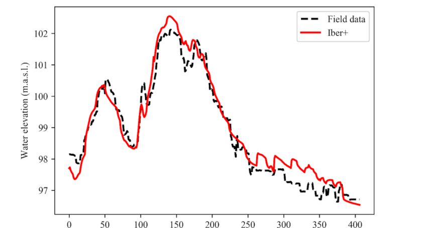
basin is then used as input data for the simulation of the river reach. Although this method makes
the simulation process more complex, the number of parameters needed is the same as for the regular
SCS‐CN method, making it especially suitable for those cases were the data needed to parametrize
other methods is not available. The proposed method can be applied to simulate longer periods of
time than12,
Water 2020, SCS‐CN
2319 without losing infiltration capacity and adjusting the best CN for each event
9 of of
21
that period.
Figure
Figure 3. Procedure
Procedure for
for the
the reconstruction
reconstruction of the sub‐basin
sub-basin outflow series.
After the hydrological simulation, the hydraulic simulations with Iber+ are triggered
Iber+ are triggered for each
zone of interest. Simulations
Simulations can
can be
be launched
launched on
on every
every EWS
EWS execution
execution or
or only
only when
when aa certain safety
safety
threshold is exceeded in the input flow. This second approach can be especially suitable when the
threshold
computation resources
computation resources are limited. Each
Each of the simulations performed with Iber+
Iber+ are
are executed
executed in a
GPU Nvidia
Nvidia RTX 2080ti and require a computational
computational time
time in
in the
the order
order of
of 3–5
3–5 min
min for
for each
each 24 h of
simulated time
simulated time for meshes
meshes of the order of 70–200 k elements. If the modelled reach contains a high
simulations, these
number of zones that require hydraulic simulations, these could
could be
be launched
launched inin parallel
parallel in
in different
different
GPUs to maintain execution times in reasonable values. These These simulations
simulations produce water depth and
hazard maps for maximum values and hourly values. When When some hazard
hazard is detected
detected in the
the hydraulic
hydraulic
simulations, an alert is issued to the corresponding decision makers.
2.3. Statistical
2.3. Statistical Parameters
Parameters to
to Analyze
Analyze the
the Performance
Performance of
of the
the EWS
EWS
Some of
Some ofthe
themost used
most statistical
used parameters
statistical to evaluate
parameters the performance
to evaluate of this type
the performance of procedure
of this type of
procedure were considered to analyze the accuracy of the EWS. In this sense, Spearman correlation
were considered to analyze the accuracy of the EWS. In this sense, Spearman coefficient of coefficient
(r),correlation
of the ratio of
(r),the
theroot mean
ratio square
of the error square
root mean to the standard deviation
error to the standardof deviation
the observed data
of the (RSR),
observed
Nash–Sutcliffe efficiency coefficient (NSE), percent bias (PBIAS), and Taylor diagrams
data (RSR), Nash–Sutcliffe efficiency coefficient (NSE), percent bias (PBIAS), and Taylor diagrams (in(in terms of
the normalized standard deviation (σn ), normalized centered root-mean-square difference (En ) and
correlation (R)) [64], were evaluated following the equations presented below.
r
PN f or 2
i=1 Qobs
i
− Qi
RSR = r 2 (8)
PN
i=1 Qobs
i
− QobsWater 2020, 12, 2319 10 of 21
2
obs − Q f or
PN
i=1 Q i i
NSE = 1 − 2 (9)
PN obs obs
i=1 Q i
− Q
PN f or
i=1Qobs
i
− Qi
PBIAS = PN obs × 100 (10)
i = 1 Qi
s
PN 2
f or
i=1 Qi −Q f or
N
σn = (11)
σobs
s
PN 2
f or
i=1 Qi −Qobs − Qobs
i
−Qobs
N
En = (12)
σobs
PN f or f or obs obs
i=1 Qi − Q Qi − Q
R= (13)
N σ f or σobs
where Qobs is the observed value, Qfor is the forecasted value, N is the total number of observed values,
barred variables refer to mean values, the subscript n refers to the normalized parameter, subscript i
refers to the different samples, and σ is the standard deviation.
3. Results and Discussion
3.1. Hydrologic Module Validation
The accuracy of the hydrological module of the proposed EWS was evaluated by means of
statistical analysis respect to measured river discharge data at Lugo and Ourense stations.
When considering the flow data for the studied period in a daily scale, the results show that the
model is able to predict with a good degree of accuracy the annual cycle of river flow. The model also
shows a clear contrast between dry and humid seasons and is able to reflect the high flow conditions
(Figure 4). This is corroborated when the statistical parameters are analyzed (Table 3). It is considered
a “very good” performance of a hydrological model when the NSE value surpasses 0.7 and the
absolute value of PBIAS is lower than 25% [65–67], these parameters are widely fulfilled in the present
case (NSE > 0.85 and |PBIAS| < 10%) (Table 3). Moreover, the high correlation detected (r > 0.90)
along with the low RSR values obtained (RSR < 0.40) also indicate a good performance according to
Moriasi et al. [65], showing the robustness of the methodology developed.
Table 3. Statistical analysis of the performance of forecasted river flow respect to measured data during
the period 2012–2019.
Statistical Parameter Lugo Station Ourense Station
r 0.97 0.90
RSR 0.30 0.37
NSE 0.91 0.86
PBIAS −5.25 −9.89
In addition, the most important flood events, whose prediction supposes the critical and main
objective from the point of view of EWS, were also evaluated at hourly scale. In particular, those events
where river flow surpassed the 99th percentile for the period under study, were taken into account.
Analyzing the statistical parameters, model results show an accurate prediction of the real river flow
under extreme conditions (Table 4). NSE (>0.7) and |PBIAS| (Water 2020, 12, 2319 11 of 21 of the model developed, which is corroborated by the high correlation values (r > 0.85) along with the low RSR values obtained (0.7) and |PBIAS| ( 0.85) along with the low RSR values obtained (
Statistical Parameter Lugo Station Ourense Station
r 0.89 0.85
RSR 0.42 0.54
Water 2020, 12, 2319
NSE 0.82 0.71 12 of 21
PBIAS −4.08 −6.70
Figure 5.
Figure 5. Forecasted
Forecasted (grey
(grey line) and measured
line) and measured (dotted
(dotted black
black line) river flow
line) river flow for
for the
the most
most dangerous
dangerous
events occurred at (a) Lugo (2016) and (b) Ourense (2019) locations.
events occurred at (a) Lugo (2016) and (b) Ourense (2019) locations.
It is important to remark that PBIAS values obtained in Tables 3 and 4 indicate a slight
overestimation of predicted river flows. However, However, this this type
type ofof systems
systems should
should be conservative,
conservative,
because the consequences of under‐estimate
under-estimate flood events may cause severe damage [8]. In addition, addition,
statistical values show a better performance at the Lugo than at the Ourense location, both in the total
lengthand
series length andininthetheparticular
particular case
case of of
thethe extreme
extreme events.
events. ThisThis is partly
is partly due toduethetofact
thethat
factthe
that the
Miño
Miño at
River River
Lugo at isLugo
underis natural
under natural flow conditions,
flow conditions, whereaswhereas several
several dams damsthe
control control
flow the flow at
at Ourense,
Ourense,
along withalong
the factwith thethe
that fact
Silthat
Tiverthe Sil Tiver
influence at influence
Ourense is atnot
Ourense
directly is simulated
not directly butsimulated
extrapolated but
extrapolated
from Miño datafrom as Miño data above.
described as described above.
When the the obtained
obtained results
resultsare arecompared
comparedwith withother systems
other systems developed
developed in nearby
in nearby areas, the
areas,
hydrological
the hydrologicalmodule shows
module its potential
shows as river
its potential flow flow
as river predictor. Fraga Fraga
predictor. et al. [8] also
et al. [8]use theuse
also HEC‐the
HMS hydrological
HEC-HMS model,
hydrological but under
model, a continuous
but under a continuous simulation
simulationmodemodein nearby
in nearby areas.
areas.This model
This model is
divided into the following two stages: hindcast and forecast. During the
is divided into the following two stages: hindcast and forecast. During the first stage (hindcast), first stage (hindcast), the
hydrological
the hydrological model assimilates
model assimilatesseveral measured
several measured datadata
of 30ofprevious
30 previousdaysdaysin order to reproduce
in order to reproduce the
initial
the soilsoil
initial moisture
moisturecontent
content at the beginning
at the beginning ofof
thethesecond
secondstage
stage(forecast)
(forecast)by bytuning
tuning the
the parameters
parameters
associated to the infiltration of the terrain. In In the
the forecast
forecast stage
stage the
the river
river hydrograph
hydrograph is is computed.
computed.
Althoughititis is
Although important
important to note
to note FragaFraga etfocused
et al. [8] al. [8] onfocused on small
small Galician Galician catchments,
catchments, where
where hydrological
hydrological
forecast is moreforecast is more
sensitive sensitive to precipitation
to precipitation distribution,
distribution, improved improved
values of r andvalues
PBIAS of are
r and PBIAS
obtained
arethe
in obtained
presentin the present
work, work, which
which reinforces reinforces of
the robustness thethe
robustness
methodology of the methodology
proposed. Vieiraproposed.
et al. [68]
Vieira et al.
presented [68] presented
a flood forecast systema flood forecast for
developed system developed of
two sub-basins forAvetwoRiver
sub‐basins
catchment of Ave River
(northern
Portugal) based on the Delft FEWS platform. In this case the meteorological data are obtained from an
ensemble of precipitation predictions. The implementation of the hydrologic and hydraulic models
was carried out using SOBEK software. The calibration of the model parameters was developed
starting from values obtained in the literature and soil characteristics and using the RRL toolkit.
Statistical values are only shown for historical validation period and daily time scale. The EWS
developed in the present work achieves statistical values remarking a higher accuracy even consideringWater 2020, 12, 2319 13 of 21
forecast simulations. A grid-based distributed rainfall-runoff model (GFWS) was implemented in
the Guadalhorce basin (southern Spain) [69], which is a poorly gauged basin, in contrast to the basin
analyzed in our work. The parameters of the model obtained for a small area of the catchment are
transferred to the entire catchment of the Guadalhorce River. In this work, flood warnings obtained
with the GFWS model were compared with those obtained with the low resolution EFAS model.
Higher values of Nash efficiency for forecasted flood events were also obtained in the present work,
showing the good performance of MIDAS.
Therefore, it can be concluded that the hydrological module of the system presented in this work
is able to forecast with high accuracy both the annual cycle (continuous) river flow and the extreme
flood events. The little discrepancies observed between forecasted numerical and measured river flow
can be due to the limitations of these systems—mainly, the simplification of the modelled system and
the uncertainty of the forecast precipitation data. In this sense, the hydrological model supposes an
approximate representation of the reality; therefore, some discrepancies will be expected. Moreover,
although precipitation forecasts provided by MeteoGalicia predict rainy events accurately as shown
in González-Cao et al. [33], the precipitation forecast is, by itself, a source of uncertainty, especially
under situations of extreme rainfall events [33]. Additionally, rain representation provided by rain
gauges can suppose another source of uncertainty. Rain gauges can provide a biased view of the area
under scope since they do not cover the subareas of the basins uniformly. Even with these limitations,
the system proposed provides a great accuracy to predict river flow, especially under extreme flood
events, which impacts the performance MIDAS.
3.2. Hydraulic Module Validation
Once the predicted water flow was shown to reproduce the actual flows with a high accuracy,
the performance of the hydraulic model was also analyzed. For that, the extent and the water elevation
of the flood event registered on December 2019 (from 15 to 31) were computed using Iber+ [17]. On the
one hand, four control areas were defined at study area (green rectangles A, B, C, and D in Figure 1c)
to analyze the accuracy of the numerical results of the flood extension. The control area A corresponds
with a public sport facility (swimming pool) and its recreational zone, the control area B is located near
the gauge station N010 of the CHMS, control area C corresponds with a public path near a national
road, and control area D corresponds to a public thermal baths area. All these control areas are located
near the riverbank and are usually frequented by pedestrians, therefore being of special interest to
issue an alert. On the other hand, the water elevation registered at the gauge station located in control
area B was used to compute the accuracy of the numerical water elevation obtained with Iber+ by
means of Taylor and NSE vs. |PBIAS| diagrams.
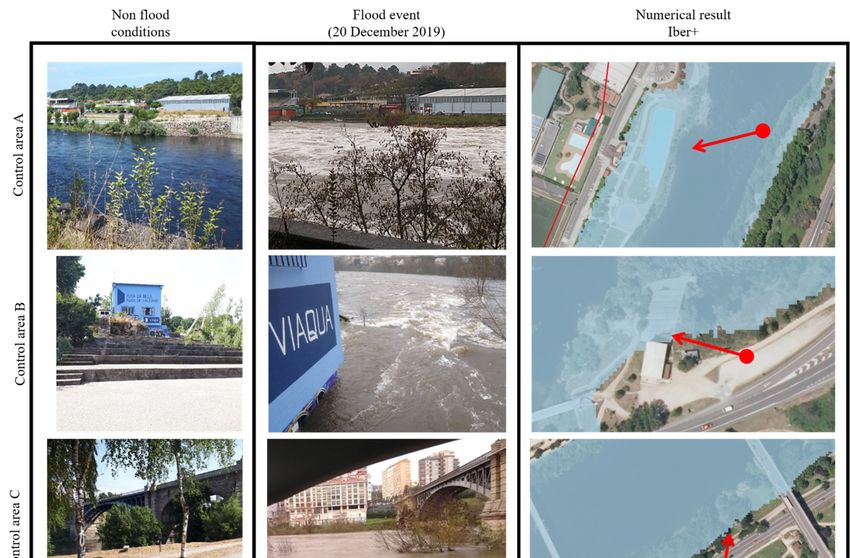
Figure 6 shows the extent of the flood obtained in the numerical simulations along with photographs
taken at the control areas during the flood event within the interval 16:00–16:30 UTC (for all times
throughout the paper) on 20 December 2019. Images corresponding to non-flood conditions are also
depicted, corresponding to a flow within the interval 262–267 m3 s−1 (data obtained from CHMS).
The comparison between photographs taken during the flood and non-flood conditions reveals the
magnitude of the flood event. Visually, the numerical results are quite similar to the field data.
The image of the flood event at the control area A shows that the swimming pool is fully covered by the
flood. The numerical result shows the same situation: the water covers the facility and reaches the wall
near the road. The image at the control area B shows that the flood reaches the building of the gauge
station. The results obtained with Iber+ shows an equivalent situation. Also, the numerical results
show that the flood almost reaches the road. The image corresponding to the control area C shows the
same situation as the numerical results: the flood extension covers the public path and almost reaches
the road. Finally, the thermal baths are fully covered by the flood, and the water almost reaches the
path behind them, as can be observed in the photograph at the control area D. The numerical results
are equivalent to the image of real event.Water 2020, 12, x FOR PEER REVIEW 14 of 21
almost reaches the road. Finally, the thermal baths are fully covered by the flood, and the water
almost reaches the path behind them, as can be observed in the photograph at the control area D.
Water 2020, 12, 2319
The
14 of 21
numerical results are equivalent to the image of real event.
Figure
Figure 6.6.Results
Resultsofofflood
floodextent
extent forfor
each control
each area.
control FirstFirst
area. column depicts
column non‐flood
depicts conditions
non-flood (Q =
conditions
(Q = 265 m s that corresponds to 66th percentile) at the control areas. The second column shows the
265 m 3 s−1 that
3 −1corresponds to 66th percentile) at the control areas. The second column shows the
images
images (photographs
(photographs taken
taken by
by one
one of
of the
the authors)
authors) of
ofthe
theflood
floodevent
event(20
(20December
December2019,
2019,16:00
16:00to
to16:30)
16:30)
and
and the
the third
third column
column shows
shows the
the numerical
numerical results
results obtained with Iber+.
obtained with Iber+. Red
Redarrows
arrowsin
inthe
thethird
thirdcolumn
column
represent the direction of the photograph taken during the
represent the direction of the photograph taken during the flood event. flood event.
The resultsofofthe
The results the
timetime series
series of water
of water elevation
elevation registered
registered from 15from 15 December
December 2019 to 312019 to 31
December
December
2019 at gauge2019station
at gauge N010 station N010 areindepicted
are depicted Figure 7.in This
Figure 7. This
figure showsfigure
theshows the time
time series of the series of
water
the water registered
elevation elevation at registered
the gaugeatstation
the gauge station
(control area(control
B, Figurearea B, Figure
1) and 1) and time
the numerical the numerical
series obtainedtime
series obtained
with Iber+. withnumerical
Visually, Iber+. Visually, numerical
results are similar toresults are similar
field data, to field
which shows thedata, whichofshows
capability the
the model
capability
to forecast of the elevation
water model toaccordingly
forecast water
with elevation accordingly
the river discharge with(Figure
forecast the river
5b). discharge
The Taylorforecast
and the
(Figure |PBIAS|
NSE vs.5b). The Taylor
diagrams andare
the NSE
also vs. |PBIAS|
depicted. Taylordiagrams
diagram are alsothat
shows depicted. of σdiagram
Taylor
the values n , E n , andshows
R are
1.00, 0.22, and 0.97, respectively. The values of NSE and |PBIAS| depicted in the NSE vs. PBIAS diagram
that the values of σ n , E n, and R are 1.00, 0.22, and 0.97, respectively. The values of NSE and |PBIAS|
depicted in the
are 0.94 and NSE vs.
0.15%. The PBIAS
circlediagram
marker are 0.94diagram
in this and 0.15%. The circle
denotes markervalue
a negative in thisofdiagram
PBIAS. denotes
Shaded
aareas
negative
of thevalue
diagramof PBIAS.
refer toShaded areas level
the accuracy of theof diagram
the resultsrefer to the to
according accuracy level of Yilmaz
the criterion the results
and
according
Onoz [67]. to the case,
In this criterion of Yilmaz
the results are inand Onoz corresponding
the range [67]. In this case, the good”
to “very resultsimproving
are in thetorange some
corresponding
extent the results to obtained
“very good” improving
by Fraga toinsome
et al. [8] nearbyextent
smallthecatchments.
results obtained by Fraga
In summary, both et diagrams
al. [8] in
show high agreement between numerical and registered values of water elevation. This indicates that
the system can reproduce this kind of events with high accuracy and can be used to issue an alert.Water 2020, 12, x FOR PEER REVIEW 15 of 21
nearby small catchments. In summary, both diagrams show high agreement between numerical and
registered
Water 2020, 12, values
2319 of water elevation. This indicates that the system can reproduce this kind of15events
of 21
with high accuracy and can be used to issue an alert.
Figure7.7.Upper
Figure Upperpanel:
panel:time
time series
series of of water
water elevation
elevation obtained
obtained at gauge
at gauge station
station (black(black
dasheddashed line)
line) and
and using
using Iber+Iber+ (red at
(red line) line) at gauge
gauge station
station N010N010 (control
(control area
area B). B). Lower
Lower left panel:
left panel: Taylor Taylor diagram
diagram of theof
the series
time time series of water
of water elevation
elevation obtained
obtained with using
with Iber+ Iber+ the
using thedata
field fieldasdata as reference.
reference. Lower
Lower right right
panel:
NSE vs. |PBIAS| diagram of the numerical water elevation using the field data as reference. Marker
panel: NSE vs. |PBIAS| diagram of the numerical water elevation using the field data as reference.
Markernegatives
denotes denotes negatives
values of values
PBIAS ofandPBIAS andareas
shaded shaded areas
refer refer
to the to the of
criterion criterion
[44] to of [44] to
define thedefine the
level of
level of accuracy:
accuracy: very good,very good,
good, good, satisfactory,
satisfactory, and unsatisfactory
and unsatisfactory (from lighter(fromto lighter
darker).to darker).
3.3.
3.3.Analysis
Analysisand
andPredictability
PredictabilityofofRiver
RiverFlood
FloodRisk
RiskSituations
Situations
The
Thevalidation
validationofofthe thehydrologic
hydrologicand andhydraulic
hydraulicmodules
moduleshas hasshown
shownaagoodgoodforecast
forecastofofriver
riverflow
flow
under flood events as well as a good representation of the areas affected by these flood
under flood events as well as a good representation of the areas affected by these flood events. The events. The final
step
finalis step
to focus
is tothe system
focus on critical
the system on areas from
critical thefrom
areas pointthe
of view
pointofofcritical
view ofinfrastructures damage.
critical infrastructures
The ultimate goal is that the system can report dangerous situations well in advance
damage. The ultimate goal is that the system can report dangerous situations well in advance so that so that decision
makers
decision can take appropriate
makers mitigation mitigation
can take appropriate measures. In this sense,
measures. In the
thishazard
sense, in
thethe city ofinOurense
hazard the cityisof
analyzed. The criterion employed to define a hazard area was the presented
Ourense is analyzed. The criterion employed to define a hazard area was the presented by Cox by Cox et al. [70]. Firstetof
al.
all, after am in-depth study of the hazardous areas affected by different water flows,
[70]. First of all, after am in‐depth study of the hazardous areas affected by different water flows, the alert statusthe
was
alertdivided
status in four
was levels (see
divided Tablelevels
in four 5 for (see
specific thresholds).
Table The first
5 for specific of them, pre-activation,
thresholds). The first of them, defines
pre‐
the average conditions of the river reach. In the second level, activation, some risk
activation, defines the average conditions of the river reach. In the second level, activation, some can occur in areas
risk
accessible
can occurtoinbut notaccessible
areas frequented toby
butpedestrians.
not frequented The third state is pre-alert
by pedestrians. where
The third hazard
state can occur
is pre‐alert wherein
areas frequented by pedestrians. The last one is the alert state where the flood causes
hazard can occur in areas frequented by pedestrians. The last one is the alert state where the flood hazard in areas
frequented
causes hazard by pedestrians and severe
in areas frequented bydamage to infrastructures.
pedestrians and severe damage to infrastructures.Water 2020, 12, 2319 16 of 21
Table 5. Hazard thresholds for the Minho River at Ourense City.
Alert Status Min Flow (m3 /s) Max Flow (m3 /s)
Pre-activation 0 511
Activation 511 1253
Pre-alert 1253 2000
Alert 2000 -
Once the thresholds that define the different risk situations were evaluated, an analysis of the
observed and predicted flow was carried out in order to assess the EWS’s ability to accurately issue an
alert. In this sense, 17 alerts should have been issued based on the flow observed during the eight
years of the simulated period (Table 6). The EWS accurately predicted 13 of them, 4 were missed and
5 were false positives. This means that the proposed system is able to predict the 76% of the alerts and
28% of the alerts issued are false positives, which shows a good performance of the designed system in
terms of predictability of risk situations.
The system is able to issue an alert based on the hydrological forecast and also to provide detailed
water depth, water velocity, and hazard maps in terms of hydraulic model simulations. Both the
maximum values and hourly evolution of these parameters are obtained for the forecasted period.
Figure 8 shows the average number of days under hazard conditions per year. It can be observed that
many zones frequented during outdoor activities can be affected by hazard conditions for more than
10 days per year on average, emphasizing the requirement of an accurate EWS. Figure 9 shows the
maximum extension of the hazardous area for each of the warning levels defined in Table 5. This map
shows that the differences between two warning levels are minimal in certain areas, illustrating the
necessity of accompanying the alert reports with detailed flood maps. This information provides a
detailed view of areas affected under the respective flood event. In this way, decision makers can
have2020,
Water enough dataPEER
12, x FOR to evaluate
REVIEW the situation correctly and take more precise and effective measures,
17 of 21
diminishing the damage provoking by floods.
Figure 8. Average days under risk per year.
Figure 8. Average days under risk per year.Water 2020, 12, 2319 17 of 21
Table 6. Contingency table with the number of alert events observed and forecasted. From a total of 2922 events
analyzed, 13 were correct positives, five false-positives, four missed alerts, and 2900 correct negatives.
Observed
Total
Alert Non-Alert
Alert 13 5 18
Forecasted Figure 8. Average days under risk per year.
Non-Alert 4 2900 2904
Total 17 2905 2922
Figure 9.
Figure Maximumextents
9. Maximum extentsof
of the
the hazardous
hazardous area
area under
under the
the different
different alert
alert stages.
stages.
4. Conclusions
4. Conclusions
This paper presents MIDAS, a new flood early warning system based on integrated hydrologic
This paper presents MIDAS, a new flood early warning system based on integrated hydrologic
and hydraulic models. The automatic operation of MIDAS is governed by a set of Python scripts.
and hydraulic models. The automatic operation of MIDAS is governed by a set of Python scripts.
Starting from precipitation forecast, the rainfall-runoff process is simulated with the HEC-HMS model
Starting from precipitation forecast, the rainfall‐runoff process is simulated with the HEC‐HMS
to obtain the predicted river flow, which is used to run Iber+ for each area of interest. An alert is issued
model to obtain the predicted river flow, which is used to run Iber+ for each area of interest. An alert
when a hazardous situation is detected.
is issued when a hazardous situation is detected.
The results show the high capability of the system to accurately forecast river flows and are
The results show the high capability of the system to accurately forecast river flows and are
representative of the flooded areas under extreme events. In fact, MIDAS was able to predict 13 of the
representative of the flooded areas under extreme events. In fact, MIDAS was able to predict 13 of
17 alerts that took place over the study period, which is a good performance in terms of predictability of
the 17 alerts that took place over the study period, which is a good performance in terms of
risk situations. This good performance of the system, together with the capability to provide detailed
predictability of risk situations. This good performance of the system, together with the capability to
hazard maps, can provide information to decision makers to evaluate flood situations and to take
provide detailed hazard maps, can provide information to decision makers to evaluate flood
precise and effective measures that mitigate the damage associated with these events.
situations and to take precise and effective measures that mitigate the damage associated with these
Finally, it is important to remark that, despite MIDAS being applied to the Miño River,
events.
its implementation in other basins is straightforward. This approach is especially valuable for
areas with low sampling resources, showing its potential in future applications.
Author Contributions: D.F.-N., O.G.-F., J.G.-C., and M.G.-G. conceived the study; D.F.-N., O.G.-F., and J.G.-C.
conducted the research and developed the software; M.G.-G. supervised the research development; D.F.-N.,
O.G.-F., J.G.-C., C.d.G., J.A.R.-S., C.R.d.P., and M.G.-G. analyzed the results; D.F.-N., O.G.-F., J.G.-C., and M.G.-G.
wrote the manuscript; C.d.G., J.A.R.-S., and C.R.d.P supervised the research, provided field data, and revised the
manuscript. All authors have read and agreed to the published version of the manuscript.
Funding: This research was partially supported by INTERREG-POCTEP under project RISC_ML (Code:
0034_RISC_ML_6_E) co-funded by the European Regional Development Fund (ERDF) and by Xunta de Galicia
under Project ED431C 2017/64-GRC “Programa de Consolidación e Estruturación de Unidades de Investigación
Competitivas (Grupos de Referencia Competitiva).” O.G.F. is supported by Xunta de Galicia grant ED481A-2017/314.
Acknowledgments: The aerial pictures used in this work are courtesy of the Spanish Instituto Geográfico Nacional
(IGN) and part of the Plan Nacional de Ortofotografía Aérea (PNOA) program.You can also read