Interaction of Estuarine Morphology and adjacent Coastal Water Tidal Dynamics (ALADYN-C)
←
→
Page content transcription
If your browser does not render page correctly, please read the page content below
Die Küste, 89, 2021                                                     https://doi.org/10.18171/1.089108

Interaction of Estuarine Morphology and adjacent
Coastal Water Tidal Dynamics (ALADYN-C)
Krischan Hubert1, Andreas Wurpts2 and Cordula Berkenbrink2
1 Nds. Landesbetrieb für Wasserwirtschaft, Küsten- und Naturschutz,
  krischan.hubert@nlwkn.niedersachsen.de
2 Nds. Landesbetrieb für Wasserwirtschaft, Küsten- und Naturschutz

Summary
Long term tidal dynamic changes comprise a share of multiple possible influencing pro-
cesses. In the shallow Wadden Sea in the south eastern German Bight, morphological
changes – both natural and those manmade – are key contributors, as coastal relief and
tidal wave are shaping and interacting with each other. Several publications have analysed,
how bathymetrical changes in the estuarine zone due to river construction measures influ-
ence the tidal regime inside the investigated entity. This study aims at identifying, how far
those tidal dynamic changes will have an impact on adjacent coastal waters and give an
estimate how they are reflected in the data of surrounding tide gauges. The investigation is
based on comparisons of tidal characteristics for different morphological conditions of
selected regions along the German coastline by means of numerical modelling. A cross-
scale model domain was set up to simulate the hydrodynamics of the entire Greater North
Sea with a special focus on the highly resolved German tidal waters. Digitized historical
conditions for the Ems and Weser estuary prior to major human activities along the rivers
were used to reproduce the tidal regime of the corresponding time period within the large-
scale environment of the overall domain. Morphological changes that account for single
measures, such as the land subsidence due to gas extraction, were analysed isolated from
other changes. The differences of the simulation results are compared to values from con-
trol runs with the present bathymetrical state. This illustrates the region of influence, in
which tides are effected from locally limited bathymetrical changes.

Keywords
tidal dynamics, sea level rise, long-term trend, estuary, Ems, Weser, North Sea, historic
bathymetry, coastal morphology, cross-scale modelling, land subsidence due to gas extrac-
tion, ALADYN, SCHISM

Zusammenfassung
Langzeitänderungen der Tidedynamik setzen sich aus einer Vielzahl von möglichen ursächlichen Prozessen
zusammen. Im flachen Wattenmeer haben morphologische Veränderungen – sowohl natürlicher als auch
anthropogen geprägter Art – einen entscheidenden Einfluss, da sich Tidewelle und Küstenrelief gegenseitig
stark beeinflussen und formen. Mehrere wissenschaftliche Arbeiten haben bereits untersucht, inwiefern
Änderungen der Bathymetrie von Ästuaren im Zuge von Flussausbauten das Tideregime innerhalb des
Die Küste, 89, 2021                                                     https://doi.org/10.18171/1.089108

betrachteten Gebiets beeinflussen. Dieser Beitrag geht der Frage nach, wie weit sich diese Änderungen der
Tidedynamik auch in außerhalb liegenden Gebieten feststellen lassen. Die Untersuchungen basieren auf
Vergleichen von Tidekennwerten, die mittels numerischer Modellierung für verschiedene morphologische Zu-
stände ausgewählter Abschnitte der deutschen Nordseeküste nachgebildet wurden. Für diesen Zweck wurde
ein skalenübergreifendes Strömungsmodell erstellt, welches die Hydrodynamik des gesamten Nordseegebietes
simuliert. Im Fokus der Untersuchungen stehen dabei die im Modellgebiet hochaufgelösten deutschen Tide-
gewässer. Digitalisierte Bathymetrie-Datensätze von historischen Ausbauzuständen der Ems und Weser,
die bis vor die maßgebenden menschlichen Eingriffe in die Flussläufe zurückreichen, wurden verwendet, um
die lokalen Gezeiten der entsprechenden Zeiträume innerhalb des gesamtübergreifenden Modellgebietes ab-
bilden zu können. Veränderungen, die auf Einzelmaßnahmen zurückzuführen sind, wie Bodensenkungen
infolge von Gasentnahme, werden isoliert von anderen Einflussfaktoren analysiert. Die Differenzen der
Simulationsergebnisse aus dem Vergleich mit Werten aktueller Ausbauzustände stellen den Einflussbe-
reich dar, in welchem lokal begrenzte Änderungen der Bathymetrie das Tideregime beeinflussen.

Schlagwörter
Tidedynamik, Meeresspiegelanstieg, Trend, Ästuar, Ems, Weser, Nordsee, historische Bathymetrie,
Küstenmorphologie, skalenübergreifendes HN-Modell, Landsenkung infolge Gasentnahme, ALADYN,
SCHISM

1    Introduction
The motivation for the joint research project ALADYN was to gain a better understanding
of the composition of observed tidal range changes within the German Bight. Therefore,
the three separate parts of the project would each aim on identifying and analysing different
potential factors that may have contributed to the observed trends. One task within
ALADYN was to analyse tidal regime changes induced by local bathymetrical changes. The
goal of this project part was to analyse how far local hydrodynamic changes would spread
into adjacent coastal regions. The focus is on the region around the estuaries Ems and
Weser, both entering the North Sea at the Lower Saxonian coastline.
    The hydrodynamics of the German Bight, its coastal morphology and a vast number of
natural processes as well as human activities are greatly dominated by the influence of the
tides. Along the coastline, there are numerous tide gauges, some of which are already in
operation since up to over 150 years. Figure 1 shows yearly mean tidal high (MHW) and
tidal low water (MLW) levels for selected gauge stations throughout the German Bight
since begin of their operation.
    Trend analysis of long-term tide records indicate a general increase of both MHW and
MLW with rates of several centimetres up to a few decimetres within one century. Whereas
the trends of the high waters are rather similar throughout the different gauge stations,
trends in low waters are slightly diverse, as the low waters might react stronger on local
morphological variations due to greater influence of bottom friction. For example, the low
waters near the estuaries – i. e. Bremerhaven and Emden - seem to decrease due to the
constant deepening of the neighbouring navigational channels. But there is one trend that
is valid for all gauge stations: The MLW is always either falling or rising less strong than
the corresponding MHW. Thus, the rates of mean tidal range (MTR) increase are all posi-
tive (see Table 1).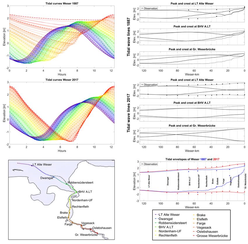
Die Küste, 89, 2021                                                https://doi.org/10.18171/1.089108

Figure 1: Left panel: Overview. Middle and right panel: Yearly mean tidal high and low waters [cm]
with arbitrary offset at different gauge stations throughout the German Bight. The positions are
indicated in the left panel. Data provided by German Federal Waterways and Shipping Admin-
istration (WSV).

The observed trends are composed from a variety of different processes that all contribute
with different magnitudes and signs and that may interact linearly and non-linearly with
each other. In addition to global factors like sea level rise, vertical land movement, varia-
tions in wind climate or astronomical constellations, changes of the tidal regime can also
mirror local effects (Haigh, 2020). Morphology is a key factor on such local scales, especially
in shallow coastal zones. Here the tidal regime is dominated by the bathymetry and corre-
spondingly susceptible to morphological changes (Niemeyer and Kaiser 1999). The Wad-
den Sea represents an inherently morphodynamical system, which is subject to continuous
rearrangement. Contributors are naturally imposed shifts and transformations of the tidal
channels, flats, basins and barrier islands as well as anthropogenically induced changes due
to navigational purposes or demands of coastal protection (Elsebach et al. 2007, Herrling
and Niemeyer 2008).
    In both Weser and Ems estuary, the major human interventions and consecutive mor-
phological reactions started more than 130 years ago. After smaller previous measures the
so-called Franzius corrections started in 1887 and were the beginning of a substantial rear-
rangement of the Outer and Lower Weser riverbeds, in order to obtain the access of the
port of Bremen to the open sea. The corrections comprised a transition from a fairly shal-
low, curvy and branched riverbed to a deeper, comparatively narrow and single-branched
channel (Elsebach et al. 2007, Franzius 1888, Niemeyer, 2000). Several consecutive adap-
tations of the river for increasing navigational demands followed up to present times
(BUND, Portal Tideweser).
    Considering the tidal range, the modifications engendered a drastic amplification of the
tidal wave amplitude along the estuaries. Figure 2 displays the change of tidal range over
time for lower Weser and Ems rivers. Before the Franzius corrections, the tidal wave was
almost completely damped on its way through the estuary while today it is fully reflected
and also steepened with strongly amplified range. At the head of the estuary, the present
tidal range exceeds the one at the mouth, whereas it used to be close to zero before the
corrections.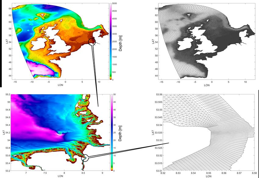
Die Küste, 89, 2021                                                 https://doi.org/10.18171/1.089108

   The evolution of the Ems estuary’s morphology follows a similar pattern (Herrling and
Niemeyer 2007b). Here, modifications also started in the second half of the 19th century,
but continuous tide gauge records do not date back as long as for the Weser.
Table 1: Linear trends [mm/a] of yearly mean tidal high water, low water and tidal range values for
the time of recording at different gauge stations throughout the German Bight. The positions are
indicated in Figure 1. Data provided by WSV.
                                                                        Linear trends [mm/a]
 Tide gauge                                             Period          MHW MLW            MTR
 Husum                                                  1901 – 2016     3.28     0.11      3.17
 List                                                   1937 – 2015     3.36     0.47      2.89
 Wangerooge West                                        1951 – 2017     3.34     1.60      1.74
 Langeoog                                               1951 – 2017     2.38     1.10      1.28
 Norderney Hafen/Riffgat                                1891 – 2017     2.80     1.33      1.47
 Borkum Südstrand /Fischerbalje                         1931 – 2017     3.09     1.18      1.91
 Leuchtturm Roter Sand/Alte Weser                       1936 – 2017     4.49     2.84      1.65
 Helgoland Binnenhafen                                  1910 – 2016     2.16     0.72      1.44
 Wilhelmshaven Alter Vorhafen                           1873 – 2017     2.93     0.65      2.28
 Emden Neue Seeschleuse                                 1901 – 2017     2.33     -0.29     2.62
 Cuxhaven Steubenhöft                                   1843 – 2017     2.25     1.31      0.94
 Bremerhaven Doppelschleuse/Alter Leuchtturm            1881 – 2017     2.74     -1.68     4.42

The anthropogenic interventions caused significant changes of the tidal regime within the
estuaries of Ems and Weser itself. Those effects have already been thoroughly analysed
with hydrodynamic modelling approaches (Elsebach et al. 2007, Herrling and Niemeyer
2008, Herrling et al. 2014).
    This project is expanding the existing scope of the investigations. It is not only dealing
with the tidal regime changes within the estuaries, but also whether how strong and how
far these inner-estuarine changes also affect the adjacent coastal waters and tidal gauges
located there. We examine possible interactions of the estuaries with the coastal zone and
analyse, how far the hydrodynamic changes spread outside of the region of the correspond-
ing morphological changes. This objective is addressed using numerical simulations of the
large-scale tidal dynamics with comparisons between present and historical morphological
conditions. The method allows to analyse single measurements or regions isolated from
surrounding morphological changes. This way, shares of tidal characteristic changes can be
assigned to certain events including the nonlinear behaviour of the hydrodynamics.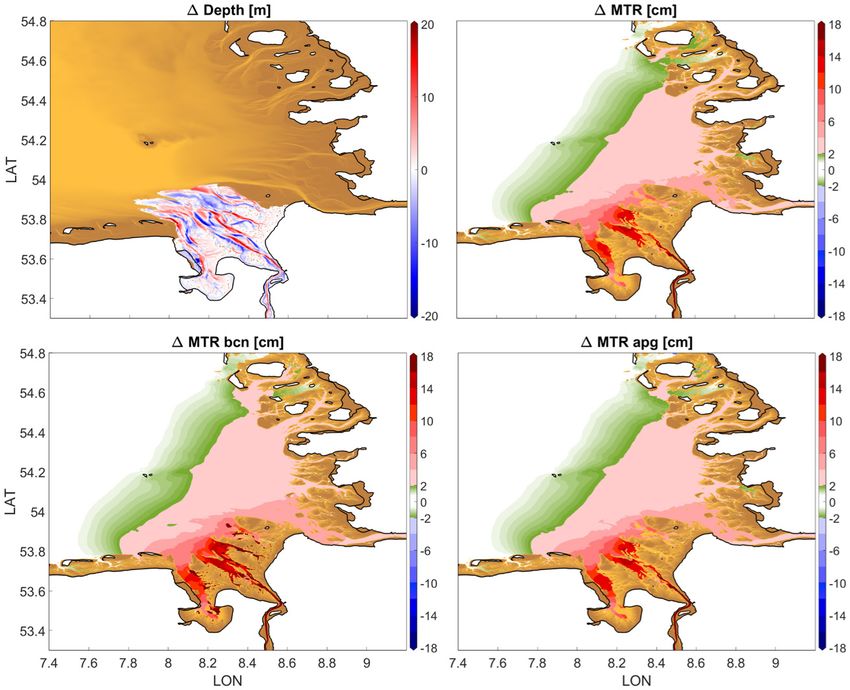
Die Küste, 89, 2021                                                  https://doi.org/10.18171/1.089108

Figure 2: Yearly mean tidal range values [cm] along the Weser (upper panel) and Ems (lower panel)
estuaries from 1880–2018. Red lines indicate a position near the head of the estuary, blue lines near
the mouth and green lines approximately half way in between. Data provided by WSV. (Elsebach
et al. 2007 and Niemeyer 2000 (unpublished)).

2    Methodology
For the purpose of this study a numerical model domain was set up, that not only covers
the investigation area but is well extended above the Greater North Sea into parts of the
North East Atlantic. This approach offers several advantages over models with smaller
extend or nested cascades of models:
    • It bypasses model cascades, as the tidal oscillations at the seaward open boundaries
      can be forced directly through tidal constituent phases and amplitudes in the open
      ocean. Due to the great distance between open boundary and investigation area, the
      velocity boundary condition can be omitted.
    • The propagation of the tidal wave is physically consistent throughout the entire model
      domain. There is a bi-directional interaction between the coastal zone and the open
      sea, which would be missing in a one-way nested application. Influences from model
      boundary forcing are avoided.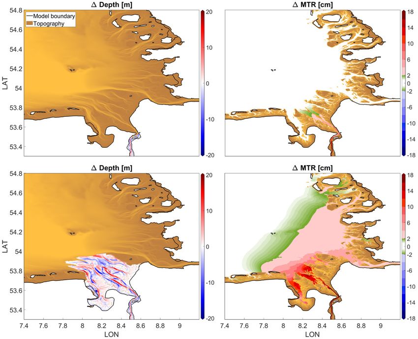
Die Küste, 89, 2021                                                https://doi.org/10.18171/1.089108

    • The investigation area is not limited pre-hand to an inner domain or specific region.
      This is an important factor, as the spatial distribution is part of the analysis and is
      considered as unknown initially.
The procedure of the evaluation of morphologically induced tidal regime changes happens
as follows: For each analysis we perform two simulations on the same numerical grid, which
is beforehand optimized for two morphological states. The first simulation is the control
run. It contains the present state bathymetry and is equal for all analysis. The bathymetry
of the second simulation is replaced by a historical data set in the respective area of interest.
All remaining parts of the model and all boundary conditions remain exactly the same.
After calculating the differences of certain tidal characteristics between the two simulations,
it is possible to derive spatial information on how far these differences exceed the manip-
ulated area.
     Analysis are carried out over a period of at least two spring-neap cycles. For the com-
parisons, synthesized mean tidal curves for elevation and u- and v-velocities are derived
from all single tidal cycles for each computational node in the domain. This procedure
ensures that the calculated differences comprise an average over the diurnal, fortnightly
and monthly inequalities of the tide. It is not only an average of single parameters like peak
and crest heights or maximum flood and ebb velocities. The synthesized tidal curve displays
an averaged tidal curve over 12.4 hours with a temporal discretization of six minutes (see
Section 3).

2.1 Model Setup
The simulations are carried out with the semi-implicit, finite element model suite SCHISM
(Zhang et al. 2016, version 5.6.1) which is tailored to seamless cross-scale applications. The
domain is – in the horizontal plane – discretized with an unstructured grid of triangular and
quadrangular elements.
    Figure 3 gives an overview of the model domain. The western seaward open boundary
spans from the north-western tip of Spain across the Atlantic at ~16° west up to Iceland.
The northern seaward open boundary spans from Iceland across the Norwegian Sea down
to western Norway. The most easterly part of the model is the Kattegat. The model bound-
ary towards the Baltic Sea follows the coast of the Danish major islands Funen and Zealand,
connecting the Danish and Swedish mainland. The connecting belts to the Baltic Sea are
not considered as open boundaries, as we consider the influence it has on the investigation
area in the German Bight as insignificant, especially as it would have to encounter the net-
direction of both the Norwegian and so-called “Silberrinnen” tidal wave (See- und Ozean-
handbücher 1958). In the German Bight, the different entities of the Wadden Sea – tidal
inlets, tidal basins and barrier islands – are resolved. The model includes the estuaries of
the Ems, Weser and Elbe rivers up to their tidal barriers in Herbrum, Bremen and
Geesthacht respectively. Also parts of the tidal Eider River are included in the Model do-
main. Ems, Weser and Elbe River are supplied with discharge open boundaries. The dis-
charge boundaries are located upstream of the tidal barriers which are represented by weir
structures in the model (Ateljevich et al. 2014). Tributaries of Ems and Weser River as well
as the Eider River are treated as sources.
    The SCHISM model enables maximum flexibility for the horizontal discretization. Be-
cause the terms imposing the most stability constraints are handled numerically implicit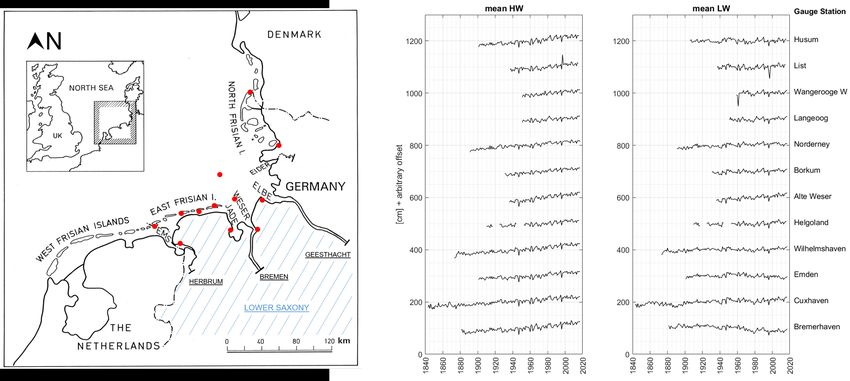
Die Küste, 89, 2021                                                https://doi.org/10.18171/1.089108

and advection of momentum is treated by means of an un-Trim-like Lagrange approach, a
wide range of different mesh sizes is possible, as Courant numbers far beyond 1 are possible
(Zhang et al. 2016). We highly resolve the investigation area around the estuaries and the
Wadden Sea and have a very coarse resolution in the Greater North Sea and Atlantic parts
of the model. This way, around 90 % of the ~675 thousand horizontal computational
nodes and ~ 1.2 million elements are inside the investigation area, which in contrast only
covers less than 1 % of the model domain (compare Table 2). Consequently, the large
overall domain has little effect on the computational time.
Table 2: Numbers of grid nodes, area size and Element size range for different regions of the
model domain. Values are only approximate.
Region                                 number Share of           Area Share of     Element
                                      of nodes        nodes              Area    size range
                                                -          %      km2       %              m
Inner estuaries of Ems Weser Elbe       100000          14.8     1100     0.05      5* – 200
Wadden Sea                              500000          74.1    15000     0.65      50 - 200
Remaining Greater North Sea              50000            7.4 700000     31.15 200 – 10000
Remaining Model domain                   25000            3.7 1530000    68.15 3000 – 50000
Total                                   675000         100.0 2246100    100.00     5 - 50000
*direction of quad. elements perpendicular to flow direction

Figure 3: Overview of the model domain (Hubert et al. 2019). Top left panel shows the spatial
extent, colors indicate the bathymetry. Bottom left panel shows the German Bight as an enlarged
detail of the model. Top right panel shows the unstructured horizontal grid, which’s local resolu-
tion is aligned with respect to the corresponding model depth. Bottom right panel shows an ex-
emplary transition from triangular to quadrangular elements at the head of Lower Weser estuary.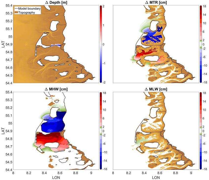
Die Küste, 89, 2021                                               https://doi.org/10.18171/1.089108

The majority of elements are of triangular shape. Their sizes are determined by the sur-
rounding depth (compare Figure 3). In the channels of Ems and Weser as well as in selected
tidal channels, where there occurs distinct bidirectional flow, quadrangular elements are
used to ensure a proper representation of the channels cross-sections and further reduce
numerical diffusion and element numbers. As the Ems river gets comparatively narrow
close to its tidal barrier, element sizes perpendicular to the flow direction go under 10 me-
ters, in order to assure a minimum number of five to six active nodes in the cross-section
during low water conditions. In the vertical discretization, localized sigma coordinates
(LSC2) are used (Zhang et al. 2015).
    Bathymetrical information for the model is compiled from several sources (compare
Table 3). In the larger domain of the Greater North Sea and Atlantic we use open source
data from EasyGSH-DB and EMODnet. Within the Lower Saxony Coastal Zone and es-
tuaries, we use state owned high-resolution LiDAR and sounding data. Bathymetry for the
tidal parts of the Eider River were provided by the Schleswig-Holstein Agency for Coastal
protection, National park and Marine Conservation.
Table 3: Present and historic bathymetries used in the numerical model
Region                                          Period*         Source
                                             Present
Atlantic and parts of the North Sea                  2016          EMODnet
German Bight and parts of the North Sea              2016          EasyGSH-DB
Parts of the tidal Eider River                       2012          State of Schleswig Holstein
Ems estuary                                          2015          State of Lower Saxony
Jade Estuary                                         2012          State of Lower Saxony
Weser estuary                                        2012          State of Lower Saxony
Elbe estuary                                         2010          State of Lower Saxony
East Frisian islands                              2013- 2016       State of Lower Saxony
                                             Historic
                                              1650, 1750, 1860,
Entire Lower Saxony coastline                                      Homeier et al. 2010
                                                     1960
Ems                                                  1937          Herrling and Niemeyer 2007a
Lower Weser                                          1887          Elsebach et al. 2007
Outer Weser                                          1870          Dev. within this project
East Frisian islands                                 1960          Dev. within this project
* data might not be limited to a single year but cover a larger time span

Considering the historical bathymetries, a number of data sets have been developed within
former research work as well as within this research project. They have been developed by
comprehensive digitization of historic navigational charts or other ancient documents. Fig-
ure 4 shows exemplarily the setup of the historic bathymetry of the outer Weser estuary.
    Because bathymetrical information more than a hundred years ago was sparse – both
in space and time – as well as much less accurate compared to today’s possibilities, there
are a few limitations that need to be pointed out:
    • The historical data sets, especially for larger areas, never represent a close instant of
      time. The preparation of navigational charts in 19th and early 20th century took several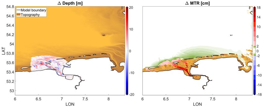
Die Küste, 89, 2021                                                  https://doi.org/10.18171/1.089108

      measuring campaigns to complete and thus are compiled from data that was collected
      over a period of sometimes several years.
    • For larger areas, there are sometimes not enough maps of the same period available
      to cover the whole area, or certain maps have to be omitted due to insufficient quality
      or other reasons. For example, the historical bathymetry for the Ems estuary is com-
      piled from different maps covering several decades (Herrling and Niemeyer 2007a).
    • As ancient maps were mainly created for navigational purposes, information outside
      the navigational channels, i.e. tidal flats, are provided only with little depth infor-
      mation. These gaps have to be filled with assumptions.
    • The vertical reference system differs from today’s vertical reference and thus depths
      need to be adjusted. In some cases, depth will be given with reference to local low
      water marks. Here, adjustment of the depths is a lot more difficult, as it has to be
      done with historical tide gauge data.
Also present bathymetrical data sets face some of these problems, especially when looking
at the larger offshore domain of the North Sea, where on the one hand depth are still
shallow, so that inaccuracies can have a notable impact on the simulated tide but on the
other hand such inaccuracies are unavoidable with respect to the size of the area and the
absence of GNSS kinematic reference.
    Therefore it is very important to straighten out that the derived results in this study
must always be looked at with respect to the range of uncertainties.

Figure 4: Homeier charts (Homeier et al. 2010) of the outer Weser and Jade estuary region for the
state of 1860 showing supra-, inter-and subtidal areas (left panel) and Triangular Irregular Network
(TIN) of the same region for the reconstructed state of 1870. The background shows a historical
navigational chart of 1870 (Lang 1973) that was used to digitize the elevation data for the TIN.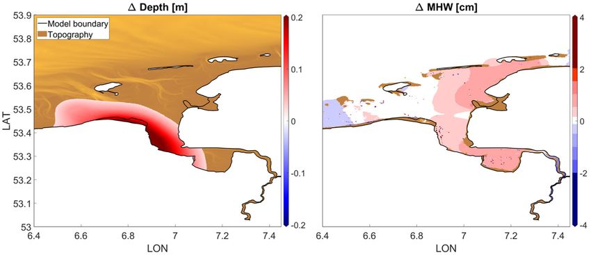
Die Küste, 89, 2021                                               https://doi.org/10.18171/1.089108

2.2 Model Calibration
Due to the model setup and its completely new spatial domain covering a large area, the
calibration process took a big share within the project. The ALE approach of the SCHISM
model requires the calibration to iteratively optimize the model grid, since a specific range
of very high CFL values has to be met. During the evaluation process of the study, neces-
sary modifications of the grid resolution setup also had to be implemented continuously.
The model was calibrated with and validated for different time periods from 2014 to 2017.
    The overall results also strongly depend on the used turbulence closure scheme: The
cross-scale domain shows depth variations between several thousand meters at the conti-
nental shelf and constantly wetting and drying cells next to tidal channels of 10 m depth in
the Wadden Sea and estuaries.
    Shallow water wave equation models, when turbulence is considered in a boussinesq-
approximated way (e.g. two equation turbulence models) basically assume the complete
water depth as the turbulent wall boundary layer.
    Especially without meteorological or wave forcing at the surface, the specific configu-
ration of the turbulence model may pose severe problems finding a realistic compromise
between the open ocean and deeper North Sea areas and the Wadden Sea and estuaries.
This is further complicated with vertical grid resolution issues.
    The following parameters had to be considered in the calibration of the model:
    • Horizontal grid and time stepping
      The most important part was the design of the unstructured mesh in the horizontal
      plane, since the mathematical approach requires strict compliance with the appropri-
      ate CFL range. It has to accommodate optimal resolution of the investigation area in
      combination with a reasonable overall mesh size, time stepping and computational
      time. Several meshes for the same domain were set up and tested. Especially in the
      Wadden Sea and estuarine zone, the setups have developed intensely over time. Be-
      sides the implementation of quadrangular elements in the estuarine zone and stepwise
      refinement of the entire Wadden Sea from Den Helder to Esbjerg, a major step was
      to improve the grid design for Ems and Weser river, so that it can handle both his-
      torical and present states with flow-parallel quadrangular elements, even though po-
      sitions and directions of the main channels differ greatly in some parts between the
      two conditions. Additionally, the model domain includes several areas between his-
      torical and present dyke lines. The current grid is optimized for a time stepping of
      200 seconds.
    • Vertical discretization
      In the vertical plane, different solutions for discretization have been tested from 2D,
      pure z, hybrid sigma/z-coordinates to localized sigma coordinates (Zhang et al. 2015).
      The current setup uses LSC2 with a focus on the top 200 m, i. e. continental shelf.
    • Bottom friction and turbulence closure scheme
      The model was calibrated using different regional friction coefficients. The bottom
      friction is calibrated in alignment with present conditions and adopted for the histor-
      ical states. This of course is a compromise and has the consequence, that results will
      not be satisfactory in all places and morphological states. But since friction is also one
      of the boundary conditions, this procedure ensures that we analyse differences in-
      duced only by bathymetrical changes and not from friction coefficient variations or
Die Küste, 89, 2021 https://doi.org/10.18171/1.089108
other boundary conditions. Bottom roughness is given as roughness length z0 with a
constant value of 2 mm.
• Bathymetry
As bathymetrical data is only accurate up to a certain level, it is valid and probably
necessary to adjust it as a parameter in the calibration process in the range of its
uncertainties (Verboom et al. 1991). Especially the historical bathymetries lack on
accuracy, as stated before. Another problem evolves from the sparse density of the
historical depth information. This leads to a great underestimation of the bed form
resistance and existing dune structures, which cannot be compensated through
roughness parameters. Therefore, these features are substituted by artificial surface
irregularities that are added with a random distribution in the historical model parts.
The seaward open boundaries are driven with amplitudes and phases of 29 astronomical
constituents, covering daily, fortnightly, monthly and seasonal inequalities of the tide. The
nodal tide is represented with a constant node factor for each constituent. The amplitudes
and phases of the constituents at the boundary nodes are interpolated from the FES Global
Tides Model 2014. Constituent’s Equilibrium arguments with reference to Greenwich and
node factors are calculated within the SCHISM model suite on basis of Schureman (1940)
for the starting and middle time of the simulation respectively.
The open boundaries at the tidal barriers of Ems, Weser and Elbe are supplied with
discharge data. For some calibration runs we use daily discharge values measured at the
gauges Versen (near Ems River tidal barrier), Intschede (Weser) and Neu-Darchau (Elbe).
For the analysis though, we use approximate multiannual mean discharge values (see Ta-
ble 4), as we only want to analyse the influence from bathymetrical changes under mean
boundary conditions. Additional sources are set for Eider River and major tributaries along
lower Ems and Weser.
Table 4: Constant discharge values at open boundaries and sources in the German Bight.
Rivers and Position Discharge Source
tributaries m3/s
Ems At tidal barrier 80.0 Versen (rounded value), NLWKN 2018
Weser At tidal barrier 300.0 Intschede (rounded value), NLWKN 2018
Elbe At tidal barrier 700.0 Neu-Darchau (rounded value), HPA 2017
Leda At tidal barrier 15.0 estimate
Hunte At Weser inflow 15.0 Elsebach et al. 2007
Ochtum At Weser inflow 7.5 Elsebach et al. 2007
Lesum At Weser inflow 13.0 Elsebach et al. 2007
Geeste At Weser inflow 5.0 Elsebach et al. 2007
Eider Near Tönning 6.5 estimate
Atmospheric forcing is used within the calibration process to check the model performance
under different meteorological conditions, even though the later analysis is carried out with
astronomical tidal input only, because boundary conditions should remain the same be-
tween historical and present conditions and results should refer to mean tidal values and
not be influenced by other boundary conditions. For the atmospheric calibration we use
hourly forecast model data for air pressure, wind speed and wind direction from the ICON-
Model of the German Meteorological Service (Deutscher Wetterdienst DWD).Die Küste, 89, 2021 https://doi.org/10.18171/1.089108
The model results are compared to observation data of tide gauge stations along the
British (10), Dutch (5) and German (55) coastline as well as from different offshore (5)
stations. Figure 5 shows a selection of comparisons throughout the German Bight and
inside the estuaries of Ems and Weser for the present morphological state as well as for
gauge stations near the margins of the North Sea and offshore.
Figure 5: Comparison of Simulation (red) to Observation (gray) data at selected gauge stations.
Positions are indicated in Figure 6. Observation data provided by WSV, British Oceanographic
Data Centre and Rijkswaterstaat.
Figure 6 displays the Root mean square error (RMSE) for both High and Low water values
at selected gauge stations in the German Bight. The upper panel shows the combined
RMSE. Along the coastline the RMSE is satisfactory with values below 10 cm. Inside the
estuaries, especially for low water conditions, there is a misfit between observation and
simulation at some stations. This applies near the tidal barrier of the Ems River and around
Bremerhaven and Nordenham in the Weser River. It is assumed that this is due to the
rheological influence of the fluid mud and the dynamics of the estuarine circulation, since
turbidity and density induced turbulence damping is not included in the calculations. As
the pure hydrodynamic model cannot reproduce these effects, the calibration concentratesDie Küste, 89, 2021 https://doi.org/10.18171/1.089108 on a best overall fit in space (different tidal gauge stations) and time (different morpholog- ical states). Figure 6: Root Mean Square Errors (RMSE) for tide gauges in the German Bight (present mor- phological state). Lower panels display RMSE for High and Low water values, upper panel the combined RMSE. Numbers in upper panel indicate position of plots in Figure 5. Figure 7 shows results in comparison to observation data for a model run with storm surge conditions during January 2017 at the Dutch gauge station Huibertgat, which plays an im- portant role in the calibration process, as its position close to the Dutch-German boarder is in tidal luv of the investigation area along the German Coastline. The results show that the model is able to perform both in calm weather and storm surge conditions. Atmos- pheric forcing is driven with forecast model data from the ICON-Model (DWD). As this is no observation data, disagreements between modelled and observed water level can also be due to under- or overestimated atmospheric parameters in the forecast model. The up- per panel shows water level elevation, lower three panels show air pressure, wind speed and wind direction respectively.
Die Küste, 89, 2021                                                 https://doi.org/10.18171/1.089108

Figure 7: Comparison of simulation (red) to observation (grey) and forecast model (light blue) data
at gauge station Huibertgat during a time period with storm surge conditions in the German Bight
(January 2017). Huibertgat is offshore the most eastern Dutch barrier islands Schiermonnikoog
and Rottumerplaat. Observation data provided by Rijkswaterstaat.

Since for most gauge stations available historical single water level values are rare, we use
multiannual mean values to compare the model results from historical bathymetries. In
Figure 8 there are comparison plots for different gauge stations along the Weser estuary.
The plots are ordered in upstream direction. The results were produced without meteoro-
logical forcing and with an arbitrary astronomical constellation, as we do not compare to a
specified period but to multiannual mean values. In order to meet the observations better,
mean sea level for calibration of the model was lowered by 25 cm. The discharge time series
is artificial. It consists of discharges between approximately half to double of the mean
discharge (300 m3/s) at the tidal barrier, which roughly meets the late 19th century as well
as today situation (Elsebach et al. 2007). The thin grey tide curve in the background displays
the tide under present conditions. It does not represent observation data, but also modelled
data from a simulation with the present bathymetry and exactly the same boundary condi-
tions. The difference between the red and the thin grey lines demonstrates the drastic
change in tidal regime between the two morphological states, as already displayed in Figure
2. The horizontal dark grey dashed lines represent the five yearly mean tidal values at the
corresponding gauge station for the year indicated in the legends. The shaded range illus-
trates minimum and maximum values of the corresponding five-year period. Further up-
stream, these ranges grow bigger, as influence from discharge grows with decreasing influ-
ence from the tides. The modelled results show the same behaviour. The tidal range at
Große Weserbrücke is significantly smaller and the water level oscillates along with varia-
tions in discharge values around the historical mean values. In contrast, under present con-
ditions (thin grey lines), discharge-differences are hardly notable close to the tidal barrier.
Die Küste, 89, 2021                                                  https://doi.org/10.18171/1.089108

Figure 8: Comparison of simulated historical (red) and present (thin grey) tide to historical multi-
annual mean values (dashed grey lines and shaded areas) along the Weser estuary in upstream
direction. Positions can be seen in Figure 9.

Differences of the tidal regime not only at selected gauge stations but along a transect of
the Weser river with a discretization of 1 km is demonstrated in Figure 9. The upper and
middle left panels show synthesized mean tidal curves (for explanation see Section 3) for
every km of the tidal Weser river from km 0 to km 126 for historical (upper) and present
(middle panel) morphological conditions. The positions are indicated in the lower left panel
with the corresponding colour. The grey dots show the historical pathway of the main
channel in the outer Weser before the Franzius corrections. Tidal curves are plotted over
time beginning with high water at km 0. The dashed lines represent positions approximately
at gauge stations (see legend. Not all gauge stations were already in operation in 1887 –
they serve as orientation in the plots).
    The plots again reveal the change of the tidal regime. The tidal range increases especially
further upstream. The tidal phases shift along the transect, as under historical conditions,
the tidal wave took longer to reach from outer Weser to Bremen. Finally, the decrease of
the water level gradient can be derived from the figures. Present tidal curves are closely
grouped. The right panels show different tidal wave lines and envelope curves of high and
low waters along the transect for historical (upper three panels) and present time (middle
three panels) and in comparison of both states (lower right panel). The small crosses show
observation data.
    Along the historical transect, simulated low water conditions remain significantly above
the observed mean values, especially upstream of Vegesack. One reason for this is the
sparse bathymetrical information and chosen assumptions (no calibration over friction,
same roughness parameters as in present run). The representation of the historical tribu-
taries Ochtum and Lesum might also be problematic here. They are represented in the
model with substitute systems, but their share of the tidal volumes that the rivers would
withdraw from the Weser in historical times can only be roughly estimated. Franzius (1888)
Die Küste, 89, 2021 https://doi.org/10.18171/1.089108 stated that before the corrections, upstream of Ochtum and Lesum only half of the tidal volume would progress to Bremen. This might explain why the model is hardly able to rise low water crests according to observation data. This means that the numerical model still underestimates the tidal regime changes and that results are a rather conservative estimate. Figure 9: Left panels show modelled tidal curves at different positions at longitudinal sections of the tidal Weser River for both the historical (1887, top panel) and present (2017, middle panel) morphological state. Dashed lines indicate position near tidal gauge stations (bottom right legend). Bottom left panel indicates the corresponding position of the tidal curves and gauge stations. Right panels show tidal wave lines along the same longitudinal sections for the historical (top three pan- els) and present (middle three panels) states for different positions of tidal peaks and crests. The dashed lines show the envelope curves for all possible tidal wave lines. The bottom right panel shows a comparison of the modelled envelope curves of historic (blue) and present (red) state. The crosses indicate observed tidal high and low water values from tide gauge records. In the case of baroclinical calibration, open boundaries are set to a constant value of 35.0 PSU at the seaward and 0.3 PSU at riverine open boundaries. The domain is initiated with a hotstart file, that was previously ramped-up for 30 days with initial PSU between 32
Die Küste, 89, 2021                                                 https://doi.org/10.18171/1.089108

and 34 on the shelf and
Die Küste, 89, 2021                                                  https://doi.org/10.18171/1.089108

to several centimetres in absolute values, the effect cancels out when comparing the differ-
ences between historical and present morphological states (see Figure 10, bottom right
panel in comparison to top right panel).

3    Results
The computation of the synthesized mean tidal curves is similar to the evaluation of a tidal
record with a so-called “Auswerteharfe” (Hensen 1954). The simulations are carried out
over a period of 32 days without atmospheric forcing. The first two days are omitted as
ramp-up period. The remaining 30 days assure that the simulation contains results of at
least two spring-neap cycles with diurnal, fortnightly and monthly inequalities of the tide
(compare left panels in Figure 11). For every computational node of the domain, peak
values, i. e. tidal high waters, are detected. The first and last value are again omitted, leaving
– in general – 56 tidal high waters. All values of the 55 tidal cycles between two consecutive
tidal highs are interpolated on a grid of 12.4 hours with a discretization of six minutes. The
average of all of these interpolations is the synthesized mean tidal curve of the correspond-
ing computational node (compare right panels in Figure 11). The procedure can be repeated
with other values like u- and v-velocities. This allows to derive different hydrodynamic
mean values for the whole domain like mean tidal high and low water values, flood and
ebb phase durations, maximum flood and ebb velocities, residual currents and others.

Figure 11: Left panels: Simulated tidal record (red) over 30 days for an arbitrary point in the North
Sea (top) and near Weener, Ems (bottom). Black markers indicate tidal peaks, small integers indi-
cate tide numbers. Right panels: Synthesized mean tidal curves for elevation (red), u- (black) and
v-velocity (dashed) derived from the 55 tidal cycles in the left panel.

Before showing results for the Ems and Weser estuary, the evaluation process shall be
demonstrated in a first small scale example. The Hindenburgdamm, built in the 1920’s,
connects the island of Sylt with the mainland. Figure 12 shows how this dam influences
the tidal characteristics in the area around Sylt. The model bathymetry has only been
changed around the dam in the slightly blue shaded area in the upper left panel. The re-
maining bathymetry and all boundary conditions are equal to those of the control run.
Consequently, the figure does not show how the real tidal characteristics have changed
since the construction of the dam, but rather illustrate the sensitivity for the present mor-
phological condition with and without the Hindenburgdamm.
Die Küste, 89, 2021                                                https://doi.org/10.18171/1.089108

    The anti-clockwise rotating tidal wave propagates in northward direction at Sylt and
thus is dammed behind the island. Consequently, the dam increases the tidal range (top
right panel) and tidal high waters (bottom left panel) in the southern tidal basin and de-
creases them in the northern tidal basin. As the dam is positioned on the watershed divide
between the two basins, there is no effect on low water conditions (bottom right panel).
    Due to the strongly implicit character of the model, which enables the cross-scale ap-
proach in the first place, small numerical disturbances, i. e. caused from the wetting and
drying algorithm, can propagate far off their place of origin, as Courant numbers are large.
These disturbances can be observed in remote places of the domain, which cannot be re-
lated to local morphological changes. No explicit disturbances of this kind are shown in
the results of the following figures, but since the wetting/drying-induced noise can be
found up to two centimetres in range and cannot unambiguously be differentiated from
the physical effect, all differences within this range, regardless of their vicinity to the mor-
phological changes, are shaded differently in green colour.

Figure 12: Model differences of bathymetry on top overall bathymetry (top left), mean tidal range
(top right), mean tidal high (bottom left) and low (bottom right) water conditions for the control
run minus the setup without the Hindenburgdamm.
Die Küste, 89, 2021 https://doi.org/10.18171/1.089108
For the Weser estuary we compare two different historical setups in Figure 13. In the first
setup, the bathymetry has only been changed in the lower Weser estuary, i. e. from Brem-
erhaven up to Bremen. In the second setup, the historical states of the outer Weser and
Jade have also been considered in the simulation.
Figure 13: Model differences of bathymetry on top overall bathymetry (left) and mean tidal range
values (right) for the control run minus the setup of the historical lower Weser estuary (top) and
minus the setup of the historical lower and outer Weser and Jade estuaries (bottom) respectively.
The right panels show the modelled differences of the mean tidal range between the present
and the two corresponding historical states and how far the changes reach outside of the
region with changed bathymetry. The reader should be aware that River Elbe is included
with its present topography for both runs.
Whereas for the first (upper) setup changes are found up to Dwarsgat (position indi-
cated in Figure 9), changes of the second (bottom) setup influence the tide far beyond the
margins of the changed bathymetry up to the coast of Schleswig-Holstein to small extends
of a few centimetres. The influence of the changed topography is notably stronger in the
anti-clockwise net-direction of the tidal wave propagation.
Also the evaluation of the Ems estuary shows an anti-clockwise shift of the differences
(see Figure 14, right panel), even though changes above two centimetres seem to remain
mainly within the area, where model bathymetry has been changed – in this case lower and
outer Ems estuary.
In both cases, the MTR-rise is the result of decreasing MLW and increasing MHW.Die Küste, 89, 2021 https://doi.org/10.18171/1.089108
Figure 14: Model differences of bathymetry on top overall bathymetry (left) and mean tidal range
values (right) for the control run minus the setup of the historical lower and outer Ems estuary.
Part of the research project was to analyse effects that are caused from land subsidence due
to gas extraction from the gas field of Groningen, as subsidence, in this case manmade,
influences the relative sea level directly (Fokker et al. 2018). The Groningen gas field is
located close to the Ems estuary and is supposed to be the largest onshore gas field in
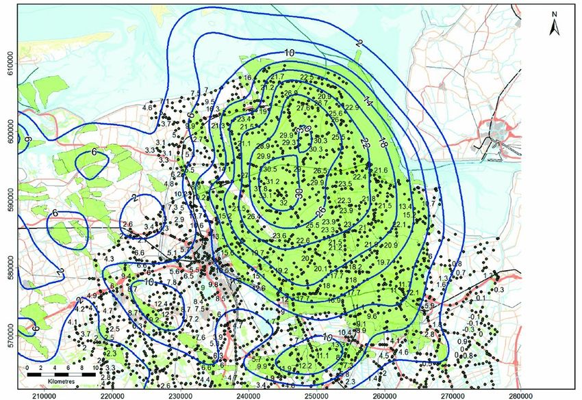
Western Europe (NAM B.V. 2016). Figure 15 shows measured and modelled subsidence
values of the Ems-Dollard region from 1972 to 2013 that were collected within the con-
tinuous monitoring process of the gas field (NAM B.V. 2015). It can be seen that the sub-
sidence reaches into the Ems estuary, even though only with small absolute values ranging
from approximately two to 22 cm, mostly in the area of Paapsand, a tidal flat west of the
navigational channel of the Ems. Subsidence from neighbouring German gas fields is not
included, as there is no monitoring program collecting data. Besides that, output volumes
from the German gas fields are significantly smaller than those from the Groningen gas
field (LBEG 2018).
The subsidence values were transferred into a TIN and subtracted from the depth of
the model grid in order to simulate differences to the control run.
Figure 15: Measured and modelled subsidence values in the Ems-Dollard region for the period
1972–2013. Green areas show gas fields, black dots measured subsidence at benchmarks and blue
lines contour-lines of modelled subsidence (NAM B.V. 2016).Die Küste, 89, 2021 https://doi.org/10.18171/1.089108
Figure 16: Model differences of bathymetry (red) on top overall bathymetry (left) and mean tidal
range values (right) for the control run minus the setup of subsidence values from gas extraction
in the gas field of Groningen. Mind the different scale in comparison to the other figures.
The results show that the influence from gas extraction in the Groningen gas field on single
tidal characteristics in the Ems estuary remains small in comparison to the impact it has on
the vertical land movement. The major part of the differences is below one cm (see Figure
16, right panel). The figure only shows results for mean tidal high-water conditions, because
the greatest subsidence occurs in areas that fall dry during low water.
4 Summary
The setup and application of a cross-scale numerical model to analyse the influence of
morphodynamical and man-made changes in the estuarine zones of the Lower Saxonian
coast on tidal dynamics in adjacent regions was introduced.
Reproductions of morphological states of past and present times have been used to evalu-
ate differences of the tidal regimes and visualize the reach of these changes into unmodified
regions of the model. The results show that local changes of the bathymetry can influence
the tidal regime even far offside the place of action, especially in the leeward direction of
the tidal wave propagation.
The results give an estimate of the contribution of historically large estuarine river con-
struction measures to tidal regime changes. The lack of historical data requires several as-
sumptions in the model and boundary conditions to be made.
The results give a good impression of the man-made contribution to observed long-
term trends in mean high and low water measurements, which is a new and relevant con-
tribution to the interpretation of those data in the context of mean sea level rise and climate
change driven effects.
5 Acknowledgements
We would like to thank our project partners from the Research Institute for Water and
Environment at the University of Siegen and the Institute of Coastal Research at the
Helmholtz-Zentrum Geesthacht for the collaboration and their contributions. ALADYN-CDie Küste, 89, 2021 https://doi.org/10.18171/1.089108 is funded by the German Federal Ministry of Education and Research (BMBF) under the reference 03F0756C. 6 References Ateljevich, E; Zhang, Y.; Nam, Kijin: Hydraulic Structures in SELFE. California Depart- ment of Water Resources, 2014. BUND: Fahrwasservertiefungen der Unter- und Außenweser. Bund für Umwelt und Na- turschutz Deutschland, Landesverband Bremen. Retrieved on Nov. 2018: http://ar- chiv.bund-bremen.net/fileadmin/bundgruppen/bcmslvbremen/naturschutz/weserv- ertiefung/Weservertiefungen_UEbersichtstabelle.pdf. DWD: ICON (Icosahedral Nonhydrostatic) Model, Deutscher Wetterdienst, Offenbach. Retrieved on Jun. 2018: https://www.dwd.de/SharedDocs/downloads/DE/modelldoku- mentationen/nwv/icon/icon_dbbeschr_aktuell.pdf?view=nasPublication&nn=495490 Elsebach, J.; Kaiser, R.; Niemeyer, H. D.: Identifikation von erheblich veränderten Gewäs- serbereichen in der Tideweser. Untersuchungsbericht der NLWKN Forschungsstelle Küste 05/2007, Norderney, 2007 (unpublished). EasyGSH-DB: Erstellung anwendungsorientierter synoptischer Referenzdaten zur Geo- morphologie, Sedimentologie und Hydrodynamik in der Deutschen Bucht (EasyGSH- DB). Retrieved on Apr. 2018: https://wwwmdi-de.baw.de/easygsh EMODnet: European Marine Observation Data Network. Retrieved on Jan. 2017: http://www.emodnet.eu/bathymetry FES: Finite Element Solution Global Tide Model 2014. FES2014 was produced by Noveltis, Legos and CLS Space Oceanography Division and distributed by Aviso, with support from Cnes. Retrieved on Okt. 2017: http://www.aviso.altimetry.fr/ Fokker, P. A.; van Leijen, F. J.; Orlic, B.; van der Marel, H.;Hanssen, R. F.: Subsidence in the Dutch Wadden Sea. In: Netherlands Journal of Geosciences, 97–3, 129–181, https://doi.org/10.1017/njg.2018.9, 2018. Franzius, L.: Die Korrektion der Unterweser. Bremische Deputation für die Unterweser- korrektion, Bremen, 1888. Haigh, I. D., Pickering, M. D., Green, J. A. M., Arbic, B. K., Arns, A., Dangendorf, S., et al.: The tides they are a-changin’: A comprehensive review of past and future nonastro- nomical changes in tides, their driving mechanisms and future implications. In: Reviews of Geophysics, 57, https://doi.org/10.1029/2018RG000636, 2020. Herrling, G.; Niemeyer, H. D.: Reconstruction of the historical tidal regime of the Ems- Dollard estuary prior to significant human changes by applying mathematical modeling. HARBASINS Report, https://www.nlwkn.niedersachsen.de/download/70706, 2007a. Herrling, G.; Niemeyer, H. D.: Long-term Spatial Development of Habitats in the Ems- Dollard Estuary. HARBASINS Report, https://www.nlwkn.niedersachsen.de/down- load/7070, 2007b.
Die Küste, 89, 2021                                           https://doi.org/10.18171/1.089108

Herrling, G.; Niemeyer, H. D.: Comparison of the hydrodynamic regime of 1937 and 2005
in the Ems-Dollard estuary by applying mathematical modeling. HARBASINS Report,
https://www.nlwkn.niedersachsen.de/download/70703, 2008.
Herrling, G.; Elsebach, J.; Ritzmann, A.: Evaluation of Changes in the Tidal Regime of the
Ems-Dollard and Lower Weser Estuaries by Mathematical Modelling. In: Die Küste, 81,
2014.
Hensen, W.: Modellversuche für die untere Ems. Mitteilungen der Hannoverschen Ver-
suchsanstalt für Grundbau und Wasserbau. Franzius-Institut der Technischen Hochschule
Hannover. Hannover, 1954.
Homeier, H.; Stephan H.-J.; Niemeyer, H. D.: Historisches Kartenwerk Niedersächsische
Küste der Forschungsstelle Küste. Berichte der Forschungsstelle Küste. Band 43/2010,
Norderney, 2010.
Hubert, K.; Wurpts, A.; Berkenbrink, C.: Modelling the Impact of Estuarine and Coastal
Morphological Changes on Tidal Dynamics in the German Bight. In: E-proceedings of the
38th IAHR World Congress September 1–6, 2019, Panama City, https://doi.org/10.3850/
38WC092019-0799, 2019.
HPA: Deutsches Gewässerkundliches Jahrbuch Elbegebiet Teil III 2014. Hamburg Port
Authority, Hamburg, 2017.
Lang, A. W.: Historisches Seekartenwerk der Deutschen Bucht. No 78 Grapow, Jade-,
Weser- und Elbmündungen, Berlin 1870. Karl Wachtholtz Verlag, Neumünster 1973.
LBEG: Erdöl und Erdgas in der Bundesrepublik Deutschland 2017. Landesamt für Berg-
bau, Energie und Geologie. Hannover, 2018.
NAM B.V.: Bodemdaling door aardgaswinning. NAM-velden in Groningen, Friesland en
het noorden van Drenthe. Status rapport 2015 en Prognose tot het jaar 2080. Nederlandse
Aardolie Maatschappij B.V., Assen, 2015.
NAM B.V.: Winningsplan Groningen Gasveld 2016, 2016. https://www.nam.nl/alge-
meen/mediatheek-en-downloads/winningsplan-2016/_jcr_content/par/tex-
timage_996696702.stream/1461000524569/1d3f1162f0dbba3f15b8bbc2c7087224fb413e
e1/winningsplan-groningen-2016.pdf, Request: Okt. 2017.
Niemeyer, H. D.; Kaiser, R.: Mittlere Tidewasserstände. In: Umweltatlas Wattenmeer. Band
2: Wattenmeer zwischen Elb- und Emsmündung. Nationalparkverwaltung Niedersächsi-
sches Wattenmeer, Umweltbundesamt. Wilhelmshaven, Berlin, 1999.
Niemeyer, H. D.: Prüfung der Sturmflutsicherheit in Brake zwischen Weserlust und Haus
Linne. NLÖ Forschungsstelle Küste, Norderney, 2000 (unpublished).
NLWKN: Deutsches Gewässerkundliches Jahrbuch Weser- und Emsgebiet 2015. Nieder-
sächsischer Landesbetrieb für Wasserwirtschaft, Küsten- und Naturschutz, Norden, 2018.
Portal Tideweser: Weseranpassung. Wasserstraßen- und Schifffahrtsverwaltung. Retrieved
on Jul. 2019: https://www.kuestendaten.de/Tideweser/DE/Projekte/Weseranpassung/
Weseranpassung-node.html
Schureman, Paul: Manual of Harmonic Analysis and Prediction of Tides. Special Publica-
tions No. 98. U.S. Department of Commerce, 1940.
Die Küste, 89, 2021                                           https://doi.org/10.18171/1.089108

See- und Ozeanhandbücher: Nr. 2006: Nordsee, östlicher Teil. Von Hanstholm bis
Terschelling. Deutsches Hydrographisches Institut, Hamburg, 1958.
Verboom, G. K.; de Ronde, J. G.;van Dijk, R. P.: A fine grid tidal flow and storm surge
model of the North Sea. In: Continent. Shelf Res.,12, 1991.
Zhang, Y.; Ateljevich, E.; Yu, H-C.; Wu, C-H.; Yu, J. C. S.: A new vertical coordinate sys-
tem for a 3D unstructured-grid model. In: Ocean Modelling, 85, 16–31, 2015.
Zhang, Y.; Ye, F.; Stanev, E. V.; Grashorn, S.: Seamless cross-scale modeling with
SCHISM. In: Ocean Modelling, 102, 64–81, 2016.
You can also read