META-LEARNING WITH LATENT EMBEDDING OPTIMIZATION
←
→
Page content transcription
If your browser does not render page correctly, please read the page content below
Published as a conference paper at ICLR 2019

                                         M ETA -L EARNING WITH
                                         L ATENT E MBEDDING O PTIMIZATION
                                          Andrei A. Rusu, Dushyant Rao, Jakub Sygnowski, Oriol Vinyals,
                                          Razvan Pascanu, Simon Osindero & Raia Hadsell
                                          DeepMind, London, UK
                                          {andreirusu, dushyantr, sygi, vinyals,
                                          razp, osindero, raia}@google.com
arXiv:1807.05960v3 [cs.LG] 26 Mar 2019

                                                                                      A BSTRACT

                                                  Gradient-based meta-learning techniques are both widely applicable and profi-
                                                  cient at solving challenging few-shot learning and fast adaptation problems. How-
                                                  ever, they have practical difficulties when operating on high-dimensional param-
                                                  eter spaces in extreme low-data regimes. We show that it is possible to bypass
                                                  these limitations by learning a data-dependent latent generative representation
                                                  of model parameters, and performing gradient-based meta-learning in this low-
                                                  dimensional latent space. The resulting approach, latent embedding optimization
                                                  (LEO), decouples the gradient-based adaptation procedure from the underlying
                                                  high-dimensional space of model parameters. Our evaluation shows that LEO
                                                  can achieve state-of-the-art performance on the competitive miniImageNet and
                                                  tieredImageNet few-shot classification tasks. Further analysis indicates LEO is
                                                  able to capture uncertainty in the data, and can perform adaptation more effec-
                                                  tively by optimizing in latent space.

                                         1    I NTRODUCTION

                                         Humans have a remarkable ability to quickly grasp new concepts from a very small number of ex-
                                         amples or a limited amount of experience, leveraging prior knowledge and context. In contrast,
                                         traditional deep learning approaches (LeCun et al., 2015; Schmidhuber, 2015) treat each task inde-
                                         pendently and hence are often data inefficient – despite providing significant performance improve-
                                         ments across the board, such as for image classification (Simonyan & Zisserman, 2014; He et al.,
                                         2016), reinforcement learning (Mnih et al., 2015; Silver et al., 2017), and machine translation (Cho
                                         et al., 2014; Sutskever et al., 2014). Just as humans can efficiently learn new tasks, it is desirable for
                                         learning algorithms to quickly adapt to and incorporate new and unseen information.
                                         Few-shot learning tasks challenge models to learn a new concept or behaviour with very few exam-
                                         ples or limited experience (Fei-Fei et al., 2006; Lake et al., 2011). One approach to address this class
                                         of problems is meta-learning, a broad family of techniques focused on learning how to learn or to
                                         quickly adapt to new information. More specifically, optimization-based meta-learning approaches
                                         (Ravi & Larochelle, 2017; Finn et al., 2017) aim to find a single set of model parameters that can
                                         be adapted with a few steps of gradient descent to individual tasks. However, using only a few
                                         samples (typically 1 or 5) to compute gradients in a high-dimensional parameter space could make
                                         generalization difficult, especially under the constraint of a shared starting point for task-specific
                                         adaptation.
                                         In this work we propose a new approach, named Latent Embedding Optimization (LEO), which
                                         learns a low-dimensional latent embedding of model parameters and performs optimization-based
                                         meta-learning in this space. Intuitively, the approach provides two advantages. First, the initial
                                         parameters for a new task are conditioned on the training data, which enables a task-specific starting
                                         point for adaptation. By incorporating a relation network into the encoder, this initialization can
                                         better consider the joint relationship between all of the input data. Second, by optimizing in the
                                         lower-dimensional latent space, the approach can adapt the behaviour of the model more effectively.
                                         Further, by allowing this process to be stochastic, the ambiguities present in the few-shot data regime
                                         can be expressed.

                                                                                             1
Published as a conference paper at ICLR 2019

We demonstrate that LEO achieves state-of-the-art results on both the miniImageNet and
tieredImageNet datasets, and run an ablation study and further analysis to show that both conditional
parameter generation and optimization in latent space are critical for the success of the method.
Source code for our experiments is available at https://github.com/deepmind/leo.

2     M ODEL
2.1   P ROBLEM D EFINITION

We define the N -way K-shot problem using the episodic formulation of Vinyals et al. (2016). Each
task instance Ti is a classification problem sampled from a task distribution p(T ). The tasks are
divided into a training meta-set S tr , validation meta-set S val , and test meta-set S test , each with a
disjoint set of target classes (i.e., a class seen during testing is not seen during training). The valida-
tion meta-set is used for model selection, and the testing meta-set is used only for final evaluation.
Each task instance Ti ∼ p (T ) is composed of a training set Dtr and validation set Dval , and
only contains N classes randomly selected from the appropriate meta-set (e.g. for a task instance
in the training meta-set,
                         the classes are a subset of those available in S tr ). In most setups, the
training set Dtr = (xkn , ynk ) | k = 1 . . . K; n = 1 . . . N contains K samples for each class. The
validation set Dval can contain several other samples from the same classes, providing an estimate of
generalization performance on the N classes for this problem instance. We note that the validation
set of a problem instance Dval (used to optimize a meta-learning objective) should not be confused
with the held-out validation meta-set S val (used for model selection).

2.2   M ODEL -AGNOSTIC M ETA -L EARNING

Model-agnostic meta-learning (MAML) (Finn et al., 2017) is an approach to optimization-based
meta-learning that is related to our work. For some parametric model fθ , MAML aims to find a
single set of parameters θ which, using a few optimization steps, can be successfully adapted to any

novel task sampled from the same distribution. For a particular task instance Ti = Dtr , Dval ,
the parameters are adapted to task-specific model parameters θi0 by applying some differentiable
function, typically an update rule of the form:
                                           θi0 = G θ, Dtr ,

                                                                                                  (1)
where G is typically implemented as a step of gradient descent on the few-shot training set Dtr ,
θi0 = θ − α∇θ Ltr
               Ti (fθ ). Generally, multiple sequential adaptation steps can be applied. The learning
rate α can also be meta-learned concurrently, in which case we refer to this algorithm as Meta-
SGD (Li et al., 2017). During meta-training, the parameters θ are updated by back-propagating
through the adaptation procedure, in order to reduce errors on the validation set Dval :
                                                  X
                                                         Lval

                                  θ ← θ − η∇θ              Ti  fθi0                               (2)
                                                   Ti ∼p(T )

The approach includes the main ingredients of optimization-based meta-learning with neural net-
works: initialization is done by maintaining an explicit set of model parameters θ; the adaptation
procedure, or “inner loop”, takes θ as input and returns θi0 adapted specifically for task instance Ti ,
by iteratively using gradient descent (Eq. 1); and termination, which is handled simply by choos-
ing a fixed number of optimization steps in the “inner loop”. MAML updates θ by differentiating
through the “inner loop” in order to minimize errors of instance-specific adapted models fθi0 on the
corresponding validation set (Eq. 2). We refer to this process as the “outer loop” of meta-learning.
In the next section we use the same stages to describe Latent Embedding Optimization (LEO).

2.3   L ATENT E MBEDDING O PTIMIZATION FOR M ETA -L EARNING

The primary contribution of this paper is to show that it is possible, and indeed beneficial, to de-
couple optimization-based meta-learning techniques from the high-dimensional space of model
parameters. We achieve this by learning a stochastic latent space with an information bottleneck,
conditioned on the input data, from which the high-dimensional parameters are generated.

                                                    2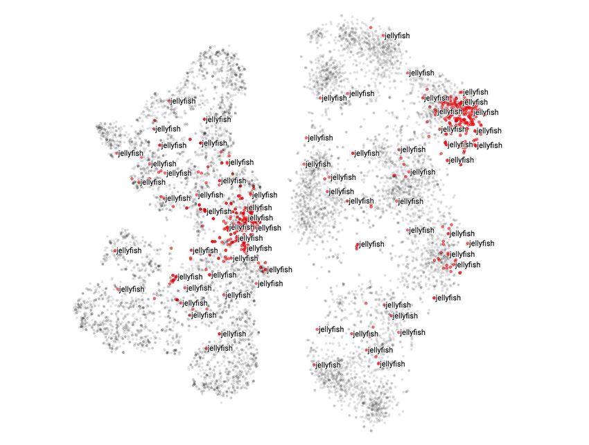
Published as a conference paper at ICLR 2019

Algorithm 1 Latent Embedding Optimization
Require: Training meta-set S tr ∈ T
Require: Learning rates α, η
 1: Randomly initialize φe , φr , φd
 2: Let φ = {φe , φr , φd , α}
 3: while not converged do
 4:   for number of tasks in batch do
 5:      Sample task instance    Ti ∼ S tr
         Let Dtr , Dval = Ti

 6:
 7:      Encode Dtr to z using gφe and gφr
 8:      Decode z to initial params θi using gφd
 9:      Initialize z0 = z, θi0 = θi
10:      for number of adaptation steps do
11:         Compute training loss Ltr  Ti fθi0
                                           0
12:         Perform gradient step w.r.t.
              0     0            tr
                                         z:
            z ← z − α∇z0 LTi fθi0
13:         Decode z0 to obtain θi0 using gφd
14:      end for                                            Figure 1: High-level intuition for LEO. While
         Compute validation loss Lval

15:                                  Ti fθi0                MAML operates directly in a high dimensional
16:   end for                                               parameter space Θ, LEO performs meta-learning
17:   Perform gradient Pstep w.r.t φ:                      within a low-dimensional latent space Z, from
      φ ← φ − η∇φ Ti Lval      Ti fθi0                      which the parameters are generated.
18: end while

                                                                                    optimized in inner loop

                                                                                    optimized in outer loop

                                                                                              Inference
                                                  Decoder
                       Encoder

                                 Relation
                                   Net

                                                                                              Inner loop
                                                                                             optimization

                                     Figure 2: Overview of the architecture of LEO.

Instead of explicitly instantiating and maintaining a unique set of model parameters θ, as in MAML,
we learn a generative distribution of model parameters which serves the same purpose. This is a nat-
ural extension: we relax the requirement of finding a single optimal θ∗ ∈ Θ to that of approximating
a data-dependent conditional probability distribution over Θ, which can be more expressive. The
choice of architecture, composed of an encoding process, and decoding (or parameter generation)
process, enables us to perform the MAML gradient-based adaptation steps (or “inner loop”) in the
learned, low-dimensional embedding space of the parameter generative model (Figure 1).

2.3.1      M ODEL OVERVIEW
The high-level operation is then as follows (Algorithm 1). First, given a task instance Ti , the inputs
{xkn } are passed through a stochastic encoder to produce a latent code z, which is then decoded
to parameters θi using a parameter generator1 . Given these instantiated model parameters, one
or more adaptation steps are applied in the latent space, by differentiating the loss with respect to
z, taking a gradient step to get z0 , decoding new model parameters, and obtaining the new loss.
Finally, optimized codes are decoded to produce the final adapted parameters θi0 , which can be used
to perform the task, or compute the task-specific meta-loss. In this way, LEO incorporates aspects of
model-based and optimization-based meta-learning, producing parameters that are first conditioned
on the input data and then adapted by gradient descent.

   1
       Note that we omit the task subscript i from latent code z and input data xkn for clarity.

                                                            3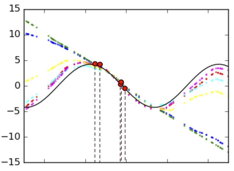
Published as a conference paper at ICLR 2019

Figure 2 shows the architecture of the resulting network. Intuitively, the decoder is akin to a gener-
ative model, mapping from a low-dimensional latent code to a distribution over model parameters.
The encoding process ensures that the initial latent code and parameters before gradient-based adap-
tation are already data-dependent. This encoding process also exploits a relation network that allows
the latent code to be context-dependent, considering the pairwise relationship between all classes in
the problem instance. In the following sections, we explain the LEO procedure more formally.

2.3.2      I NITIALIZATION : G ENERATING PARAMETERS C ONDITIONED ON A F EW E XAMPLES
The first stage is to instantiate the model parameters that will be adapted to each task instance.
Whereas MAML explicitly maintains a single set of model parameters, LEO utilises a data-
dependent latent encoding which is then decoded to generate the actual initial parameters. In what
follows, we describe an encoding scheme which leverages a relation network to map the few-shot
examples into a single latent vector. This design choice allows the approach to consider context
when producing a parameter initialization. Intuitively, decision boundaries required for fine-grained
distinctions between similar classes might need to be different from those for broader classification.

Encoding The encoding process involves a simple feed-forward mapping of each data point, fol-
lowed by a relation network that considers the pair-wise relationship between the data in the problem
instance. The overall encoding process is defined in  Eq. 3, and proceeds as follows. First, each ex-
ample from a problem instance Ti = Dtr , Dval ∼ p (T ) is processed by an encoder network
gφe : Rnx → Rnh , which maps from input space to a code in an intermediate hidden-layer code
space H. Then, codes in H corresponding to different training examples are concatenated pair-wise
(resulting in (N K)2 pairs in the case of K-shot classification) and processed by a relation network
gφr , in a similar fashion to Oreshkin et al. (2018) and Sung et al. (2017). The (N K)2 outputs are
grouped by class and averaged within each group to obtain the (2 × N ) parameters of a probability
distribution in a low-dimensional space Z = Rnz , where nz  dim(θ), for each of the N classes.
                                                                                    k k
Thus, given the K-shot training samples corresponding to a class n: Dntr =           xn , yn | k =
1 . . . K the encoder gφe and relation network gφr together parameterize a class-conditional mul-
tivariate Gaussian distribution with a diagonal covariance, which we can sample from in order to
output a class-dependent latent code zn ∈ Z as follows:
                                            K     N   K
                                       1 X X X
                    µen , σ en                                          kn           km

                                 =                         gφ r
                                                                  gφe
                                                                      x n    , gφe
                                                                                   x m
                                     N K2
                                           kn =1 m=1 km =1

                                     zn ∼ q zn |Dntr = N µen , diag(σ en 2 )

                                                                                                    (3)

Intuitively, the encoder and relation network define a stochastic mapping from one or more class
examples to a single code in the latent embedding space Z corresponding to that class. The final
latent code can be obtained as the concatenation of class-dependent codes: z = [z1 , z2 , . . . , zN ].

Decoding Without loss of generality, for few-shot classification, we can use the class-specific
latent codes to instantiate just the top layer weights of the classifier. This allows the meta-learning
in latent space to modulate the important high-level parameters of the classifier, without requiring the
generator to produce very high-dimensional parameters. In this case, fθi0 is a N -way linear softmax
classifier, with model parameters θi0 = wn | n = 1 . . . N , and each xkn can be either the raw input


or some learned representation2 . Then, given the latent codes zn ∈ Z, n = 1 . . . N , the decoder
function gφd : Z → Θ is used to parameterize a Gaussian distribution with diagonal covariance in
model parameter space Θ, from which we can sample class-dependent parameters wn :
                                          µdn , σ dn
                                                = gφd (zn )
                                                                  2

                                 wn ∼ p (w|zn ) = N µdn , diag(σ dn )                               (4)

In other words, codes zn are mapped independently to the top-layer parameters θi of a softmax
classifier using the decoder gφd , which is essentially a stochastic generator of model parameters.
   2
       As before, we omit the task subscript i from wn for clarity.

                                                         4
Published as a conference paper at ICLR 2019

2.3.3     A DAPTATION BY L ATENT E MBEDDING O PTIMIZATION (LEO) (T HE “I NNER L OOP ”)
Given the decoded parameters, we can then define the “inner loop” classification loss using the
cross-entropy function, as follows:
                                           X h                          N
                                                                       X             i
                             Ltr                                             ewj ·x

                              Ti fθi =                − wy · x + log                                  (5)
                                         (x,y)∈D tr                    j=1

It is important to note that the decoder gφd is a differentiable mapping between the latent space Z and
the higher-dimensional model parameter space Θ. Primarily, this allows gradient-based optimization
of the latent codes with respect to the training loss, with z0n = zn − α∇zn Ltr
                                                                              Ti . The decoder gφd will
convert adapted latent codes z0n to effective model parameters θi0 for each adaptation step, which
can be repeated several times, as in Algorithm 1. In addition, by backpropagating errors through the
decoder, the encoder and relation net can learn to provide a data-conditioned latent encoding z that
produces an appropriate initialization point θi for the classifier model.

2.3.4     M ETA -T RAINING S TRATEGY (T HE “O UTER L OOP ”)
For each task instance Ti , the initialization and adaptation procedure produce a new classifier fθi0
tailored to the training set Dtr of the instance, which we can then evaluate on the validation set of that
instance Dval . During meta-training we use that evaluation to differentiate through the “inner loop”
and update the encoder, relation, and decoder network parameters: φe , φr , and φd . Meta-training is
performed by minimizing the following objective:
               X h                                                                           i
                                                                                 0
                       Lval                          tr                                    2

     min                Ti fθi0 + βDKL q(zn |Dn )||p(zn ) + γ||stopgrad(zn ) − zn ||2 + R              (6)
    φe ,φr ,φd
                 Ti ∼p(T )

where p(zn ) = N (0, I). Similar to the loss defined in (Higgins et al., 2017) we use a weighted
KL-divergence term to regularize the latent space and encourage the generative model to learn a
disentangled embedding, which should also simplify the LEO “inner loop” by removing correlations
between latent space gradient dimensions. The third term in Eq. (6) encourages the encoder and
relation net to output a parameter initialization that is close to the adapted code, thereby reducing
the load of the adaptation procedure if possible.
L2 regularization was used with all weights of the model, as well as a soft, layer-wise orthogonality
constraint on decoder network weights, which encourages the dimensions of the latent code as well
as the decoder network to be maximally expressive. In the case of linear encoder, relation, and
decoder networks, and assuming that Cd is the correlation matrix between rows of φd , then the
regularization term takes the following form:

                       R = λ1 ||φe ||22 + ||φr ||22 + ||φd ||22 + λ2 ||Cd − I||2                  (7)

2.3.5     B EYOND C LASSIFICATION AND L INEAR O UTPUT L AYERS
Thus far we have used few-shot classification as a working example to highlight our proposed
method, and in this domain we generate only a single linear output layer. However, our approach can
be applied to any model fθi which maps observations to outputs, e.g. a nonlinear MLP or LSTM,
by using a single latent code z to generate the entire parameter vector θi with an appropriate de-
coder. In the general case, z is conditioned on Dtr by passing both inputs and labels to the encoder.
Furthermore, the loss LTi is not restricted to be a classification loss, and can be replaced by any
differentiable loss function which can be computed on Dtr and Dval sets of a task instance Ti .

3     R ELATED W ORK
The problem of few-shot adaptation has been approached in the context of fast weights (Hinton &
Plaut, 1987; Ba et al., 2016), learning-to-learn (Schmidhuber, 1987; Thrun & Pratt, 1998; Hochre-
iter et al., 2001; Andrychowicz et al., 2016), and through meta-learning. Many recent approaches to
meta-learning can be broadly categorized as metric-based methods, which focus on learning simi-
larity metrics for members of the same class (e.g. Koch et al., 2015; Vinyals et al., 2016; Snell et al.,

                                                        5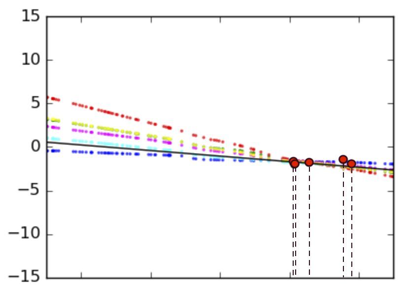
Published as a conference paper at ICLR 2019

2017); memory-based methods, which exploit memory architectures to store key training examples
or directly encode fast adaptation algorithms (e.g. Santoro et al., 2016; Ravi & Larochelle, 2017);
and optimization-based methods, which search for parameters that are conducive to fast gradient-
based adaptation to new tasks (e.g. Finn et al., 2017; 2018).
Related work has also explored the use of one neural network to produce (some fraction of) the
parameters of another (Ha et al., 2016; Krueger et al., 2017), with some approaches focusing on
the goal of fast adaptation. Munkhdalai et al. (2017) meta-learn an algorithm to change additive
biases across deep networks conditioned on the few-shot training samples. In contrast, Gidaris
& Komodakis (2018) use an attention kernel to output class conditional mixing of linear output
weights for novel categories, starting from a pre-trained deep model. Qiao et al. (2017) learn to
output top linear layer parameters from the activations provided by a pre-trained feature embedding,
but they do not make use of gradient-based adaptation. None of the aforementioned approaches
to fast adaptation explicitly learn a probability distribution over model parameters, or make use of
latent variable generative models to characterize it.
Approaches which use optimization-based meta-learning include MAML (Finn et al., 2017) and
REPTILE (Nichol & Schulman, 2018). While MAML backpropagates the meta-loss through the
“inner loop”, REPTILE simplifies the computation by incorporating an L2 loss which updates the
meta-model parameters towards the instance-specific adapted models. These approaches use the full,
high-dimensional set of model parameters within the “inner loop”, while Lee & Choi (2018) learn
a layer-wise subspace in which to use gradient-based adaptation. However, it is not clear how these
methods scale to large expressive models such as residual networks (especially given the uncertainty
in the few-shot data regime), since MAML is prone to overfitting (Mishra et al., 2018). Recognizing
this issue, Zhou et al. (2018) train a deep input representation, or “concept space”, and use it as
input to an MLP meta-learner, but perform gradient-based adaptation directly in its parameter space,
which is still comparatively high-dimensional. As we will show, performing adaptation in latent
space to generate a simple linear layer can lead to superior generalization.
Probabilistic meta-learning approaches such as those of Bauer et al. (2017) and Grant et al. (2018)
have shown the advantages of learning Gaussian posteriors over model parameters. Concurrently
with our work, Kim et al. (2018) and Finn et al. (2018) propose probabilistic extensions to MAML
that are trained using a variational approximation, using simple posteriors. However, it is not im-
mediately clear how to extend them to more complex distributions with a more diverse set of tasks.
Other concurrent works have introduced deep parameter generators (Lacoste et al., 2018; Wu et al.,
2018) that can better capture a wider distribution of model parameters, but do not employ gradient-
based adaptation. In contrast, our approach employs both a generative model of parameters, and
adaptation in a low-dimensional latent space, aided by a data-dependent initialization.
Finally, recently proposed Neural Processes (Garnelo et al., 2018a;b) bear similarity to our work:
they also learn a mapping to and from a latent space that can be used for few-shot function estima-
tion. However, coming from a Gaussian processes perspective, their work does not perform “inner
loop” adaptation and is trained by optimizing a variational objective.

4     E VALUATION
We evaluate the proposed approach on few-shot regression and classification tasks. This evaluation
aims to answer the following key questions: (1) Is LEO capable of modeling a distribution over
model parameters when faced with uncertainty? (2) Can LEO learn from multimodal task distri-
butions and is this reflected in ambiguous problem instances, where multiple distinct solutions are
possible? (3) Is LEO competitive on large-scale few-shot learning benchmarks?

4.1   F EW- SHOT R EGRESSION

To answer the first two questions we adopt the simple regression task of Finn et al. (2018). 1D
regression problems are generated in equal proportions using either a sine wave with random am-
plitude and phase, or a line with random slope and intercept. Inputs are sampled randomly, creating
a multimodal task distribution. Crucially, random Gaussian noise with standard deviation 0.3 is
added to regression targets. Coupled with the small number of training samples (5-shot), the task is
challenging for 2 main reasons: (1) learning a distribution over models becomes necessary, in order

                                                 6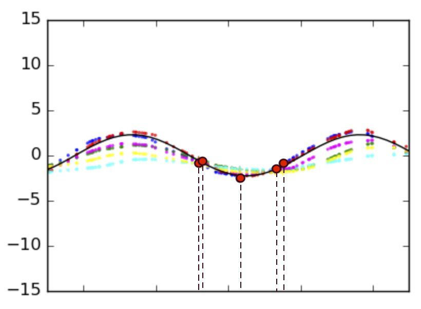
Published as a conference paper at ICLR 2019

to account for the uncertainty introduced by noisy labels; (2) problem instances may be likely under
both modes: in some cases a sine wave may fit the data as well as a line. Faced with such ambiguity,
learning a generative distribution of model parameters should allow several different likely models
to be sampled, in a similar way to how generative models such as VAEs can capture different modes
of a multimodal data distribution.
We used a 3-layer MLP as the underlying model architecture of fθ , and we produced the entire
parameter tensor θ with the LEO generator, conditionally on Dtr , the few-shot training inputs con-
catenated with noisy labels. For further details, see Appendix A.

                      (a)                      (b)                       (c)                       (d)

Figure 3: Meta-learning with LEO of a multimodal task distribution with sines and lines, using
5-shot regression with noisy targets. Our model outputs a distribution of possible solutions, which
is also multimodal in ambiguous cases. True regression targets are plotted in black, while the 5
training examples are highlighted with red circles and vertical dashed lines. Several samples from
our model are plotted with dotted lines (best seen in color).

In Figure 3 we show samples from a single model trained on noisy sines and lines, with true regres-
sion targets in black and training samples marked with red circles and vertical dashed lines. Plots (a)
and (b) illustrate how LEO captures some of the uncertainty in ambiguous problem instances within
each mode, especially in parts of the input space far from any training samples. Conversely, in parts
which contain data, models fit the regression target well. Interestingly, when both sines and lines
could explain the data, as shown in panels (c) and (d), we see that LEO can sample very different
models, from both families, reflecting its ability to represent parametric uncertainty appropriately.

4.2     F EW- SHOT C LASSIFICATION

In order to answer the final question we scale up our approach to 1-shot and 5-shot classification
problems defined using two commonly used ImageNet subsets.

4.2.1    DATASETS
The miniImageNet dataset (Vinyals et al., 2016) is a subset of 100 classes selected randomly from
the ILSVRC-12 dataset (Russakovsky et al., 2014) with 600 images sampled from each class. Fol-
lowing the split proposed by Ravi & Larochelle (2017), the dataset is divided into training, valida-
tion, and test meta-sets, with 64, 16, and 20 classes respectively.
The tieredImageNet dataset (Ren et al., 2018) is a larger subset of ILSVRC-12 with 608 classes
(779,165 images) grouped into 34 higher-level nodes in the ImageNet human-curated hierarchy
(Deng et al., 2009a). This set of nodes is partitioned into 20, 6, and 8 disjoint sets of training,
validation, and testing nodes, and the corresponding classes form the respective meta-sets. As argued
in Ren et al. (2018), this split near the root of the ImageNet hierarchy results in a more challenging,
yet realistic regime with test classes that are less similar to training classes.

4.2.2    P RE - TRAINED F EATURES
Two potential difficulties of using LEO to instantiate parameters with a generator network are:
(1) modeling distributions over very high-dimensional parameter spaces; and (2) requiring meta-
learning (and hence, gradient computation in the inner loop) to be performed with respect to a
high-dimensional input space. We address these issues by pre-training a visual representation of the
data and then using the generator to instantiate the parameters for the final layer - a linear softmax
classifier operating on this representation. We train a 28-layer Wide Residual Network (WRN-28-
10) (Zagoruyko & Komodakis, 2016a) with supervised classification using only data and classes

                                                     7
Published as a conference paper at ICLR 2019
from the training meta-set. Recent state-of-the-art approaches use the penultimate layer representa-
tion (Zhou et al., 2018; Qiao et al., 2017; Bauer et al., 2017; Gidaris & Komodakis, 2018); however,
we choose the intermediate feature representation in layer 21, given that higher layers tend to special-
ize to the training distribution (Yosinski et al., 2014). For details regarding the training, evaluation,
and network architectures, see Appendix B.
4.2.3 F INE - TUNING
Following the LEO adaptation procedure (Algorithm 1) we also use fine-tuning3 by performing a
few steps of gradient-based adaptation directly in parameter space using the few-shot set Dtr . This is
similar to the adaptation procedure of MAML, or Meta-SGD (Li et al., 2017) when the learning rates
are learned, with the important difference that starting points of fine-tuning are custom generated by
LEO for every task instance Ti . Empirically, we find that fine-tuning applies a very small change to
the parameters with only a slight improvement in performance on supervised classification tasks.
4.3 R ESULTS
miniImageNet test accuracy
Model
1-shot 5-shot
Matching networks (Vinyals et al., 2016) 43.56 ± 0.84% 55.31 ± 0.73%
Meta-learner LSTM (Ravi & Larochelle, 2017) 43.44 ± 0.77% 60.60 ± 0.71%
MAML (Finn et al., 2017) 48.70 ± 1.84% 63.11 ± 0.92%
LLAMA (Grant et al., 2018) 49.40 ± 1.83% -
REPTILE (Nichol & Schulman, 2018) 49.97 ± 0.32% 65.99 ± 0.58%
PLATIPUS (Finn et al., 2018) 50.13 ± 1.86% -
Meta-SGD (our features) 54.24 ± 0.03% 70.86 ± 0.04%
SNAIL (Mishra et al., 2018) 55.71 ± 0.99% 68.88 ± 0.92%
(Gidaris & Komodakis, 2018) 56.20 ± 0.86% 73.00 ± 0.64%
(Bauer et al., 2017) 56.30 ± 0.40% 73.90 ± 0.30%
(Munkhdalai et al., 2017) 57.10 ± 0.70% 70.04 ± 0.63%
DEML+Meta-SGD (Zhou et al., 2018) 4 58.49 ± 0.91% 71.28 ± 0.69%
TADAM (Oreshkin et al., 2018) 58.50 ± 0.30% 76.70 ± 0.30%
(Qiao et al., 2017) 59.60 ± 0.41% 73.74 ± 0.19%
LEO (ours) 61.76 ± 0.08% 77.59 ± 0.12%
tieredImageNet test accuracy
Model
1-shot 5-shot
MAML (deeper net, evaluated in Liu et al. (2018)) 51.67 ± 1.81% 70.30 ± 0.08%
Prototypical Nets (Ren et al., 2018) 53.31 ± 0.89% 72.69 ± 0.74%
Relation Net (evaluated in Liu et al. (2018)) 54.48 ± 0.93% 71.32 ± 0.78%
Transductive Prop. Nets (Liu et al., 2018) 57.41 ± 0.94% 71.55 ± 0.74%
Meta-SGD (our features) 62.95 ± 0.03% 79.34 ± 0.06%
LEO (ours) 66.33 ± 0.05% 81.44 ± 0.09%
Table 1: Test accuracies on miniImageNet and tieredImageNet. For each dataset, the first set of
results use convolutional networks, while the second use much deeper residual networks, predomi-
nantly in conjuction with pre-training.
The classification accuracies for LEO and other baselines are shown in Table 1. LEO sets
the new state-of-the-art performance on the 1-shot and 5-shot tasks for both miniImageNet and
tieredImageNet datasets. We also evaluated LEO on the “multi-view” feature representation used
by Qiao et al. (2017) with miniImageNet, which involves significant data augmentation compared to
the approaches in Table 1. LEO is state-of-the-art using these features as well, with 63.97 ± 0.20%
and 79.49 ± 0.70% test accuracies on the 1-shot and 5-shot tasks respectively.
4.4 A BLATION S TUDY
To assess the effects of different components, we also performed an ablation study, with detailed
results in Table 2. To ensure a fair comparison, all approaches begin with the same pre-trained
3
In this context, “fine-tuning” refers to final adaptation in parameter space, rather than fine-tuning the pre-
trained feature extractor.
4
Uses the ImageNet-200 dataset (Deng et al., 2009b) to train the concept generator.
8Published as a conference paper at ICLR 2019
miniImageNet test accuracy tieredImageNet test accuracy
Model
1-shot 5-shot 1-shot 5-shot
Meta-SGD (our features) 54.24 ± 0.03% 70.86 ± 0.04% 62.95 ± 0.03% 79.34 ± 0.06%
Conditional generator only 60.33 ± 0.11% 74.53 ± 0.11% 65.17 ± 0.15% 78.77 ± 0.03%
Conditional generator + fine-tuning 60.62 ± 0.31% 76.42 ± 0.09% 65.74 ± 0.28% 80.65 ± 0.07%
Previous SOTA 59.60 ± 0.41% 76.70 ± 0.30% 57.41 ± 0.94% 72.69 ± 0.74%
LEO (random prior) 61.01 ± 0.12% 77.27 ± 0.05% 65.39 ± 0.10% 80.83 ± 0.13%
LEO (deterministic) 61.48 ± 0.05% 76.53 ± 0.24% 66.18 ± 0.17% 82.06 ± 0.08%
LEO (no fine-tuning) 61.62 ± 0.15% 77.46 ± 0.12% 66.14 ± 0.17% 80.89 ± 0.11%
LEO (ours) 61.76 ± 0.08% 77.59 ± 0.12% 66.33 ± 0.05% 81.44 ± 0.09%
Table 2: Ablation study and comparison to Meta-SGD. Unless otherwise specified, LEO stands for
using the stochastic generator for latent embedding optimization followed by fine-tuning.
features (Section 4.2.2). The Meta-SGD case performs gradient-based adaption directly in the pa-
rameter space in the same way as MAML, but also meta-learns the inner loop learning rate (as we
do for LEO). The main approach, labeled as LEO in the table, uses a stochastic parameter generator
for several steps of latent embedding optimization, followed by fine-tuning steps in parameter space
(see subsection 4.2.3). All versions of LEO are at or above the previous state-of-the-art on all tasks.
The largest difference in performance is between Meta-SGD and the other cases (all of which ex-
ploit a latent representation of model parameters), indicating that the low-dimensional bottleneck
is critical for this application. The “conditional generator only” case (without adaptation in latent
space) yields a poorer result than LEO, and even adding fine-tuning in parameter space does not
recover performance; this illustrates the efficacy of the latent adaptation procedure. The importance
of the data-dependent encoding is highlighted by the “random prior” case, in which the encoding
process is replaced by the prior p(zn ), and performance decreases. We also find that incorporating
stochasticity can be important for miniImageNet, but not for tieredImageNet, which we hypothesize
is because the latter is much larger. Finally, the fine-tuning steps only yield a statistically signifi-
cant improvement on the 5-shot tieredImageNet task. Thus, both the data-conditional encoding and
latent space adaptation are critical to the performance of LEO.
(a) (b) (c)
Figure 4: t-SNE plot of latent space codes before and after adaptation: (a) Initial codes zn (blue)
and adapted codes z0n (orange); (b) Same as (a) but colored by class; (c) Same as (a) but highlighting
codes zn for validation class “Jellyfish” (left) and corresponding adapted codes z0n (right).
4.5 L ATENT E MBEDDING V ISUALIZATION
To qualitatively characterize the learnt embedding space, we plot codes produced by the relational
encoder before and after the LEO procedure, using a 5-way 1-shot model and 1000 task instances
from the validation meta-set of miniImageNet. Figure 4 shows a t-SNE projection of class condi-
tional encoder outputs zn as well as their respective final adapted versions z0n . If the effect of LEO
were minimal, we would expect latent codes to have roughly the same structure before and after
adaptation. In contrast, Figure 4(a) clearly shows that latent codes change substantially during LEO,
since encoder output codes form a large cluster (blue) to which adapted codes (orange) do not be-
long. Figure 4(b) shows the same t-SNE embedding as (a) colored by class label. Note that encoder
9Published as a conference paper at ICLR 2019
(a) (b) (c)
Figure 5: Curvature and coverage metrics for a number of different models, computed over 1000
problem instances drawn uniformly from the test meta-set. For all plots, the whiskers span from the
5th to 95th percentile of the observed quantities.
outputs, on the left side of plot (b), have a lower degree of class conditional separation compared
to z0n clusters on the right, suggesting that qualitatively different structure is introduced by the LEO
procedure. We further illustrate this point by highlighting latent codes for the “Jellyfish” validation
class in Figure 4(c), which are substantially different before and after adaptation.
The additional structure of adapted codes z0n may explain LEO’s superior performance over ap-
proaches predicting parameters directly from inputs, since the decoder may not be able to produce
sufficiently different weights for different classes given very similar latent codes, especially when
the decoder is linear. Conversely, LEO can reduce the uncertainty of the encoder mapping, which is
inherent in the few-shot regime, by adapting latent codes with a generic, gradient-based procedure.
4.6 C URVATURE AND COVERAGE ANALYSIS
We hypothesize that by performing the inner-loop optimization in a lower-dimensional latent space,
the adapted solutions do not need to be close together in parameter space, as each latent step can
cover a larger region of parameter space and effect a greater change on the underlying function. To
support this intuition, we compute a number of curvature and coverage measures, shown in Figure 5.
The curvature provides a measure of the sensitivity of a function with respect to some space. If
adapting in latent space allows as much control over the function as in parameter space, one would
expect similar curvatures. However, as demonstrated in Figure 5(a), the curvature for LEO in z
space (the absolute eigenvalues of the Hessian of the loss) is 2 orders of magnitude higher than in θ,
indicating that a fixed step in z will change the function more drastically than taking the same step
directly in θ. This is also observed in the “gen+ft” case, where the latent embedding is still used, but
adaptation is performed directly in θ space. This suggests that the latent bottleneck is responsible
for this effect. Figure 5(b) shows that this is due to the expansion of space caused by the decoder. In
this case the decoder is linear, and the singular values describe how much a vector projected through
this decoder grows along different directions, with a value of one preserving volume. We observe
that the decoder is expanding the space by at least one order of magnitude. Finally, Figure 5(c)
demonstrates this effect along the specific gradient directions used in the inner loop adaptation: the
small gradient steps in z taken by LEO induce much larger steps in θ space, larger than the gradient
steps taken by Meta-SGD in θ space directly. Thus, the results support the intuition that LEO is able
to ‘transport’ models further during adaptation by performing meta-learning in the latent space.
5 C ONCLUSIONS AND F UTURE W ORK
We have introduced Latent Embedding Optimization (LEO), a meta-learning technique which uses
a parameter generative model to capture the diverse range of parameters useful for a distribution
over tasks, and demonstrated a new state-of-the-art result on the challenging 5-way 1- and 5-shot
miniImageNet and tieredImageNet classification problems. LEO achieves this by learning a low-
dimensional data-dependent latent embedding, and performing gradient-based adaptation in this
space, which means that it allows for a task-specific parameter initialization and can perform adap-
tation more effectively.
10Published as a conference paper at ICLR 2019
Future work could focus on replacing the pre-trained feature extractor with one learned jointly
through meta-learning, or using LEO for tasks in reinforcement learning or with sequential data.
R EFERENCES
Marcin Andrychowicz, Misha Denil, Sergio Gomez, Matthew W Hoffman, David Pfau, Tom Schaul,
Brendan Shillingford, and Nando De Freitas. Learning to learn by gradient descent by gradient
descent. In Advances in Neural Information Processing Systems, pp. 3981–3989, 2016.
Jimmy Ba, Geoffrey E Hinton, Volodymyr Mnih, Joel Z Leibo, and Catalin Ionescu. Using fast
weights to attend to the recent past. In Advances in Neural Information Processing Systems, pp.
4331–4339, 2016.
M. Bauer, M. Rojas-Carulla, J. Bartłomiej Świa̧tkowski, B. Schölkopf, and R. E. Turner. Discrimi-
native k-shot learning using probabilistic models. ArXiv e-prints, June 2017.
Kyunghyun Cho, Bart van Merrienboer, Çaglar Gülçehre, Fethi Bougares, Holger Schwenk, and
Yoshua Bengio. Learning phrase representations using RNN encoder-decoder for statistical ma-
chine translation. CoRR, abs/1406.1078, 2014. URL http://arxiv.org/abs/1406.
1078.
J. Deng, W. Dong, R. Socher, L. Li, Kai Li, and Li Fei-Fei. Imagenet: A large-scale hierarchical
image database. In 2009 IEEE Conference on Computer Vision and Pattern Recognition, pp.
248–255, June 2009a.
Jia Deng, Wei Dong, Richard Socher, Li-Jia Li, Kai Li, and Li Fei-Fei. Imagenet: A large-scale
hierarchical image database. In Computer Vision and Pattern Recognition, 2009. CVPR 2009.
IEEE Conference on, pp. 248–255. IEEE, 2009b.
Li Fei-Fei, Rob Fergus, and Pietro Perona. One-shot learning of object categories. IEEE transactions
on pattern analysis and machine intelligence, 28(4):594–611, 2006.
Chelsea Finn, Pieter Abbeel, and Sergey Levine. Model-agnostic meta-learning for fast adaptation
of deep networks. In International Conference on Machine Learning, pp. 1126–1135, 2017.
Chelsea Finn, Kelvin Xu, and Sergey Levine. Probabilistic model-agnostic meta-learning. arXiv
preprint arXiv:1806.02817, 2018.
Marta Garnelo, Dan Rosenbaum, Christopher Maddison, Tiago Ramalho, David Saxton, Mur-
ray Shanahan, Yee Whye Teh, Danilo Rezende, and S. M. Ali Eslami. Conditional neu-
ral processes. In Jennifer Dy and Andreas Krause (eds.), Proceedings of the 35th Interna-
tional Conference on Machine Learning, volume 80 of Proceedings of Machine Learning Re-
search, pp. 1704–1713, Stockholmsmssan, Stockholm Sweden, 10–15 Jul 2018a. PMLR. URL
http://proceedings.mlr.press/v80/garnelo18a.html.
Marta Garnelo, J. Schwarz, D. Rosenbaum, F. Viola, D. J. Rezende, S. M. A. Eslami, and Y. Whye
Teh. Neural Processes. ArXiv e-prints, July 2018b.
Spyros Gidaris and Nikos Komodakis. Dynamic few-shot visual learning without forgetting. CoRR,
abs/1804.09458, 2018. URL http://arxiv.org/abs/1804.09458.
Erin Grant, Chelsea Finn, Sergey Levine, Trevor Darrell, and Thomas Griffiths. Recasting gradient-
based meta-learning as hierarchical bayes. In Proceedings of the 6th International Conference on
Learning Representations (ICLR), 2018.
David Ha, Andrew Dai, and Quoc V Le. Hypernetworks. arXiv preprint arXiv:1609.09106, 2016.
Kaiming He, Xiangyu Zhang, Shaoqing Ren, and Jian Sun. Deep residual learning for image recog-
nition. In Proceedings of the IEEE conference on computer vision and pattern recognition, pp.
770–778, 2016.
Irina Higgins, Loic Matthey, Arka Pal, Christopher Burgess, Xavier Glorot, Matthew Botvinick,
Shakir Mohamed, and Alexander Lerchner. Beta-VAE: Learning basic visual concepts with a
constrained variational framework. ICLR, 2017.
11Published as a conference paper at ICLR 2019
Geoffrey E Hinton and David C Plaut. Using fast weights to deblur old memories. In Proceedings
of the ninth annual conference of the Cognitive Science Society, pp. 177–186, 1987.
Sepp Hochreiter, A. Steven Younger, and Peter R. Conwell. Learning to learn using gradient descent.
In Proceedings of the International Conference on Artificial Neural Networks, ICANN ’01, pp.
87–94, London, UK, UK, 2001. Springer-Verlag. ISBN 3-540-42486-5. URL http://dl.
acm.org/citation.cfm?id=646258.684281.
T. Kim, J. Yoon, O. Dia, S. Kim, Y. Bengio, and S. Ahn. Bayesian Model-Agnostic Meta-Learning.
ArXiv e-prints, June 2018.
Diederik P. Kingma and Jimmy Ba. Adam: A method for stochastic optimization. CoRR,
abs/1412.6980, 2014. URL http://arxiv.org/abs/1412.6980.
Gregory Koch, Richard Zemel, and Ruslan Salakhutdinov. Siamese neural networks for one-shot
image recognition. In ICML Deep Learning Workshop, volume 2, 2015.
D. Krueger, C.-W. Huang, R. Islam, R. Turner, A. Lacoste, and A. Courville. Bayesian Hypernet-
works. ArXiv e-prints, October 2017.
A. Lacoste, B. Oreshkin, W. Chung, T. Boquet, N. Rostamzadeh, and D. Krueger. Uncertainty in
Multitask Transfer Learning. ArXiv e-prints, June 2018.
Brenden Lake, Ruslan Salakhutdinov, Jason Gross, and Joshua Tenenbaum. One shot learning of
simple visual concepts. In Proceedings of the Annual Meeting of the Cognitive Science Society,
volume 33, 2011.
Yann LeCun, Yoshua Bengio, and Geoffrey Hinton. Deep learning. nature, 521(7553):436, 2015.
Y. Lee and S. Choi. Gradient-Based Meta-Learning with Learned Layerwise Metric and Subspace.
ArXiv e-prints, January 2018.
Zhenguo Li, Fengwei Zhou, Fei Chen, and Hang Li. Meta-sgd: Learning to learn quickly for
few shot learning. CoRR, abs/1707.09835, 2017. URL http://arxiv.org/abs/1707.
09835.
Yanbin Liu, Juho Lee, Minseop Park, Saehoon Kim, and Yi Yang. Transductive propagation network
for few-shot learning. arXiv preprint arXiv:1805.10002, 2018.
Nikhil Mishra, Mostafa Rohaninejad, Xi Chen, and Pieter Abbeel. A simple neural attentive meta-
learner. In Proceedings of the 6th International Conference on Learning Representations (ICLR),
2018.
Volodymyr Mnih, Koray Kavukcuoglu, David Silver, Andrei A. Rusu, Joel Veness, Marc G.
Bellemare, Alex Graves, Martin Riedmiller, Andreas K. Fidjeland, Georg Ostrovski, Stig Pe-
tersen, Charles Beattie, Amir Sadik, Ioannis Antonoglou, Helen King, Dharshan Kumaran,
Daan Wierstra, Shane Legg, and Demis Hassabis. Human-level control through deep rein-
forcement learning. Nature, 518(7540):529–533, February 2015. ISSN 00280836. URL
http://dx.doi.org/10.1038/nature14236.
Tsendsuren Munkhdalai, Xingdi Yuan, Soroush Mehri, Tong Wang, and Adam Trischler. Learning
rapid-temporal adaptations. CoRR, abs/1712.09926, 2017. URL http://arxiv.org/abs/
1712.09926.
Alex Nichol and John Schulman. Reptile: a scalable metalearning algorithm. arXiv preprint
arXiv:1803.02999, 2018.
B. N. Oreshkin, P. Rodriguez, and A. Lacoste. TADAM: Task dependent adaptive metric for im-
proved few-shot learning. ArXiv e-prints, May 2018.
Siyuan Qiao, Chenxi Liu, Wei Shen, and Alan Yuille. Few-shot image recognition by predicting
parameters from activations. arXiv preprint arXiv:1706.03466, 2017.
Sachin Ravi and Hugo Larochelle. Optimization as a model for few-shot learning. In Proceedings
of the 5th International Conference on Learning Representations (ICLR), 2017.
12Published as a conference paper at ICLR 2019
Mengye Ren, Sachin Ravi, Eleni Triantafillou, Jake Snell, Kevin Swersky, Josh B. Tenenbaum, Hugo
Larochelle, and Richard S. Zemel. Meta-learning for semi-supervised few-shot classification. In
International Conference on Learning Representations, 2018. URL https://openreview.
net/forum?id=HJcSzz-CZ.
Olga Russakovsky, Jia Deng, Hao Su, Jonathan Krause, Sanjeev Satheesh, Sean Ma, Zhiheng
Huang, Andrej Karpathy, Aditya Khosla, Michael S. Bernstein, Alexander C. Berg, and Fei-
Fei Li. Imagenet large scale visual recognition challenge. CoRR, abs/1409.0575, 2014. URL
http://arxiv.org/abs/1409.0575.
Adam Santoro, Sergey Bartunov, Matthew Botvinick, Daan Wierstra, and Timothy Lillicrap. Meta-
learning with memory-augmented neural networks. In International conference on machine learn-
ing, pp. 1842–1850, 2016.
Jürgen Schmidhuber. Evolutionary principles in self-referential learning, or on learning how to
learn: the meta-meta-... hook. PhD thesis, Technische Universität München, 1987.
Jürgen Schmidhuber. Deep learning in neural networks: An overview. Neural networks, 61:85–117,
2015.
David Silver, Julian Schrittwieser, Karen Simonyan, Ioannis Antonoglou, Aja Huang, Arthur Guez,
Thomas Hubert, Lucas Baker, Matthew Lai, Adrian Bolton, Yutian Chen, Timothy Lillicrap, Fan
Hui, Laurent Sifre, George van den Driessche, Thore Graepel, and Demis Hassabis. Mastering
the game of go without human knowledge. Nature, 550:354–, October 2017. URL http:
//dx.doi.org/10.1038/nature24270.
Karen Simonyan and Andrew Zisserman. Very deep convolutional networks for large-scale image
recognition. arXiv preprint arXiv:1409.1556, 2014.
Jake Snell, Kevin Swersky, and Richard S. Zemel. Prototypical networks for few-shot learning.
CoRR, abs/1703.05175, 2017. URL http://arxiv.org/abs/1703.05175.
Flood Sung, Yongxin Yang, Li Zhang, Tao Xiang, Philip H. S. Torr, and Timothy M. Hospedales.
Learning to compare: Relation network for few-shot learning. CoRR, abs/1711.06025, 2017.
URL http://arxiv.org/abs/1711.06025.
Ilya Sutskever, Oriol Vinyals, and Quoc V. Le. Sequence to sequence learning with neural networks.
CoRR, abs/1409.3215, 2014. URL http://arxiv.org/abs/1409.3215.
Christian Szegedy, Wei Liu, Yangqing Jia, Pierre Sermanet, Scott Reed, Dragomir Anguelov, Du-
mitru Erhan, Vincent Vanhoucke, and Andrew Rabinovich. Going deeper with convolutions. In
2015 IEEE Conference on Computer Vision and Pattern Recognition (CVPR).
Sebastian Thrun and Lorien Pratt. Learning to learn: Introduction and overview. In Learning to
learn, pp. 3–17. Springer, 1998.
Oriol Vinyals, Charles Blundell, Tim Lillicrap, Daan Wierstra, et al. Matching networks for one
shot learning. In Advances in Neural Information Processing Systems, pp. 3630–3638, 2016.
T. Wu, J. Peurifoy, I. L. Chuang, and M. Tegmark. Meta-learning autoencoders for few-shot predic-
tion. ArXiv e-prints, July 2018.
Jason Yosinski, Jeff Clune, Yoshua Bengio, and Hod Lipson. How transferable are features in deep
neural networks? CoRR, abs/1411.1792, 2014. URL http://arxiv.org/abs/1411.
1792.
Sergey Zagoruyko and Nikos Komodakis. Wide residual networks. In British Machine Vision
Conference, 2016a.
Sergey Zagoruyko and Nikos Komodakis. Wide residual networks. CoRR, abs/1605.07146, 2016b.
URL http://arxiv.org/abs/1605.07146.
Fengwei Zhou, Bin Wu, and Zhenguo Li. Deep meta-learning: Learning to learn in the concept
space. CoRR, abs/1802.03596, 2018. URL http://arxiv.org/abs/1802.03596.
13Published as a conference paper at ICLR 2019
A E XPERIMENTAL SETUP - REGRESSION
A.1 R EGRESSION TASK DESCRIPTION
We used the experimental setup of Finn et al. (2018) for 1D 5-shot noisy regression tasks. Inputs
were sampled uniformly from [−5, 5]. A multimodal task distribution was used. Half of the prob-
lem instances were sinusoids with amplitude and phase sampled uniformly from [0.1, 5] and [0, π]
respectively. The other half were lines with slope and intercept sampled uniformly from the interval
[−3, 3]. Gaussian noise with standard deviation 0.3 was added to regression targets.
A.2 LEO N ETWORK A RCHITECTURE
As Table 3 shows, the underlying model fθ (for which parameters θ were generated) was a 3-layer
MLP with 40 units in all hidden layers and rectifier nonlinearities. A single code z was used to
generate θ with the decoder, conditioned on concatenated inputs and regression targets from Dtr
which were passed as inputs to the encoder. Sampling of latent codes and parameters was used both
during training and evaluation.
The encoder was a 3-layer MLP with 32 units per layer and rectifier nonlinearities; the bottleneck
embedding space size was: nz = 16. The relation network and decoder were both 3-layer MLPs
with 32 units per layer. For simplicity we did not use biases in any layer of the encoder, decoder nor
the relation network. Note that the last dimension of the relation network and decoder outputs are
two times larger than nz and dim(θ) respectively, as they are used to parameterize both the means
and variances of the corresponding Gaussian distributions.
Part of the model Architecture Hidden layer size Shape of the output
Inference model (fθ ) 3-layer MLP with ReLU 40 (12, 5, 1)
Encoder 3-layer MLP with ReLU 16 (12, 5, 16)
Relation network 3-layer MLP with ReLU 32 (12, 2 × 16)
Decoder 3-layer MLP with ReLU 32 (12, 2 × 1761)
Table 3: Architecture details for 5-way 1-shot miniImageNet and tieredImageNet. The shapes cor-
respond to the meta-training phase. We used a meta-batch of 12 task instances in parallel.
B E XPERIMENTAL SETUP - CLASSIFICATION
B.1 DATA PREPARATION
We used the standard 5-way 1-shot and 5-shot classification setups, where each task instance in-
volves classifying images from 5 different categories sampled randomly from one of the meta-sets,
and Dtr contains 1 or 5 training examples respectively. Dval contains 15 samples during meta-
training, as decribed in Finn et al. (2017), and all the remaining examples during validation and
testing, following Qiao et al. (2017).
We did not employ any data augmentation or feature averaging during meta-learning, or any other
data apart from the corresponding training and validation meta-sets. The only exception is the
special case of “multi-view” embedding results, where features were averaged over representations
of 4 corner and central crops and their horizontal mirrored versions, which we provide for full
comparison with Qiao et al. (2017). Apart from the differences described here, the feature training
pipeline closely followed that of Qiao et al. (2017).
B.2 F EATURE P RE -T RAINING
As described in Section 4.2.2, we trained dataset specific feature embeddings before meta-learning,
in a similar fashion to Qiao et al. (2017) and Bauer et al. (2017). A Wide Residual Network WRN-
28-10 (Zagoruyko & Komodakis, 2016b) with 3 steps of dimensionality reduction was used to clas-
14Published as a conference paper at ICLR 2019
sify images of 80 × 80 pixels from only the meta-training set into the corresponding training classes
(64 in case of miniImageNet and 351 for tieredImageNet). We used dropout (pkeep = 0.5) inside
residual blocks, as described in (Zagoruyko & Komodakis, 2016b), which is turned off during evalu-
ation and for dataset export. An L2 regularization term of 5e−4 was used, 0.9 Nesterov momentum,
and SGD with a learning rate schedule. The initial learning rate was 0.1 and it was multiplied
with 0.2 at the steps given in Table 4. Mini-batches were of size of 1024. Data augmentation for
pre-training was similar to the inception pipeline (Szegedy et al.), with color distortions and image
deformations and scaling in training mode. For 64-way evaluation accuracy and dataset export we
used only the center crop (with a ratio of 80
92 : about 85.95% of the image) which was then resized to
80 × 80 and passed to the network.
Dataset Step 1 Step 2 Step 3 Step 4 Step 5 Total Steps
3 3 3 3 3
miniImageNet 3 × 10 5 × 10 7 × 10 8 × 10 9 × 10 1 × 10⁴
tieredImageNet 2 × 10⁴ 2.5 × 10⁴ 3 × 10⁴ 3.5 × 10⁴ 4 × 10⁴ 5 × 10⁴
Table 4: Learning rate annealing schedules used to train feature extractors for miniImageNet and
tieredImageNet.
Activations in layer 21, with average pooling over spatial dimensions, were precomputed and saved
as feature embeddings with nx = dim(x) = 640, which substantially simplified the meta-learning
process.
B.3 LEO N ETWORK A RCHITECTURE
We used the same network architecture of parameter generator for all datasets and tasks. The en-
coder and decoder networks were linear with the bottleneck embedding space of size nz = 64.
The relation network was a 3-layer fully connected network with 128 units per layer and rectifier
nonlinearities. For simplicity we did not use biases in any layer of the encoder, decoder nor the
relation network. Table 5 summarizes this information. Note that the last dimension of the relation
network and decoder outputs are two times larger than nz and dim(x) respectively, as they are used
to parameterize both the means and variances of the corresponding Gaussian distributions.
The “Meta-SGD (our features)” baseline used the same one-layer softmax classifier as base model.
Part of the model Architecture Shape of the output When trained?
Feature extractor WRN-28-10 (12, 5, 1, 640) before LEO
Encoder linear (12, 5, 1, 64) during outer loop
v
Relation network 3-layer MLP with ReLU (12, 5 , 2 × 64) during outer loop
Decoder linear (12, 2 × 640) during outer loop
Table 5: Architecture details for 5-way 1-shot miniImageNet and tieredImageNet. The shapes cor-
respond to the meta-training phase. We used a meta-batch of 12 task instances in parallel.
B.4 O PTIMIZATION
We used a parallel implementation similar to that of Finn et al. (2017), where the “inner loop” is per-
formed in parallel on a batch 12 problem instances for every meta-update. Using a relation network
in the encoder has negligible computational cost given that k 2 is small in typical k-shot learning
domains, and the relation network is only used once per problem instance, to get the initial model
parameters before adaptation. Within the LEO “inner loop” we perform 5 steps of adaptation in la-
tent space, followed by 5 steps of fine-tuning in parameter space. The learning rates for these spaces
were meta-learned in a similar fashion to Meta-SGD (Li et al., 2017), after being initialized to 1 and
v
Function gφr from Eq. (3) is applied 25 times (once for each pair of inputs in Dtr ) and then averaged into
5 class-specific means and variances.
15You can also read