MODELING EXIT STRATEGIES FROM COVID-19 LOCKDOWN - FAU
←
→
Page content transcription
If your browser does not render page correctly, please read the page content below
M ODELING E XIT S TRATEGIES FROM COVID-19 L OCKDOWN
              WITH A F OCUS ON A NTIBODY T ESTS

                                                        A P REPRINT

                         Reinhard German, Anatoli Djanatliev, Lisa Maile, Peter Bazan
                                      Department of Computer Science
                                      University of Erlangen-Nürnberg
                                                  Germany
                {reinhard.german, anatoli.djanatliev, lisa.maile, peter.bazan}@fau.de

                                                   Holger Hackstein
                                              University Hospital Erlangen
                                Department of Transfusion Medicine and Haemostaseology
                                  Chair of Transfusion Medicine and Cell-Engineering
                                                        Germany
                                             holger.hackstein@fau.de

                                                        April 14, 2020

                                                        A BSTRACT
            This paper presents two epidemiological models that have been developed in order to study the
            disease dynamics of the COVID-19 pandemic and exit strategies from the lockdown which has been
            imposed on many countries world-wide. A strategy is needed such that both the health system is not
            overloaded letting people die in an uncontrolled way and also such that the majority of people can get
            back their social contacts as soon as possible. We investigate the potential effects of a combination of
            measures such as continuation of hygienic constraints after leaving lockdown, isolation of infectious
            persons, repeated and adaptive short-term contact reductions and also large-scale use of antibody tests
            in order to know who can be assumed to be immune and participate at public life without constraints.
            We apply two commonly used modeling approaches: extended SEIR models formulated both as
            System Dynamics and Agent-Based Simulation, in order to get insight into the disease dynamics of a
            complete country like Germany and also into more detailed behavior of smaller regions. We confirm
            the findings of other models that without intervention the consequences of the pandemic can be
            catastrophic and we extend such findings with effective strategies to overcome the challenge. Based
            on the modeling assumptions it can be expected that repeated short-term contact reductions will be
            necessary in the next years to avoid overload of the health system and that on the other side herd
            immunity can be achieved and antibody tests are an effective way to mitigate the contact reductions
            for many.

Keywords COVID-19 · Antibody tests · Epidemiology

1       Introduction
In December 2019 an outbreak of pneumonia in Wuhan, Hubei, China has been detected. It has been caused by a
new coronavirus, named now severe acute respiratory syndrome coronavirus 2 (SARS-CoV-2) by the World Health
Organization (WHO). The disease, now referred to as coronavirus disease 2019 (COVID-19) by WHO, ran up to a
world-wide pandemic: on April 13, 2020, the well recognized Johns Hopkins University dashboard1 [1] reported ca.
    1
        https://coronavirus.jhu.edu/map.html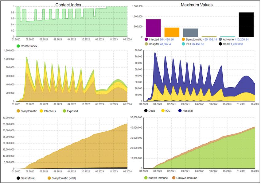
A PREPRINT - A PRIL 14, 2020

1.8M confirmed infections, 115K deaths, and 430K recovered. A major problem is the sudden overload of the health
system with people needing hospitalization, intensive care units (ICU), or ventilation, at the same time. If this happens,
people can not access the help they need and die in an uncontrolled way. In face of that, many countries world-wide
have taken preventive isolation as well as social distancing measures, mainly in order to avoid such an overload and
to flatten and shift the peak stress for the health system, also in order to be able to prepare for the wave of demand.
Another major concern is that personnel in the health system and in other system-relevant sectors must be protected
against infections.
However, this results in a lockdown of public life and causes many other problems, besides the significant restriction
of civil rights it is a major challenge for the economy, income of people, and other negative effects. Therefore, it is
obvious that such a lockdown must be restricted to periods as short as possible and it is a question of utmost relevance
how it is possible to exit from this lockdown such that
       • the peak of health care demand is mitigated so it can be handled by health care resources and
       • contact reduction measures can be relaxed and people can as soon as possible return to normal life.
Undoubtedly, a combination of measures will be required to return safely and in steps to normal life, such as quarantine
of infectious persons, continued control of fatalities and potential repetition of contact reduction measures if they get too
high again, risk-group-adapted partial relaxation of contact reduction, and continued hygienic constraints. App-based
digital contact tracing has also been suggested for epidemic control [2] but is controversial due to privacy issues. Of
specific importance to guide this process are antibody tests in order to know which persons can be assumed to be
immune and, thus, can return to normal life. Such tests are under development but currently no significant capacities do
exist. It is therefore an important question to find
       • requirements for such tests in terms of test capacity, as well as adequate sensitivity and specificity values
       • strategies how these tests can be applied in order to be effective.
Additionally, it must be taken into account that the disease is asymptomatic or shows just mild symptoms in the majority
of cases and can lead to immunity for many (herd immunity). If the lockdown is left too early or in an uncontrolled way,
infections can rebound and successive interventions can become necessary. This should be kept to a minimum.
Currently, an increasing variety of SARS-COV-2 antibody tests is available. From a medical point of view, seroconver-
sion, i.e., positivity of IgM/IgG antibodies can be detected as early as 7-14 days after symptomatic COVID-19 infection
[3]. However, since many patients can still shed oral infectious virus up to 22 days after onset of symptoms or after first
positive COVID-19 PCR test result [3], sole positivity of combined IgM/IgG is not a good indicator for non-infectious
individuals and herd immunity. In this respect, isolated detection of virus-specific IgG should be preferred, because
it has a delayed kinetic in comparison to IgM. Furthermore, with respect to disease modeling and contagiousness a
safety buffer of 14 days added on the date of IgG positivity may be reasonable in order to define a reliable time-point
when a person should be considered recovered and non-infectious. Another important variable of antibody tests is
their specificity and sensitivity. For the reliable calculation of herd immunity a high specificity of an antibody test is
critical and should be >99%. Also, an extremely high sensitivity of the antibody test might be desirable and nice to
have. However, it is not of critical importance, as it can be assumed that most people with a functioning herd immunity
also have sufficiently high antibody levels.
In order to find strategies to defeat the pandemic, epidemiological models are used to support decision making. In
general, there are two main modeling approaches: an aggregate view based on a system of differential equations, also
known as System Dynamics (SD) and an individual-based simulation, also known as Agent-Based Simulation (ABS)
[4]. SD models can describe dynamics on an abstract level, people in certain states are represented by their number and
for the solution just an ordinary system of differential equations needs to be solved. Standard solvers are available, the
size of the system is normally quite small (up to a few ten equations) and a fast, immediate response is possible. In
ABS, each individual is modeled explicitly allowing for stochastic and more detailed behavior, underlying is however
discrete-event simulation causing higher computational costs (note that also repetitions of the simulations are needed
in order to get statistically reliable results). Depending on the goals a suitable modeling approach can be selected. It
is also possible to combine both, as an example of hybrid simulation, which has already been applied successfully in
healthcare simulations [5]. It should be noted that an SD model corresponds to an ABS where all agents are represented
by a Markov chain with the same states as the SD model and the number of agents is taken to infinity [4]. Therefore,
all timing in SD is implicitly exponentially distributed. By splitting the SD variables it is also possible to represent
phase type distributions such as the Erlang distribution which is less variant [6]. This allows for more realism in SD
models. Most models extend well-known SEIR models [7, 8] with the states susceptible, exposed (infected but not yet
infectious), infectious, and recovered. In SD models each equation describes the change of the number of people in
theses states and in ABS each agent has these internal states.

                                                             2
A PREPRINT - A PRIL 14, 2020

A number of simulations with both approaches for the dynamics of COVID-19 have been published recently and are
discussed in Sec. 2. These models describe the dynamics of the disease and the effects of certain interventions. For this
purpose efforts have been undertaken to get important model parameters such as basic reproduction number, incubation
period, case fatality risk, others cannot be accessed and must be estimated, e.g., percentage of contact rate reductions
when interventions are implemented or the percentage of isolated cases. It is however clear that at this stage of the
pandemic there are many uncertainties about these parameters, including the manifestation index, fatality rates as well
as age- and risk-stratified numbers. In this paper we use those models as a reference in order to adequately model the
disease dynamics, adapt them to current data and then add further aspects for investigating exit strategies based on a set
of measures.
The contribution of this paper is to investigate for a country like Germany combinations of measures in order to get an
effective exit strategy and to meet the important goals mentioned above. We will thus investigate the following scenarios:
disease dynamics if no lockdown would have been imposed, an exit of the lockdown without successive measures,
hygienic constraints imposed after lockdown, and repetitive and adaptive but short-term social contact restrictions.
Isolation of infectious people, seasonality of contagiousness, and immunity of a large fraction of the population is also
considered. Antibody tests are used in order to let return people with assumed immunity to public life without contact
reductions. Since such tests are a scarce resource it will not be possible to test all people systematically. Therefore
it will be necessary to develop strategies such that a positive effect can be achieved. One approach is to give people
from risk groups or from system relevant sectors preference, such as health personnel. A second approach is to follow
infection chains and identify people who might have been infected but were asymptomatic (digital contact tracing could
help here). If that is possible, these people will be also tested with preference leading to a higher fraction of people able
to reenter public life. We will first examine these strategies with an extended SD model in order to get main hints. We
will then show an ABS model for a prototypical region with different classes of people. The ABS model will be used in
followup work to check whether properties of testing are sufficient or must be improved. In the SD model all effects are
aggregated in rates for the complete population, whereas in the ABS individual contacts between people in families, at
work, in hospitals, and in leisure are modeled. Thus the ABS allows to draw conclusions also for the availability of
personnel in hospitals and in companies. This also allows for planning over the time during and after lockdown. Both
models have been realized with the simulation framework AnyLogic2 .
The rest of the paper is organized as follows. In Sec. 3 we discuss available data sources, uncertainties within them and
extract our assumptions which we use in both the SD and ABS models. Sec. 4 presents the SD and Sec. 5 the ABS
model. Results are given Sec. 6, conclusions and further work are discussed afterwards.

2       Related work

A number of simulations for the dynamics of COVID-19 have been published recently. SD models for the dynamics
of COVID-19 and the effects of possible interventions are for instance [9], which is accessible online3 , the model of
Robert Koch Institute for Germany [10] which we consider as a reference model for the study presented here. In [11]
an ABS model is presented for studying the dynamics of COVID-19 and possible mitigation and suppression measures
in GB and US, a model representing each inhabitant of Austria4 is based on [12].
A multiple-input deep convolutional neural network model is used in [13] to predict the number of confirmed cases in
China with respect to the number of cases from the past five days. However, no measures such as contact restrictions or
quarantine can be taken into account, but these have a significant impact on the spread of the virus and can lead to a
subexponential growth in the number of cases. Using China as an example, this influence is examined in [14] with an
extended SIR model and in [15] with an extended SEIR model. The agent-based simulation model [16] examines the
influence of interventions on the spread of the virus in Singapore. To predict the local and nationwide spread of the
virus, [17] combines a SEIR model based on differential equations with a metapopulation model based on traffic flows
to model intercity mobility. The influence of traffic restrictions on an international level is examined in [18] with a
combined individual-based subpopulation and a flow-based metapopulation model.
In conjunction with testing, measures to reduce the probability of transmission can be improved. In [19] the influence of
the test coverage with regard to the deceased on the contact rate with an extended SEIR model is examined. According to
the calculations in [20], carrying out mass tests can significantly reduce the economic costs of mitigating the COVID-19
pandemic. For this purpose, the SEIR model is expanded to differentiate between recognized and unrecognized infected

    2
      https://www.anylogic.com/
    3
      covidsim.eu
    4
      http://www.dwh.at/de/neues/wie-man-die-epidemie-berechnen-kann/

                                                             3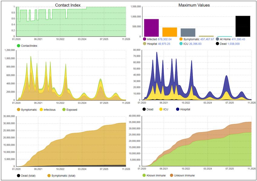
A PREPRINT - A PRIL 14, 2020

people. The influence of such tests can also be tried out using online available SD models5,6 . A particular limiting
factor is the availability of test kits. The pool testing strategy for asymptomatic or mild cases presented in [21] can
reduce test costs and improve the identification of low-risk individuals under the condition, that most tests are negative.
The models without tests for infected persons partially combine the contact reduction to reduce the infection rate with
measures such as isolation or school closure. However, no strategies for adapting these measures are modeled. The
models which consider tests use this extension to continuously adjust the contact rate. Additionally, the study [20] also
switches between phases with a low and phases with a high test rate. All models have in common that they do not take
into account tests for antibodies.

3       Data sources, assumptions, and extended SEIR model

There is a variety of information available about epidemiology of COVID-19, by WHO and in many preprints and
accelerated publications, most of them report insights from Hubai, China. We use the investigations of the Robert
Koch Institute (RKI) which is Germany’s public health institute. It continuously monitors the literature and gives a
characterization7 of facts and numbers for which some evidence is available, last updated on April 10, 2020. It is
clear that at this stage there is much uncertainty in many of those values, but we extract the main findings which are
relevant for modeling. For some required figures RKI does not give characterizations, in these cases we resort to the
assumptions of [10], which are also based on reflections from experienced epidemiologists. Both information sources
are (unfortunately) in German. The presented values are default values which can easily be changed, as will be done in
later experiments.
The manifestation index of showing symptoms when infected is estimated to be within 69% and 86%. However, this
might be larger, some estimations even assume a factor of unknown cases of up to 20. Severity is characterized as mild
or moderate (without or with light pneumonia, 80%), severe (needs hospitalization without ICU, 14%), and critical
(needs ICU 6%). The basic reproduction number R0 is estimated to lie between 2.4 and 3.3, WHO estimates for China
a range between 2 and 2.5 (without interventions). We assume a value of 3 to reflect the recorded cases in Germany. As
in [10] we also allow for seasonal changes according to a sine function. For the incubation period (from infection to
sickness) on the average 5 to 6 days can be assumed (range 1 - 14). For the latency period (from infection to being
infectious) no results are given, we thus assume 3 days. The infection period can be assumed to start 2.5 days before
onset of symptoms, the duration is unclear. Since the severity and duration of cases differ we calculate the infection
period weighted by the number of cases (both symptomatic and asymptomatic), resulting in an average of 12.5 days
including the prodromal period. Symptomatic period in mild or moderate cases is assumed to be 9 days according to
[10], we take the same time for asymptomatic cases. For the time from onset of symptoms to hospitalization an average
of 4 is reported (with an interquartile range IQR of 2 - 7) and from hospitalization to ICU on the average 1 day (IQR
0 - 3). For the hospitalization time of severe cases and for the time in ICU we assume 14 and 10 days respectively
as in [10]. Case fatality rates (CFRs) are counted in different ways and are uncertain, in [10] it is assumed that only
ICU patients die with a percentage of 50%, in the RKI characterization also CFRs of 0.1% (mild) 8.1% (severe), 22%
(critical) are suggested, we count moderate cases to be included into the mild ones. After the disease people have
antibodies and are assumed to be immune. Even though the persistence is unclear, experience from other corona viruses
suggest ca. 3 years, we assume here persistent immunity.
Based on this, a state chart for the progression of the disease from the view of a single person can be defined, it is
shown in Fig. 1 and represents an extended SEIR model. Persons are initially susceptible, then exposed after infection,
after the latency period a person gets infectious and is recovered or dead afterwards. Persons in recovered are assumed
to be immune and cannot be infected again. The state infectious has substates: first there is the state prodromal in
which no or only mild symptoms are shown, afterwards there is a split between asymptomatic and symptomatic cases.
The symptomatic ones are further split into mild, severe, and critical, the last two of them are again subdivided into
sequential states at home, hospitalized, and ICU. We also divide the recovered state into the substates was_asymptomatic
and was_symptomatic, a separation which we need for the antibody tests. At each time instance the state chart is
in exactly one state, for every (sub-)state without substates either a sojourn time distribution (e.g., latency period in
exposed) or an event (e.g., infection by another person in susceptible) for leaving the state must be defined. In case
of more than one outgoing arrow of a state, switching probabilities are required. For instance, persons leaving the
substates of state infectious have different probabilities to get either back to susceptible (if the person is not immune
afterwards, by default this probability is set to zero) or to recovered or dead. All necessary information for such sojourn
times and switching probabilities can be obtained from the data mentioned in the previous paragraph.
    5
      https://exchange.iseesystems.com/public/isee/covid-19-simulator/
    6
      https://forio.com/app/jeroen_struben/corona-virus-covid19-seir-simulator/
    7
      https://www.rki.de/DE/Content/InfAZ/N/Neuartiges_Coronavirus/Steckbrief.html

                                                            4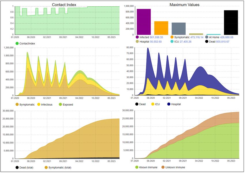
A PREPRINT - A PRIL 14, 2020

                                                          infectious                           recovered (has antibodies)

                                                           asymptomatic                           was_asymptomatic

                                                               symptomatic                         was_symptomatic
                                                         mild: at home

           susceptible   exposed        prodromal      severe: needs hospitalization
                                                         at home       hospitalized
                                                                                                  dead

                                                              critical: needs ICU

                                                       at home     hospitalized       ICU

Figure 1: Extended SEIR model for the progression of the COVID-19 disease from the perspective of a single person

In order to model also aspects like governmental interventions and testing, further attributes are required. Every person
has a social status: normal, reduced, and isolated; initial social status is normal. Considered governmental interventions
are:

       • Reduction: by assigning reduced to many persons, their contact rate is reduced; this models the actual
         lockdown. Without differentiation between population groups, a global percentage of contact reduction can
         be assumed, with 50% as a default value. With differentiation, we can assign different contact reduction
         percentages to, e.g., health personnel, employees in system-relevant sectors, and others. This affects the rate
         of infections significantly. Reduction is applied for persons in every state besides those in which a person is
         isolated or has regained the social status normal because of testing (see below). It is possible to define one
         reduction with its starting time and its duration. Additionally, it is possible to start and stop threshold-based
         reductions: when the CFR gets above or below a definable threshold, respectively.
       • Hygienic constraints: when reduction is taken back, continued hygienic measures are likely to be implemented,
         e.g., mandatory respiratory masks in public life. In the model this causes a contact reduction with a lower
         percentage than in the previous case.
       • Isolation: Persons in substates of symptomatic can be isolated by moving them in specialized isolation wards,
         persons in ICU are isolated anyway. For isolated persons the contact rate is set to zero. Persons in state
         symptomatic staying at home or in hospital get reduced contact rates which can be adjusted (default values are
         zero in both cases). This intervention is assumed to be permanent.

Testing both for COVID-19 and for antibodies (ABs) will be important for an exit of the lockdown. For the time being
we restrict ourselves to AB tests. Every person can be tested (in principle possible in all states, but testing would not
be meaningful in state symptomatic), with either positive or negative outcome. We assume that persons with ABs
are immune and will keep that property indefinitely (could be relaxed later). Therefore, positive ones, regardless in
which state besides symptomatic, can change their social status from reduced to normal. We consider the sensitivity
(by default 95%) of the test, leading to probabilities for true positives and false negatives (negative ones have ABs but
would stay in reduced although not necessary). We assume also a high specifity and ignore false positives (positive ones
without ABs would get normal but can still be infected), because this number is expected to be small. Test capacity is
an important restriction and will be adjusted in the experiments, test duration is assumed to be one day.
A hypothetical unlimited test capacity constitutes a benchmark to investigate the maximum benefit from AB tests.
Since test capacity is however limited, different strategies to allocate tests are conceivable. A first strategy could be to
give preference to persons in state was_symptomatic and allocate possible leftover capacity to all others randomly. A
drawback of this strategy is that most test capacity would be used for symptomatic recovered, who will probably have

                                                              5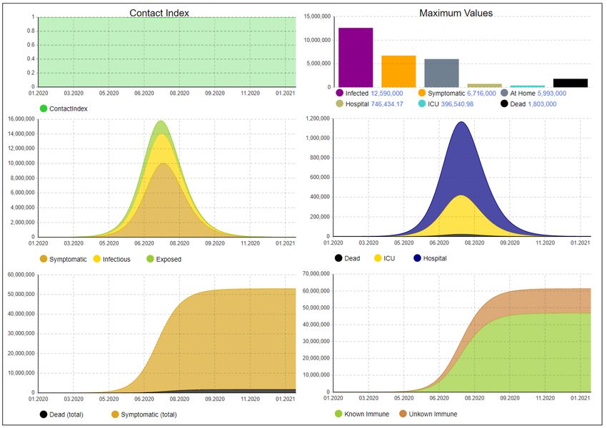
A PREPRINT - A PRIL 14, 2020

                                                                                 FAS FMS FSsS FICUS

                                                                        A
                                                                                                                 FA                                 FAu
                                                           FPA     Asymptoma
                                                                       tic
                                                                                                                                        wasAsymp_
                                                                                                                                        AB_unkown
                                                                                                                                                       wasAsymp_
                                                                                                                                                        AB_kown

                                                                                                                                          Au              Ak

                       FS                 FE      P                                                                                 FR              FSu
         Susceptible         Exposed           Prodromal
                                                                  Mild_at_ho                                FM                Regen‐     wasSymp_AB   wasSymp_AB

             S                  E                           FPM       me
                                                                            M
                                                                                             FMD
                                                                                                                              eration     _unkown       _kown

                                                                                                               FSs              R            Su           Sk
                                                                  Severe_at_           Severe_hos
                                                                                                                           FICUSu
                                           FI              FPSm                  FSm
                                                                    home                  pital
                            Infections_
                              Outside
                                                                     Sm                    Ss         FSsD                                  D‘
                               IO                                 Critical_at_         Critical_hos

                                                                                 FCm                                       FICUD
                                                                                                            Critical_ICU                   Dead
                                                           FPCm      home

                                                                    Cm
                                                                                           pital

                                                                                          Cs          FCs     ICU

                                                      Figure 2: SD model for the COVID-19 disease

ABs. An effective strategy would be to use tests mainly for persons in state was_symptomatic, because this can be many
and they can change their social status from reduced to normal. Given it is possible to identify them, they should get a
preference. Such an identification is to a certain degree possible by following infection chains and could be even more
accurate by digital tracing. In order to represent such strategies in a flexible way, we will use percental weights for
persons in the different states. E.g., a complete random strategy would allocate the same weight to all states, whereas a
strategy giving preference to persons in was_symptomatic, leaving no capacity for persons in was_symptomatic, and
distributing smaller capacities to others without symptoms could be: was_asymptomatic → 40%, was_symptomatic →
0%, asymptomatic → 20%, prodromal → 15%, exposed → 15%, susceptible → 10%. The probability of a person to
get tested is proportional to the number of persons in the same state and the weight.

4   System dynamics (SD) model

Based on the extended SEIR model of Sec. 3 an SD model is derived and shown in Fig. 2. SD models consist of stocks
(continuous variables representing the number of persons in this state) and flows between them (associated with rates
between the stocks). It is possible to derive flow rates from the sojourn times and switching probabilities presented in
Sec. 3. Each colored rectangle corresponds to a stock with a name derived from the state chart in Fig. 1, each arrow
corresponds to a flow, shorter names are also given for the underlying mathematical equations. The equations define the
model precisely and are given with all parameters in Appendix A.
Note that the two states was_asymptomatic and was_symptomatic are split into 4 stocks: wasAsymp_AB_unknown,
wasAsymp_AB_known, wasSymp_AB_unknown, and wasSymp_AB_known, in order to separate between cases where
recovered persons have ABs but this is not known vs. cases in which it is known because of AB tests. In case of
asymptomatic and recovered persons this is completely unknown and in case of symptomatic and recovered persons
it can be supposed that they have ABs but without certainty. There is also an additional stock to represent infections
coming from outside. The stock Regeneration is only implemented to account for the fact that people are considered
as recovered with a delay. It is used since patients after being sick cannot directly participate in public life and its
duration is set to 5 days to reflect values in Germany. However, it can as well be omitted, since it only delays statistics
for recovered people. Flow FAu corresponds to true positive AB tests of recovered with ABs who were asymptomatic
whereas flow FSu corresponds to those who were symptomatic. For the corresponding flow rates factors need to be
computed consisting of the sensitivity, the proportion of the outgoing stock, and the weight mentioned in Sec. 3. These
factors need to be normalized and multiplied with the available test rate, for details please check the Appendix.
There are several possible paths to extend the SD model. First, PCR tests could also be integrated. Second, to make
timing more realistic, the implicit exponential distribution could be replaced by the Erlang distribution by splitting
stocks into sequences. Third, to allow for sub-populations inside the model, the stocks could also be split. All extensions
would make modeling more complicated but would not be challenging for the numerical solution.

                                                                                  6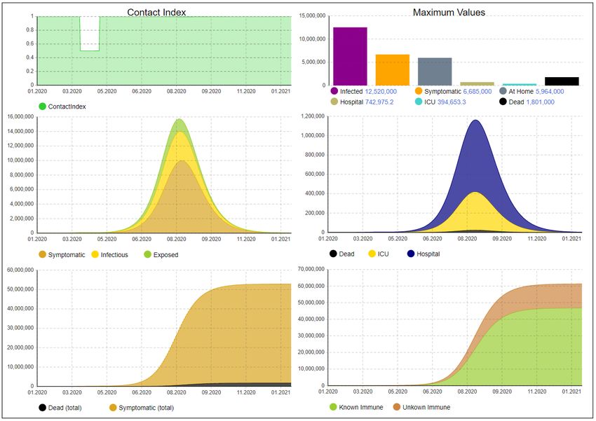
A PREPRINT - A PRIL 14, 2020

                           Figure 3: Screenshot of the ABS model for the COVID-19 disease

5   Agent-Based Simulation (ABS) Model

This modeling approach allows to implement a more realistic simulation. In this case each person is represented by
an agent which has individual attributes and follows one or more behavior models. In our ABS model agents are
combined in different groups which are related to the locations where they can meet and infect each other considering
group-related probabilities. Those are home/family, leisure (including activities like shopping, sports, etc.), being at
hospital, and work. Depending on the current contact reduction level they can change their states. In case of isolation
the agent remains at the quarantine location without changing its state. In order to evaluate a profession-based exit
from the lockdown, different types of workers are considered, namely, system-relevant, not system-relevant, hospital
staff, and others. In particular, the latter represent the non-working population including children and retired persons.
Each worker is linked to a different sized company with other workers in order to avoid direct infections between the
whole working population. The total number of companies is an input parameter that allows to generate large and
small companies. Similarly, different sized households are built and persons are assigned to one certain home group.
Healthcare workers can meet their colleagues, but also patients who are potentially infected. The infection probability
between patients and healthcare personnel can be pre-configured separately from the infection between colleagues.
A further state chart represents the disease states of agents. Beginning by susceptibles, the statechart shows a behavior
which is very close to the conceptual SEIR model of Sec. 3. By configuring the daily capacity for antibody tests, they
can be applied following one of the defined strategies in Sec. 3. As the ABS model differentiates between working
groups and other individual attributes, an even more precise testing strategy can be evaluated. For example, hospital
staff and system-relevant workers can be tested with a higher priority. Input configuration allows to preset a sensitivity
and a specificity value for the test. For a more precise analysis, it is even possible to consider different error probabilities
for agents that are affected and have not been recovered yet. Fig. 3 shows a screenshot of the model with 20.000 agents,
the agents are shown as icons in their environments, colors represent their states. The model can deal with several ten
thousand agents easily and is ready to study effects in a region, but differentiated for the agent groups. It is for instance
possible to derive figures of health personnel with ABs. It will also easily be possible to include other important aspects
into the ABS model: age-dependent severity and CFRs, controlled change of social status (from reduced to normal)
depending on vulnerability (e.g., elderly and other risk groups), viral load at infections (can influence severity), etc.
Resource-based analysis can show, if enough beds, hospital staff, or system-relevant workers are available when the
pandemic gets more severe. It would also be interesting to model regional clusters with ABS and connect them via
continuous flows or to provide an SD environment with the general disease dynamics for the ABS model of a region,
similar as in [5].

                                                               7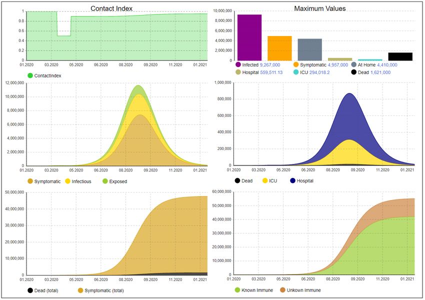
A PREPRINT - A PRIL 14, 2020
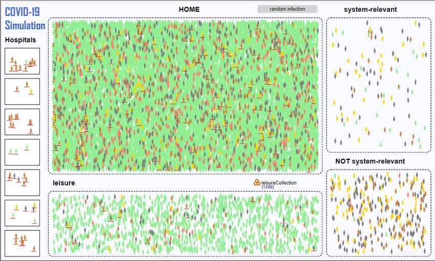
Figure 4: Disease dynamics until April 19
6 Results
We now present the results obtained with the SD model. We calibrated the model to reflect the real progress of the
disease in Germany while staying as close as possible to the RKI values. Fig. 4 shows the model results with this
calibration, the parameters are provided in the Appendix. The left upper curve show a contact index which we have
defined in order to illustrate the overall effect of the interventions on the social contact abilities of people. It gives the
contact abilities averaged over all people who are not symptomatic: if there would be no intervention, all people would
have full contact abilities and the index would be equal to one. Maximum values of critical figures over the simulated
time period such as the number of hospitalized or the number of patients needing ICU are shown in the right upper bar
chart. In the middle row the progress of relevant figures such as number of symptomatic, other infected and exposed
persons is shown on the left and daily deaths, ICU, and hospitalization needs on the right. The lower row shows on
the left cumulated numbers of deaths and people who had been symptomatic. On the right, the grow of the number of
persons is shown for which immunity can be assumed (if this number reaches ca. 60%, herd immunity can be assumed).
The curve is split into known and unknown ones. The unknown ones are constituted in principle by those who had been
symptomatic and are recovered or an AB test has been performed for them. In Fig. 4 no such AB tests are considered,
but below we will investigate effects of AB tests.
Compared to RKI, we assume a higher ICU capacity due to the report of hospital utilization (ca. 27K ICU places)8 .
The reproduction number is set to 3, meaning that on average, one infected person can spread the virus to three other
persons. However, if the infected persons get symptomatic and stay at home, their contact rate is halved such that they
only can infect half the number of persons. If they are isolated in a hospital, we assume that they infect on average one
additional person, for example in their family, before they are isolated. We also slightly increased the number of people
that require treatment in hospitals and ICUs to model the number of confirmed cases in Germany. The evolution of the
virus in Germany has three distinctive time instants: 1) it started on January 22, 2) the majority of interventions have
been introduced after March 22, and 3) the latest available data time when this paper has been written. We reflect the
8
https://www.intensivregister.de/#/intensivregister
8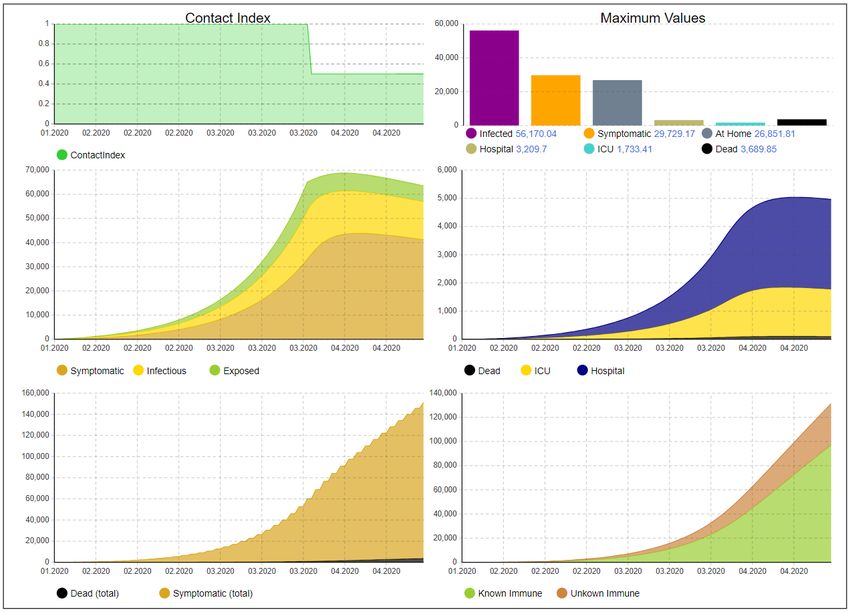
A PREPRINT - A PRIL 14, 2020

                                 Figure 5: Disease dynamics without any intervention

real number of infections and deaths according to the statistics provided by Johns Hopkins University9 . The model tries
to match the situation at all three times instants as close as possible. However, it is clear that we can only model an
idealized behavior. We match the cumulative number of infections, deaths, and recoveries, as well as the ICU utilization
with the first infection on January 22 and the interventions beginning on March 22.
Using these adjusted parameters, how would the disease have evolved, if no interventions would have been imposed?
Fig. 5 shows the dynamics under this assumption. As can be seen, the ICU utilization is highly exceeded (ca. 400K at its
peak). Thus, this scenario would lead to a fairly higher number of deaths than shown in the figure because of significant
overload of ICU capacities since we do not model maximum capacities but only reflect the required numbers. We now
investigate the effect of these initial interventions between March 22 and April 19, without successive interventions,
as illustrated in Fig. 6. We can see that the peak is only shifted to the right but not significantly reduced. This is a
strong indication that the interventions cannot be released without substitution. Fig. 7 shows a scenario where the
population is required to keep hygienic constraints (e.g., by using mouthpieces). It can be seen that the curve is clearly
flattened, but the ICU utilization is still significantly too high (ca. 300K). The contact index shows the restrictions
for the population by about 10% due to these hygienic measures but also that they can be reduced over time due to
increasing immunization.
We use these insights to find an exit strategy which does not overload the health system, specifically ICU capacity.
Contact reductions, as in the first lockdown, are triggered, if the current ICU occupation exceeds a certain threshold.
Such additional adaptive restrictions periods should be short-term and can be released when the number falls below the
threshold, however, in order to avoid oscillations, a minimum of two weeks for such reductions is assumed. This can
easily be changed to other values or other indicators such as the number of deaths per day. This behavior can be directly
transferred to reality by monitoring the utilization of the available ICU capacity and apply interventions if this number
exceeds or falls below a certain threshold. Due to the delay when interventions affect the number of infections, we
need to apply a threshold of 18.5K to ensure that the ICU capacity is not exceeded. The progression of the disease
and the necessary interventions are illustrated in Fig. 8. As we can see, the model predicts that 9 additional intervals
with contact restrictions would be necessary. The last intervention would end in March 2023 and also all hygienic

   9
       https://coronavirus.jhu.edu/map.html

                                                            9
A PREPRINT - A PRIL 14, 2020
Figure 6: Disease dynamics without further interventions after April 19
Figure 7: Disease dynamics with hygienic constraints but no other interventions after April 19
10A PREPRINT - A PRIL 14, 2020
Figure 8: Disease dynamics with hygienic constraints and adaptive contact restrictions if ICU occupation exceeds a
threshold
measures could be dropped in 2023. Of course, the model can be adapted if new information about the disease is known,
e.g., on seasonality. With an increasing number of recovered people after the infection, less people would be affected
by interventions as reflected by the contact index. However, since this is a long period where interventions would be
needed, we want to reduce the number of affected people as far as possible to reduce the economic and social impact
but still introduce no additional risks for the population.
To achieve this, we now consider a scenario with AB tests, which we assume to start already after April 19. It is of
course not yet realistic to have a significant capacity for AB tests in such a short term, but later in this year it could be
accomplished if serious efforts are expended. We assume the same combination of interventions as in the last scenario
(adaptive contact restrictions after the lockdown, hygienic measures). First of all, if test capacity would be unlimited,
all unknown immunes would become known immunes, thus the orange stripe in Fig. 8 shows the maximum potential of
AB tests which is 6.2M for this scenario. We now assume a test strategy in which preference is given to asymptomatic
recovered persons and persons who had been symptomatic are not tested. Assuming that the asymptomatic recovered
ones can be identified to some extend, we assign weights: was_asymptomatic → 40%, was_symptomatic → 0%,
asymptomatic → 20%, Prodromal → 15%, Exposed → 15%, Susceptible → 10%.
Based on these assumptions the test capacity has been varied and the effects have been observed. It turns out that up
to a capacity of 100K tests per day the number of people who can be excluded from contact reductions is increased
significantly, afterwards less significant increase can be noticed. Even though requiring a high number of tests this does
not seem to be completely out of scope if testing infrastructures can be scaled up. The effect with a capacity of 100K is
illustrated in Fig. 9. As can be seen, up to 5.4M people can be excluded additionally from interventions with these tests
(compared to 25.4M without tests). With a lower number of tests, e.g., 50K per day, we would still be able to exclude
4.4M people. If we apply these tests with preference to system-relevant groups, we can significantly improve public life
(as a reference, ca. 1M nurses and related jobs are registered in Germany10 ). If we assume a more pessimistic value
for the test sensitivity (75%), the effects are marginally reduced. With 50K tests per day, we would still be able to
exclude 4M additional people. However, the effectiveness of AB testing significantly depends on the identification
of asymptomatic recovered persons. If we assume that they cannot be identified (i.e., uniform weights for all stocks
10
https://www.bundesgesundheitsministerium.de/themen/pflege/pflegekraefte/beschaeftigte.html
11A PREPRINT - A PRIL 14, 2020
Figure 9: Disease dynamics with hygienic constraints and adaptive contact restrictions if ICU occupation exceeds a
threshold and application of antibody tests
besides was_symptomatic which gets 0%), the number of additionally detected people with antibodies for 50K tests per
day reduces to 2M. To achieve the similar effect as in Fig. 9 before, the number of tests need to be increased even up to
250K. This shows that tracking might be a valuable tool for future exit strategies.
The importance of AB tests would be even greater if the disease spreads more drastically, e.g., due to non-optimal
interventions. This in turn would lead to more infections and in turn to more asymptomatic recovered and thus increase
the likelihood of finding people with antibodies, making the tests more effective and excluding more people from
interventions. However, we have not added figures for these scenarios because the ICU capacities would be exceeded
and the number of deaths would increase significantly, as discussed in the previous scenarios.
Fig. 10 and 11 demonstrate how the virus spreading would be affected if a seasonality factor is in place, meaning that
the virus spreads less in summer and more in winter months, or if a significant portion of the population is immune to
the virus. The seasonality is modeled as sine curve, as also explained in the Appendix. The figures show the dynamics
with no antibody testing in place, the number of immune people and thus the contact index could be improved with the
previously described measure by the number of unknown immune people tracked by the bottom right curve. We omitted
the graphics for space reasons but the number of additionally identified immune people behaves nearly identically
as with the effect shown in Fig. 8 and 9. As we can see, the dynamics of the virus are similar, the disease will still
spread fast after April 19 and would exceed ICU capacities. The main difference is the number of interventions that
will be required, which reduces from 9 to 6 (for seasonality) or 5 (for initially immune people). If an initial immunity
of one third of the population is assumed, the last intervention is already in November 2021. To optimally propose
interventions, our model can thus be adapted when more information for this behavior is known. However, currently,
we assume the worst-case behavior without seasonality and no initial immunization.
7 Conclusions
We have presented a system dynamics (SD) and an agent-based simulation (ABS) model for COVID-19. The models can
represent the disease dynamics on different abstraction levels and can also be used to study governmental interventions
12A PREPRINT - A PRIL 14, 2020
Figure 10: Disease dynamics if the virus is more infectious during winter months, less in summer (R0 fluctuates
between 3.1 and 2.1 with sine curve)
Figure 11: Disease dynamics if one third of the population is generally immune to the virus
13A PREPRINT - A PRIL 14, 2020
and the effects of antibody tests. Starting from parameters suggested by other COVID-19 models recently presented we
adapted the parameters to published data for Germany and investigated derived scenarios from that. Based on these
assumptions about parameters and the SD model, which is of course a simplified abstraction of reality, we could gain
the following key insights for a country like Germany:
• Without enacting interventions such as the lockdown in March 2020, the disease would cause significant
overload of the health system with many deaths expected. This is in agreement with the findings of other
COVID-19 models.
• If the lockdown would just be released after 4 weeks in April and a return takes place to the status before
lockdown, the disease can be expected to rebound just with a slight delay corresponding to the time of the
lockdown, meaning that a little time has been gained in order to prepare the health system better but with the
same potentially large number of deaths.
• If hygienic measures are put in place after lockdown, a slight mitigation can be expected but this alone would
not be sufficient to defeat the disease.
• This however can be achieved with repetitive short term contact reductions similar to the current lockdown;
such reductions can be triggered adaptively, if relevant figures (such as death rates, need for ICU, etc.) exceed
a threshold. With additional hygienic measures the situation can be enhanced further. However, we can expect
that this situation (repetitive short term lockdowns and hygienic measures) needs to be in place for the next
two or three years until herd immunity can be obtained (if vaccination is not available before).
• The effects of antibody tests would add significant benefit in order to exclude people with antibodies from the
contact reductions. Results show that already a moderate infrastructure for antibody tests (50K per day for
Germany) would lead to significant improvements bringing ca. 4.4M people back to public life compared to
scenarios without such possibilities. With a higher test capacity (e.g., 100K) this number could be pushed to
more than 5.4M. Digital tracing could improve the efficiency of AB tests. If immunity will be lost after some
time, AB testing would become even more important.
• Seasonality of the disease and general immunization would lead to significant mitigation effects while still
requiring the described mechanisms.
• A contact index to condense the social contact abilities for all people has been defined, it can illustrate well the
effect of the combination of all measures.
Both models can be extended in several ways in order to study the interaction between further effects of the disease and
more sophisticated exit strategies, such as benefits from PCR tests as well, age- and risk-dependent severity and fatality
rates, more detailed consideration of infectiousness during the phases of illness, influence of viral load on severity,
differentiation of measures for vulnerable groups of people, etc. One promising approach for this is to combine both
models to a hybrid simulation model as in [5] in which both general trends and details for regions, different groups of
persons, and more exit strategies can be studied. The models can be adapted to latest data as the pandemic is progressing
in order to adapt interventions accordingly. The integration of digital tracing for epidemic control (alerting people in
case of previous contacts with people who have been infected) [2] into the set of measures is also promising and can be
investigated with the presented models.
14A PREPRINT - A PRIL 14, 2020
A SD model details
We provide all initial stock values, equations, and parameters of the SD model.
A.1 Initial stock values
All stocks besides the following are initially set to zero:
• S = (1 − pinit_immune ) ∗ N − IF
• P = IF
• Ak = pinit_immune ∗ N
A.2 Differential equations of the output flows
Flow Output of Formula n
S
FS = N −IO−D ∗ fc ∗ (A + P ) ∗ (1 − pinterven )
Susceptible (note that o (1)
FS + Hos ∗ (1 − piso_hos ) + Hom ∗ (1 − piso_hom )
IO ≤ 0 for t ≥ 0)
R(t)
basic contact rate: fc = p
P rodRed ∗Dp +(Di −Dp )
number of people in hospital: Hom = M + Sm + Cm − IsoHom
number of people at home: Hos = Ss + Cs − IsoHos
Note: Infections from outside are treated as normal Prodromals
E
FE Exposed FE = (2)
De
FIO Infections_Outside FIO = Iout (3)
P
FP A Prodromal to Asymptomatic FP A = (1 − pmani ) ∗ (4)
Dp
P
FP M Prodromal to Mild at home FP M = pmani ∗ (1 − psick_hosp ) ∗ (5)
Dp
P
FP Sm Prodromal to Severe at home FP Sm = psev ∗ (6)
Dp
Prodromal to Critical at P
FP Cm FP Cm = pcrit ∗ (7)
home Dp
Asymptomatic to A
FA FA = pimmun ∗ (8)
wasAsymp_AB_unkown Da
Mild_at_home to M
FM FM = pimmun ∗ (1 − pdeathM ild ) ∗ (9)
Regeneration Dm
15A PREPRINT - A PRIL 14, 2020
Flow Output of Formula
Severe_at_home to Sm
FSm FSm = (10)
Severe_hospital DSymT oHos
Severe_hospital to Ss
FSs FSs = pimmun ∗ (1 − pdeathSev ) ∗ (11)
Regeneration Dsev_hos
Critical_at_home to Cm
FCm FCm = (12)
Critical_hospital DSymT oHos
Critical_hospital to Cs
FCs FCs = (13)
Critical_ICU DHosT oICU
Critical_ICU to ICU
FICU Su FICU Su = pimmun ∗ (1 − pdeathICU ) ∗ (14)
Regeneration DICU
ICU
FICU D Critical_ICU to Dead FICU D = pdeathICU ∗ (15)
DICU
Ss
FSsD Severe_hospital to Dead FSsD = pdeathSev ∗ (16)
Dsev_hos
M
FM D Mild_at_home to Dead FM D = pdeathM ild ∗ (17)
Dm
Asymptomatic to A
FAS FAS = (1 − pimmun ) ∗ (18)
Susceptible Da
Mild_at_home to M
FM S FM S = (1 − pimmun ) ∗ (1 − pdeathM ild ) ∗ (19)
Susceptible Dm
Severe_hospital to Ss
FSsS FSsS = (1 − pimmun ) ∗ (1 − pdeathSev ) ∗ (20)
Susceptible Dsev_hos
ICU
FICU S Critical_ICU to Susceptible FICU S = (1 − pimmun ) ∗ (1 − pdeath ) ∗ (21)
DICU
Regeneration to R
FR FR = (22)
wasSymp_AB_unkown Dr
Su pAB_wasSym
stock size and test ratio weighting: wSu = Ttot ∗ pAB_tot
wasSymp_AB_unkown to 1
FSu FSu = psens ∗ wSu ∗ ∗ TAB (23)
wasSymp_AB_kown
wtot
Au pAB_wasAsym
stock size and test ratio weighting: wAu = Ttot ∗ pAB_tot
wasAsymp_AB_unkown to 1
FAu FAu = psens ∗ wAu ∗ ∗ TAB (24)
wasAsymp_AB_kown
wtot
16A PREPRINT - A PRIL 14, 2020
A.3 Parameters
Parameter Default Value Description
N 83,000,000 total population (initally)
pinit_immune 0 percentage of initially immune persons
IF 1 number of initially infectious persons
percentage of contagiousness of prodromal vs. later
pP rodRed 50%
infectious states
current reproduction number, average R0 average,
Rvar amplitude
R(t) R0 = 3, Rvar = 0 R(t) = R0 − sin(0.0172 ∗ (t − c)) ∗ Rvar (25)
with c being the shift in time dependent on the
simulation start date.
infection period (depends on duration of infectious
Di calculated: 12.5 days
stages, only used for FS )
De 2 days latency period
Dp 3 days prodromal period
Dm 9 days symptomatic period in mild cases
Da 9 days asymptomatic period
DSymT oHos 4 days from onset of symptoms to hospitalization
Dsev_hos 14 days hospitalization time in severe cases
DHosT oICU 1 day from hospitalization to ICU
DICU 10 days time in ICU
duration that the state recovered is delayed after being
Dr 5 days
ill
percentage of reduction during governmental contact
pinterven 50%
reduction intervention
pmani 80% percentage of infections that show symptoms
psev psev = pmani ∗ psick_hosp percentage of infections that are severe
pcrit psev = pmani ∗ psick_hosp ∗ phosp_ICU percentage of symptomatic persons that are critical
psick_hosp 8% percentage of symptomatic persons that need hospital
phosp_ICU 75% percentage of persons in hospital that need ICU
pimmun 100% percentage of persons that are immune after infection
pdeathICU 50% CFR in critical cases
pdeathSev 8.1% CFR in severe cases
pdeathM ild 1% CFR in mild cases
TAB 25,000 daily capacity of AB tests
psens 95% sensitivity of AB tests
pAB_wasSym 0.05 AB test weight for the Au stock
pAB_wasAsym 0.3 AB test weight for the Su stock
IsoHom IsoHom = (M + Cm + Sm) ∗ piso_ward number of persons isolated completely at home
number of persons isolated completely while in
IsoHos IsoHos = (Cs + Ss) ∗ piso_ward
hospital
percentage of people that can be isolated completely
piso_ward 0%
(using isolation wards)
piso_red 100% percentage of contact reduction in isolation
wtot wtot = wAu + wSu + wS + wE + wP + wA normalization factor for test weighting
Ttot Ttot = S + E + P + A + Au + Su total people that can be tested
daily infection rate from outside, first value if no
Iout 70 or 1
intervention is active, else second value
threshold values for which interventions start and end
T _max & T _min 18500 & 9500 (can be applied to number of patients in ICU, deaths
per day, infections per day, and so on)
percentage that optional hygienic measures after the
phyg 10%
initial intervention reduce the spreading of the virus
17A PREPRINT - A PRIL 14, 2020
References
[1] Ensheng Dong, Hongru Du, and Lauren Gardner. An interactive web-based dashboard to track COVID-19 in
real time. The Lancet, Infectious Diseases, February 19 2020, https://doi.org/10.1016/S1473-3099(20)
30120-1.
[2] Luca Ferretti et al. Quantifying SARS-CoV-2 transmission suggests epidemic control with digital contact tracing.
Science, 2020, https://doi.org/10.1126/science.abb6936.
[3] Wölfel et al. Virological assessment of hospitalized patients with COVID-2019. Nature, 2020, https://doi.
org/10.1038/s41586-020-2196-x.
[4] Hazhir Rahmandad and John Sterman. Comparing agent-based and differential equation models. INFORMS
Management Science, 54(5):998–1014, 2008, https://doi.org/10.1287/mnsc.1070.0787.
[5] Anatoli Djanatliev and Reinhard German. Prospective Healthcare Decision-Making by Combined System
Dynamics, Discrete-Event and Agent-Based Simulation. In Proceedings of the 2013 Winter Simulation Conference,
pages 270–281. IEEE Press, 2013, https://doi.org/10.1109/WSC.2013.6721426.
[6] Olga Krylova and David J D Earn. Effects of the infectious period distribution on predicted transitions in
childhood disease dynamics. Journal of the Royal Society, Interface, 10(84):998–1014, 2013, https://doi.
org/10.1098/rsif.2013.0098.
[7] William Ogilvy Kermack and A. G. McKendrick. A contribution to the mathematical theory of epidemics. Proc.
of the Royal Society of London Series A, 115:700–721, 2013, https://doi.org/10.1098/rspa.1927.0118.
[8] Herbert W. Hethcote. The mathematics of infectious diseases. SIAM REVIEW Society for Industrial and Applied
Mathematics, 42(4):599–653, 2000.
[9] Nick Wilson, Lucy Telfar Barnard, Amanda Kvalsig, Ayesha Verrall, Michael G Baker, and Markus Schwehm.
Modelling the potential health impact of the COVID-19 pandemic on a hypothetical European country. medRxiv,
2020, https://doi.org/10.1101/2020.03.20.20039776.
[10] Matthias an der Heiden and Udo Buchholz. Modellierung von Beispielszenarien der SARS-CoV-2-Epidemie 2020
in Deutschland. 2020, https://doi.org/10.25646/6571.2.
[11] Neil M Ferguson et al. Impact of non-pharmaceutical interventions (NPIs) to reduce COVID-19 mortality and
healthcare demand. 2020, https://doi.org/10.25561/77482.
[12] C. Urach K. Bicher and N. Popper. GEPOC ABM: A generic agent-based population model for Austria. In
Proceedings of the 2018 Winter Simulation Conference, pages 2656–2667, Gothenburg, Sweden, 2018.
[13] Chiou-Jye Huang, Yung-Hsiang Chen, Yuxuan Ma, and Ping-Huan Kuo. Multiple-input deep convolutional
neural network model for COVID-19 forecasting in China. 2020, https://doi.org/10.1101/2020.03.23.
20041608.
[14] Benjamin F Maier and Dirk Brockmann. Effective containment explains subexponential growth in recent confirmed
covid-19 cases in China. Science, 2020, https://doi.org/10.1126/science.abb4557.
[15] Qianying Lin, Shi Zhao, Daozhou Gao, Yijun Lou, Shu Yang, Salihu S. Musa, Maggie H. Wang, Yongli Cai,
Weiming Wang, Lin Yang, and Daihai He. A conceptual model for the coronavirus disease 2019 (COVID-19)
outbreak in Wuhan, China with individual reaction and governmental action. International Journal of Infectious
Diseases, 2020, https://doi.org/10.1016/j.ijid.2020.02.058.
[16] Joel R Koo, Alex R Cook, Minah Park, Yinxiaohe Sun, Haoyang Sun, Jue Tao Lim, Clarence Tam, and Borame L
Dickens. Interventions to mitigate early spread of SARS-CoV-2 in Singapore: a modelling study. The Lancet
Infectious Diseases, 2020, https://doi.org/10.1016/s1473-3099(20)30162-6.
[17] Joseph T Wu, Kathy Leung, and Gabriel M Leung. Nowcasting and forecasting the potential domestic and
international spread of the 2019-nCoV outbreak originating in Wuhan, China: a modelling study. The Lancet,
395(10225):689–697, 2020, https://doi.org/10.1016/s0140-6736(20)30260-9.
[18] Matteo Chinazzi, Jessica T Davis, Marco Ajelli, Corrado Gioannini, Maria Litvinova, Stefano Merler, Ana Pastore
y Piontti, Kunpeng Mu, Luca Rossi, Kaiyuan Sun, et al. The effect of travel restrictions on the spread of the 2019
novel coronavirus (COVID-19) outbreak. Science, 2020, https://doi.org/10.1126/science.aba9757.
[19] Navid Ghaffarzadegan and Hazhir Rahmandad. Simulation-based estimation of the spread of COVID-19 in Iran.
2020, https://doi.org/10.1101/2020.03.22.20040956.
[20] Patrick Jenny, David F Jenny, Hossein Gorji, Markus Arnoldini, and Wolf-Dietrich Hardt. Dynamic modeling
to identify mitigation strategies for Covid-19 pandemic. 2020, https://doi.org/10.1101/2020.03.27.
20045237.
18A PREPRINT - A PRIL 14, 2020
[21] Nasa Sinnott-Armstrong, Daniel Klein, and Brendan Hickey. Evaluation of group testing for SARS-CoV-2 RNA.
2020, https://doi.org/10.1101/2020.03.27.20043968.
19You can also read