Prediction of gas velocity in two phase flow using developed fuzzy logic system with differential evolution algorithm
←
→
Page content transcription
If your browser does not render page correctly, please read the page content below
www.nature.com/scientificreports
OPEN Prediction of gas velocity
in two‑phase flow using developed
fuzzy logic system with differential
evolution algorithm
Meisam Babanezhad1,2,3, Samyar Zabihi4, Iman Behroyan5,6, Ali Taghvaie Nakhjiri7,
Azam Marjani8,9* & Saeed Shirazian10
In this investigation, differential evolution (DE) algorithm with the fuzzy inference system (FIS) are
combined and the DE algorithm is employed in FIS training process. Considered data in this study were
extracted from simulation of a 2D two-phase reactor in which gas was sparged from bottom of reactor,
and the injected gas velocities were between 0.05 to 0.11 m/s. After doing a couple of training by
making some changes in DE parameters and FIS parameters, the greatest percentage of FIS capacity
was achieved. By applying the optimized model, the gas phase velocity in x direction inside the reactor
was predicted when the injected gas velocity was 0.08 m/s.
A major role is played by liquid/gas systems in a variety of chemical engineering sectors. One of the most
renowned technical equipment is bubble columns reactors which are usually used for contacting between two
gas and liquid phases. Bubble columns are normally applied for slow kinetic reactions like oxidation, alkyla-
tion, hydrogenation, hydroformylation, decarbonization, Fischer–Tropsh synthesis, desulfurization, and
fermentation1,2.
Wastewater treatment sites, producers of organic acids, yeasts, and cell cultures utilize these reactors in their
processing sites3. The form and shape of these columns are simple, with no moving element. In addition, these
reactors are featured with economical operation costs, easy maintenance, and desirable mass/heat transfer flux. As
the disadvantages, complicated hydrodynamics deeply depend on the geometry and flow velocities. In addition,
local/global parameters (flow pattern, phase velocities, gas phase hold-up, turbulence, and bubble size) have a
direct and complicated effect on the design variables.
Bubble column (BC) reactors are usually utilized in industrial work like heterogeneous churn turbulent flow
pattern4. Thereby, it is imperative to examine such columns under such operational circumstances for better
performance and optimization. There have been many empirical correlations developed to design such systems.
Such correlations normally possess a limited validity domain as to operating conditions, geometries, or physical
properties. There is a need to develop new computation models to simulate bubble column reactors with a wider
validity range compatible with both homogeneous/heterogeneous flow patterns.
For years, the only way of scaling up bubble columns was through macroscopic equations to elaborate on
hydrodynamics of system5,6. Currently, however, computational fluid dynamics (CFD) technique is employed
ows7 and eliminate the limits of the con-
as a reliable procedure to find local/global properties through bubbly fl
ventional scale-up method through costly experimental measurements.
To function effectively, bubble column reactors need efficacious liquid—gas phases mass, momentum, and
energy transfers. While bubble column reactors have simple design, the modelling is not easy. Operational and
1
Institute of Research and Development, Duy Tan University, Da Nang 550000, Vietnam. 2Faculty of
Electrical‑Electronic Engineering, Duy Tan University, Da Nang 550000, Vietnam. 3Department of Artificial
Intelligence, Shunderman Industrial Strategy Co., Tehran, Iran. 4Department of Process Engineering, Research
and Development Department, Shazand-Arak Oil Refinery Company, Arak, Iran. 5Faculty of Mechanical and
Energy Engineering, Shahid Beheshti University, Tehran, Iran. 6Department of Computational Fluid Dynamics,
Shunderman Industrial Strategy Co., Tehran, Iran. 7Department of Petroleum and Chemical Engineering, Science
and Research Branch, Islamic Azad University, Tehran, Iran. 8Department for Management of Science and
Technology Development, Ton Duc Thang University, Ho Chi Minh City, Viet Nam. 9Faculty of Applied Sciences, Ton
Duc Thang University, Ho Chi Minh City, Viet Nam. 10Laboratory of Computational Modeling of Drugs, South Ural
State University, 76 Lenin Prospekt, Chelyabinsk 454080, Russia. *email: azam.marjani@tdtu.edu.vn
Scientific Reports | (2021) 11:2380 | https://doi.org/10.1038/s41598-021-81957-3 1
Vol.:(0123456789)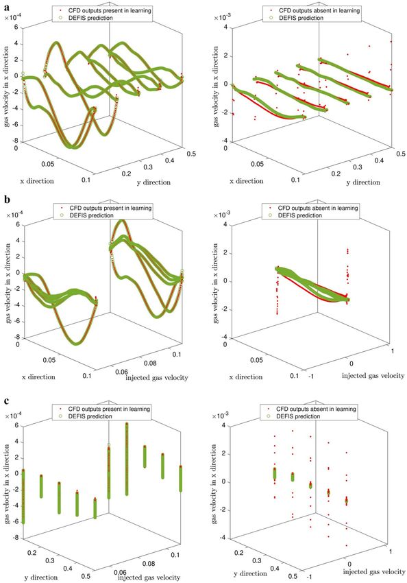
www.nature.com/scientificreports/
design parameters of the column, which are related to each other in a complicated manner, dictate phase velocity,
gas volume fractions, bubble size, flow regime, and turbulence. There are unmet needs with models to simulate
bubble column reactors for homogeneous/heterogeneous flow patterns. The CFD simulation might meet the
requirements for studying large bubble columns in an extensive range of operating circumstances.
It is possible to divide multiple flows into dispersed and separate flows and BCs function in a dispersed regime.
Dispersed flow is featured with bubbles of gas and the continuous liquid flow. Finding good results using high
volume fraction in the dispersed phase is not easy. To explain the way such multiphase system works, different
methods can be followed and among them, Euler–Lagrange and Euler–Euler (E–E) methods are the most com-
monly applied ones.
Many researchers have used Reynolds-averaged Navier–Stokes (RANS) calculation for Navier–Stokes equa-
tions to model these systems by E–E approach that describes the two phases as inter-penetrating continua8,9.
There is a need to accurately model the interactions between the continuous and disperse p hases7. Such inter-
10,11
actions are controlled by a variety of interfacial forces , and among them drag force is the most important.
Additionally, we need a great volume of computation power to handle the complicated multiphase simulations
using the CFD. Thus, while the novel experimental techniques and CFD tool measure fluid velocity with high
accuracy, given the limitations of these methods like high cost, complicated engineering problems, difficult
implementation, lengthy process, and the like, using the intelligent method can be an answer to the complicated
problems like predicting the bubbly flows in reactors12–17. There are several AI techniques proposed by stud-
ies like fuzzy logic18, neural networks, neuro-fuzzy, or artificial bee colony (ABC) algorithm and differential
evolution (DE) a lgorithm19–22. One of the notable artificial intelligence methods is the fuzzy logic introduced
by Zadeh23. In contrary to the standard set theories, the model assumes that expression of membership is not
limited to 0 or 1. As stated by the fuzzy logic, a member is able to be a part of a cluster in disparate membership
degress. Uncertainty appears in many life events. The fuzzy inference system enables us to interpret the unspecific
circumstances as rules using the decision-making mechanism. Thus, it can be utilized to solve different physical
and chemical p roblems24–29.
The numerical method of solving for the fluid motion in the reactor could take much time, and in the pro-
cesses that optimization is needed, this time extends. Also, when the fluid flow in a reactor or a domain has two or
several phases or the flow is heterogeneous or turbulent, it could bring lots of complexities with itself. This means
that the numerical method for solving becomes very difficult because of choosing the boundary conditions, the
convergence area, and the limitations of the numerical method. So, the solving needs computer resources with
high ability, meaning that we need high-performance computers and clusters to have parallel runs. Due to all
the difficulties, AI algorithms could carry out a part of the responsibility to complete the numerical method for
solving. Moreover, in most cases, the numerical method for solving is repetitive due to the high ability and speed
of algorithms. The algorithms can numerically complete the solving from the CFD data, and they could speed
up the optimization process as well as the whole numerical method for solving the process. On the other hand,
among AI algorithms, the DE algorithm has not frequency used in predicting flow pattern with CFD datasets.
There is this possibility to test and use this algorithm more in this field; therefore, we can check its potentiality in
training and prediction when it is used in the fuzzy system. Apart from using the DE method in predicting flow
distribution and optimization of physical processes, there is still a lack of information about tuning this model
for the best selection of datasets and model parameters. There are still many questions and barriers with regards
to the best way of training continuous datasets (such as results of numerical calculation of partial or ordinary
differential equations), and then predict them, or optimize the processes. The behavior of this AI method can be
completely different when it faces with non-discrete datasets. In this regard, this model needs to be fully modified
with regards to model parameters, selection of datasets, and the number of training datasets for a higher level
of prediction accuracy and capability. Due to connectivity between input and output dataset and meaningful
relation between input/output data patterns, they can be evaluated by local pattern recognition. In this case, the
pattern of AI dataset can be compared with a continuous dataset (such as CFD dataset), and we can examine the
overall behavior of the model based on the local prediction dataset30. However, with the existing conventional
statistical assessment, we can test the overall model accuracy and prediction capability. The proper selection of
datasets and model parameters in a continuous framework can be a robust modeling way for other datasets that
are calculated with numerical methods.
In previous studies, the DE method beside fuzzy system has been used widely as an AI algorithm or machine
learning method. The method has a high potentiality in the prediction of physical p roblems31–33. Due to its high
potentiality in prediction, the method has been used in various fields. So, in the current study, we use this method
for learning of the CFD data, and after that, we complete the decision and prediction processes via the fuzzy
inference system. We specifically used the DE algorithm for the training of the CFD data. Furthermore, after
the training process, DE and fuzzy logic algorithms were used for the prediction process. It is worth mentioning
that in this process, we used fuzzy logic for an exact prediction. Indeed, we used the data from the numerical
method for solving in a reactor with 2 phases, i.e. gas and liquid, and our purpose is to create the training with
the DE domain and examine the potentiality of the DE algorithm in training. Differential evolution algorithm
(DE) is used as a trainer in FIS to predict data that was extracted from simulation of a 2D two-phases reactor,
including gas phase and liquid phase. By considering some data as the inputs and output, learning processes were
done. Moreover, we trained information, by data that were extracted from a situation in which the injected gas
velocity from bottom of the reactor was 0.05 and 0.11 (m/s), then we predicted gas phase velocity in x direction
when the injected gas velocity was 0.08 (m/s).
The DE model is used to predict the flow characteristics in the bubble column reactor and this model is also
compared with other AI methods for further assessments, such as the ant colony optimization method and ANFIS
method. In addition to this analysis, we specifically developed the DE model to predict continuous datasets with
regards to tuning model parameters and data selection.
Scientific Reports | (2021) 11:2380 | https://doi.org/10.1038/s41598-021-81957-3 2
Vol:.(1234567890)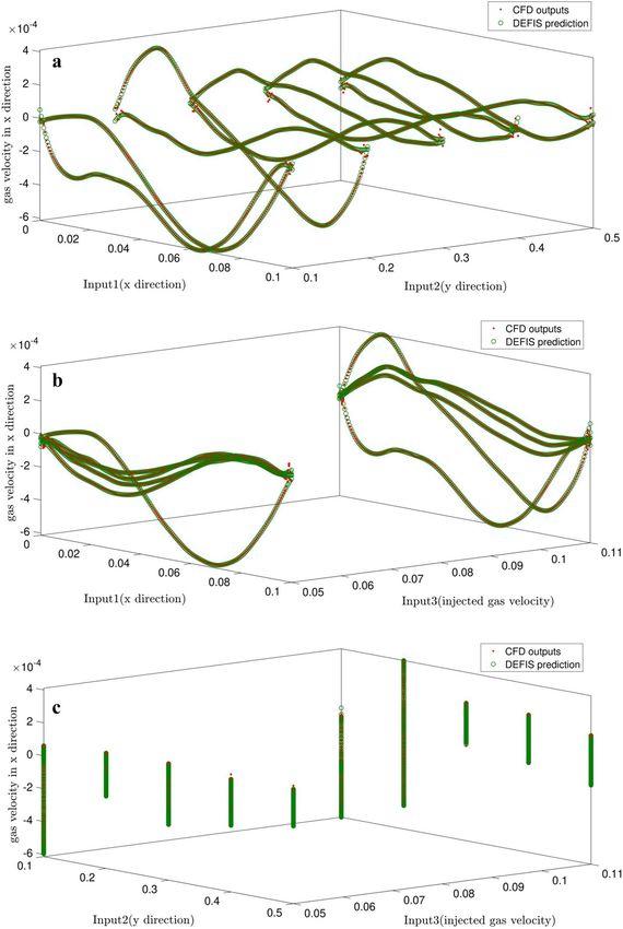
www.nature.com/scientificreports/
Methodology
CFD approach. Here, Euler–Euler (E–E) multiphase method is employed to evaluate the average mass,
energy, and flow equations separately for each phase along with the volume fraction equation. Indeed, E–E
procedure treats individual phase as interpenetrating continua, thereby volume fractions are taken as space and
time function and their sum equals to 1. The equation of E–E is given as f ollows34,35:
Continuity equation35:
∂
(ρk εk ) + ∇(ρk εk uk ) = 0. (1)
∂t
To compute the momentum equation, all interfacial forces (e.g. drag, turbulent dispersion, lift, vertical mass,
and wall lubrications) are combined. Equation (2) describes the momentum transfer35:
∂
(ρk εk uk ) + ∇.(ρk εk uk uk ) = − ∇.(εk τk ) − εk ∇ρ + εk ρk g + MI,K . (2)
∂t
The following equation interprets the stress term of bubbles and liquid phase as 35:
2
τk = −µeff,k (∇uk ) + (∇uk )T − I(∇.uk ). (3)
3
where µeff,k stands the effective viscosity. Detailed description of the models’ equations are reported
elsewhere8,16,36–39.
Takagi, Sugeno, and Kang, fuzzy inference system (FIS). In prior works, the fuzzy controller and
types of fuzzy inference system have been fully explained to optimize the processes in nature or presented as a
problem solver. For instance, Takagi, Sugeno, and Kang have designed the structure of FIS, which translate the
conceptual understanding of human in making decisions40–42. This type of structure can be coupled to other
learning formats for better decision in the physical processes that human needs computational calculation for
several problems. Different learning framework can learn the dataset with different algorithms and data rand-
omization selection within the frame of fuzzy. These learning processes can also have a different level of model
accuracy or training time. In the current study, we used different algorithms to investigate the ability of each of
them separately. Also, the ability of training, as well as the ability of the decision in the fuzzy logic system were
combined to prediction the model. We employed DE method to train the system, and after that, the data were
used fuzzy logic for the prediction. For better comparing the accuracy of the model, we used ANFIS, or ACO to
complete the training. After the methods were combined with the fuzzy logic system, we can have our model for
the purpose of prediction. We completed the training from all of the obtained models in the form of iterative in
AI, and the iterative part of the model is called an iteration. After solving for the iterative according to the con-
vergence and error criteria, we stop the system for solving the iterative. The data in training and the intelligence
in the training process were combined with the fuzzy logic system to provide the predictions.
The antecedents and membership functions are very identical with the Mamdani FIS structure, while the
polynomial consequent can be used and replaced with fuzzy framework. In addition, a Mamdani FIS structure
can be observed as a 0-th order TSK FIS. The TSK rule framework can be described, such as following43:
Ri : IF x1 is Ai1 and . . . and xn is Ain THEN y = Ci1 ∗ x1 + · · · Cin ∗ xn + Cin + 1 (4)
One of the main abilities over the Mamdani model is about small number of rules in the main structure of
the model. On the other hand, we can distinguish between various FIS structures based on the weighted average
of the rule output parameters rather than the max operator m echanism44. This model behavior and connection
in the FIS structure can be observed in the framework of TSK. Additionally, the rule output can provide less
computational cost and efforts due to defuzzification calculation in the model of AI. This model is also known
as Sugeno m odel43.
One of the commonly used popular computing frameworks is the Takagi, Sugeno, and Kang (TSK) fuzzy
inference system (FIS), which is based on theory of fuzzy set, fuzzy reasoning, and if–then rule. This framework
has been effectively used in areas like data classification and expert systems. In terms of fuzzy reasoning, Takagi
and Sugeno introduced if–then rules for construction of FIS architecture45. Here, x direction, y direction and
injected gas velocity are assumed as FIS inputs to achieve gas phase velocity in x coordinate as FIS output.
For each input parameter fuzzy process generates the behavior of membership function as a function of input
parameters that defines the connectivity between input parameters and the complexity of parameters within
the domain of fuzzy rules. Input selection and associated dataset for each input during learning can be fully
coupled with number of membership functions or types of function that describes the degree of membership
functions in each input. w i can also be calculated in the model and show the rule strength of the ith rule R i. wi
can be described for different input parameters, such as X, Y and Vg and written as46:
wi = µAi (X)µBi (Y)µCi (Vg ) (5)
where μAi, μBi and μCi explain signals from implemented membership functions (MFs) on inputs, x coordina-
tion (X), y coordination (Y) and injected gas velocity ( Vg). In Eq. (5), each input parameter, such as location of
computing nodes and gas velocity, can be defined in the training mode.
The relative firing strength in each rule is achieved and the fuzzy-model output f i is computed by a weighted
mean(WM) defuzzification as f ollows15:
Scientific Reports | (2021) 11:2380 | https://doi.org/10.1038/s41598-021-81957-3 3
Vol.:(0123456789)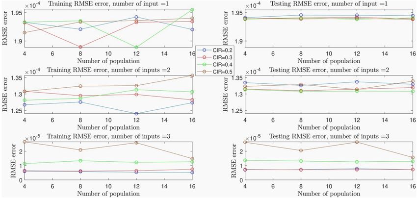
www.nature.com/scientificreports/
Method DEFIS ACOFIS ANFIS
Number of inputs 3 3 3
Number of P (%) 65 65 65
FIS parameters
Clustering Type Subtractive clustering Subtractive clustering Subtractive clustering
FIS type Sugeno Sugeno Sugeno
Cluster influence
0.2 0.2 0.2
range (CIR)
Type of input mem-
guassmf guassmf guassmf
bership function
Subtractive clustering Type of output mem-
parameters Linear Linear Linear
bership function
Squash factor 1.25 1.25 1.25
Accept ratio 0.5 0.5 0.5
Reject ratio 0.15 0.15 0.15
Number of population 16 Number of ants 10 – –
Algorithms important parameters Crossover probability 0.5 Pheromone effect 0.5 – –
Number of rule 64 Number of rule 64 Number of rule 65
Maximun of training
150 150 150
iteration
Error goal 0 0 0
Training options
Initial step size 0.01 0.01 0.01
Step size decrease 0.9 0.9 0.9
Step size increase 1.1 1.1 1.1
Table 1. DEFIS, ACOFIS, ANFIS set parameters for learning processes.
wi fi = wi (pi X + qi Y + ri Vg + si ) (6)
where pi, qi, ri, and s i are defined as the if–then rules’ parameters known as consequent parameters. The signals
are aggregated to yield the output of model, and represent the estimation result. With the aim of updating the
parameters, a hybrid learning algorithm is employed where gradient descent technique updates the MFs param-
eters and Least Square Estimate (LSE) tecnique updates consequent factors.
Differential evolution (DE) algorithm. Price and S torn47 developed differential evolution (DE) algo-
rithm as a breakthrough algorithm. It is developed for global optimization problems of continuous domains with
3 control search parameters, i.e.:
1. F: mutation control parameter, which is for control of the extent to which the differential variation is ampli-
fied.
2. CR: the crossover control parameter as a constant parameters to determine what parameter associates with
what trial vector parameter in the crossover operation.
3. NP: the size of population, which is the number of individuals in the population.
Several studies were conducted on DE and its applications46–51 and recommended value ranges for F, CR, and
NP50. These factors indicate if the algorithm is able to find a near-optimum solution effectively or not. Adopting
the right value using trial–error approach takes a large amount of t ime52,53. There are several studies on the effect
of these parameters on the performance of DE52.
By adding tolerances as two novel parameters and taking the diversity of the population into account, we can
adjust the amounts of the mutation control parameter and the crossover control parameters to achieve a higher
algorithm efficiency and improve the quality of solution49. In54, a self-adaptive method was proposed to estimate
DE parameters, the crossover parameters, and the mutation amplification. The way these 3 control parameters
affect the DE performance was illustrated b y48 by performing experiment on test functions. Consequently, new
solutions to improve the effectiveness, robustness, and efficiency were found by adopting better approaches to
set the DE’s search control parameter values.
Geometrical structure. In this work, a cylindrical-based bubble column with height and diameter of
162 cm and 10 cm, respectively was simulated. The column also features two nozzles of 0.9 cm diameter and
5 cm higher than the bottom plate of the column. The liquid–gas dispersion was heated by an electrical heater
and the superficial gas velocity was equal to 0.05 m/s.
Boundary conditions and numerical methods. The simulations were done in ANSYS-Fluent on the
basis of superficial gas velocity, the gas velocity from each sparger orifice was calculated. The bubble column out-
let is featured with degassing boundary condition. Non-slip and free slip boundary conditions are implemented
Scientific Reports | (2021) 11:2380 | https://doi.org/10.1038/s41598-021-81957-3 4
Vol:.(1234567890)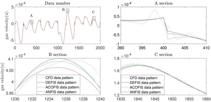
www.nature.com/scientificreports/
Figure 1. DEFIS learning processes with changes in the number of population as DE algorithm parameter and
cluster influence range (CIR) as subtractive clustering parameter.
Figure 2. DE training and testing processes when CIR is 0.2, and number of input is 3.
at the wall edge, on the liquid and gas bubbles, respectively. These conditions are offered by former studies54–57.
In practice, the bubbles are under no fraction from the wall and it can travel along the boundary wall with no
limitation. Therefore, it is assumed that there are almost not contact between the b ubbles58.
Here, the control volume method was used to discretize the conservation equations. Generally, the flow
field can be obtained using a variety of solution procedures like finite difference59,60, Lattice Boltzmann60–64, and
finite volume method38,64–67. The most reliable and robust technique, which was used by CFX is finite volume
discretization. This approach is capable of yielding the single/multiphase flow, and heat/mass transfer within
an arbitrary geometry with or without structured g rid38,64–69. The technique has been used by several studies to
obtain the flow regime and gas dynamics through the reactor38,39,65,66,70. It is possible to solve the equation system
using the SIMPLEC procedure. Because of the decrement in numerical diffusion and dispersion in the Eulerian
framework, it is possible to employ the Total Variation Diminishing (TVD) in the numerical m ethod65,66,70–73.
Bubbling flow computation is done for 1400 s, and all CFD studies used time step of 0.1, which was deter-
mined based on the reality that the maximum courant-Friedrichs-Levy (CFL) number should be smaller than 1.
Some reports are existed that with CFL < 1, the numerical method gives accurate predictions of the multiphase
features and better refinement of time step does not result in notable changes of the flow pattern result. In addi-
tion, CFL > 1 leads to inaccurate p redictions13,74–80.
Scientific Reports | (2021) 11:2380 | https://doi.org/10.1038/s41598-021-81957-3 5
Vol.:(0123456789)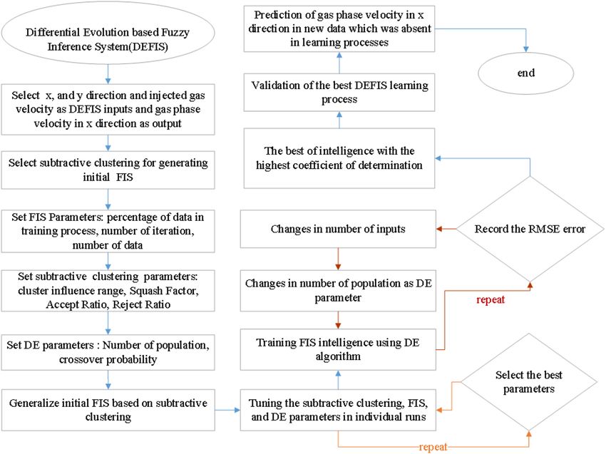
www.nature.com/scientificreports/

                                            Figure 3.  FIS system schematics when number of input is 3, and number of rule for each input membership
                                            function is 64.

                                            Results and discussion
                                            Here, DE algorithm is applied in the FIS training step in order to reach the best FIS Capacity. The number of
                                            extracted data is 2000 that was obtained when the injected gas velocity from bottom of the reactor was 0.05 and
                                            0.11 (m/s). Each data consists of characteristics of fluids including x and y direction, injected gas velocity (FIS
                                            inputs), and gas phase velocity in x direction (FIS output). The amount of data applied in the training step is
                                            65% and the maximum FIS iteration is 150 and also the type of clustering is subtractive clustering. Changes in
                                            some parameters like the number of inputs and cluster influence range (CIR), which is a parameter of FIS and
                                            the number of population, which is a parameter of DE algorithm were examined. To begin we did the learning
                                            processes with one input and CIR = 0.5, 0.4, 0.3 and 0.2 by considering number of population = 4, 8, 12, and 16
                                            for each CIR, respectively. Results in Table S1, Appendix, show that when the number of input is 1 changes in
                                            amount of CIR and number of population had not any considerable changes in the amount of RMSE error for
                                            training and testing steps, and the lowest amount of RMSE for training is 0.00192 and for testing is 0.000194 in
                                            another word, percentage of FIS Capacity is about 29%.
                                                To reach an enormous capacity of prediction, the second FIS input was considered. By repeating training
                                            as well as testing steps for a diversity of CIR and number of population, the amount of RMSE error declined to
                                            0.000127 for training process and 0.000132 for testing process which indicates that we achieved 77% of intel-
                                            ligence. This significant positive change in FIS Capacity suggests that increasing the number of inputs has the
                                            maximum positive effect on FIS Capacity in comparison with other variable parameters (see Table S2, Appendix).
                                                The best FIS Capacity was achieved that is 99.9% by adding injected gas velocity as third input and repetition
                                            of training and testing steps for a different range of CIR and the number of population. Table S3 (Appendix)
                                            indicates the amount of RMSE for training process declined to 5.2E−06 and for testing process declined to
                                            7.2E−06. This amount was obtained when CIR = 2 and number of population was 16.
                                                All initial and tuning parameters for DEFIS, ACOFIS, and ANFIS method are described in Table 1. This table
                                            shows that the number of input parameters for all methods is identical (number of inputs = 3), and the percent-
                                            age of training data is 65% of whole datasets. In the FIS section, the clustering type and FIS type is Subtractive
                                            Clustering and Sugeno, respectively. In the Subtractive Clustering section, more effective tuning parameters can
                                            be selected. In this part, CIR, type of input membership function, type of output membership function, Squash
                                            factor, Accept and Reject ratio are 0.2, guassmf, linear, 1.25, 0.5, and 0.15, respectively. Tuning parameters that
                                            have a big impact on the model are selected in the next stage, which are specific model parameters for each pre-
                                            diction model. For the DEFIS model, the number of population, Crossover Probability, and the number of the
                                            rule are 16, 0.5, 64, respectively. However, in the ACOFIS method, different parameters are used in the model,
                                            such as the number of ants = 10, pheromone effect = 0.5, and the number of rules equal to 64. In the final stage
                                            in the ANFIS method, only a number of rules can be designed in the model, and it is 65. For the final stage of
                                            modeling parameters, all parameters are similar. In this regard, the maximum of training iteration, Error Goal,
                                            Initial Step Size, Step Size Decrease and Step Size Increase is 150, 0, 0.01, 0.9, and 1.1, respectively.
                                                Figure 1 illustrates the effects of population, the number of CIR, and the number of input on the RMSE error
                                            of the system. We also consider the error in the testing/training steps. As shown, when the number of input is one,
                                            that is a very low number; a meaningful effect is not seen for the number of CIR and the number of population in
                                            both testing and training processes. Nevertheless, by increasing the number of inputs, the system reaches a sig-
                                            nificant intelligence, and the effect of the number of CIR becomes meaningful. Moreover, the effect of the number
                                            of population on RMSE error improves in both testing and training. For instance, Fig. 1 for number of inputs = 3
                                            shows when the number of CIR is low, including 0.2, and 0.3, the error is in its lowest amount. This shows that
                                            the system has a very low amount of error, as well as a low CIR number. After studying the RMSE error, we fixed
                                            the system with the lowest RMSE error, which is the best system regarding the statistics and error. After that, we
                                            study the system in regression and pattern recognition domains to see how the system can predict our model.

          Scientific Reports |   (2021) 11:2380 |                https://doi.org/10.1038/s41598-021-81957-3                                                  6

Vol:.(1234567890)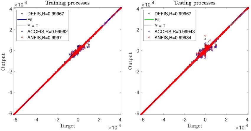
www.nature.com/scientificreports/
Figure 4. (a) Comparison of gas velocity between CFD output and DEFIS prediction with considering first and
second inputs. (b) Comparison of gas velocity between CFD output and DEFIS prediction with considering first
and third inputs. (c) Comparison of gas velocity between CFD output and DEFIS prediction with considering
second and third inputs.
Figure 2 shows that the value of regression ( R2) for both training and testing processes is more 99.9%. Accord-
ing to the FIS structure number of rules is 64 for each input, hidden layer of FIS and output equally which is
depicted in Fig. 3.
For intelligence validation, data involved in the learning step are predicted and compared with the CFD
results, there is a good adaptation between them and it is depicted in Fig. 4a–c. Moreover, by employing FIS struc-
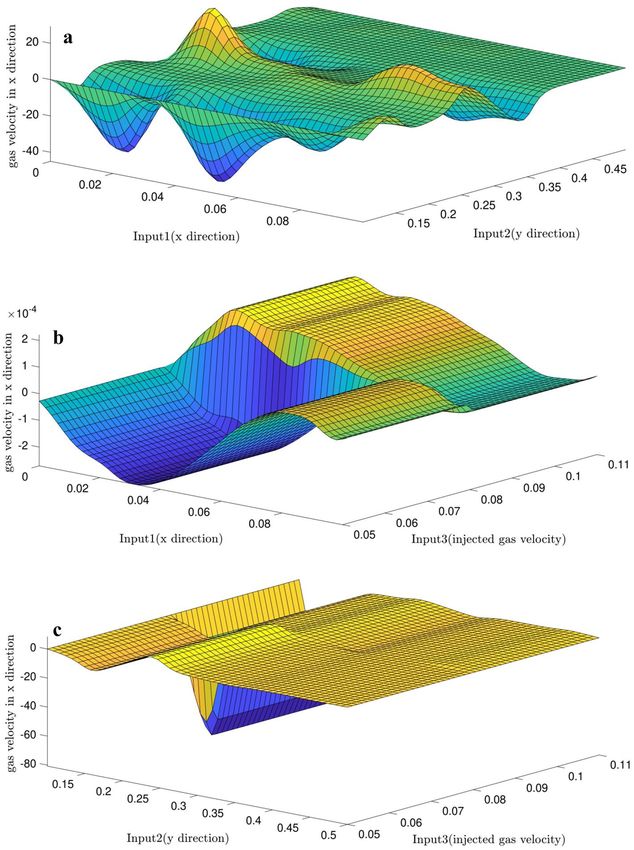
ture, surfaces are predicted based on the inputs which are depicted in Fig. 5a–c. By implementing 2 of the inputs,
gas phase velocity in x direction as the FIS output can be extracted via predicted surfaces obtained in Fig. 5.
The implemented data in the learning processes were extracted when the velocity of injected gas from bottom
of the reactor was 0.05 and 0.11 (m/s). Furthermore, in this work by implementing FIS structure that is combined
with DE algorithm in training process, extracted data from situation that the velocity of injected gas from bottom
Scientific Reports | (2021) 11:2380 | https://doi.org/10.1038/s41598-021-81957-3 7
Vol.:(0123456789)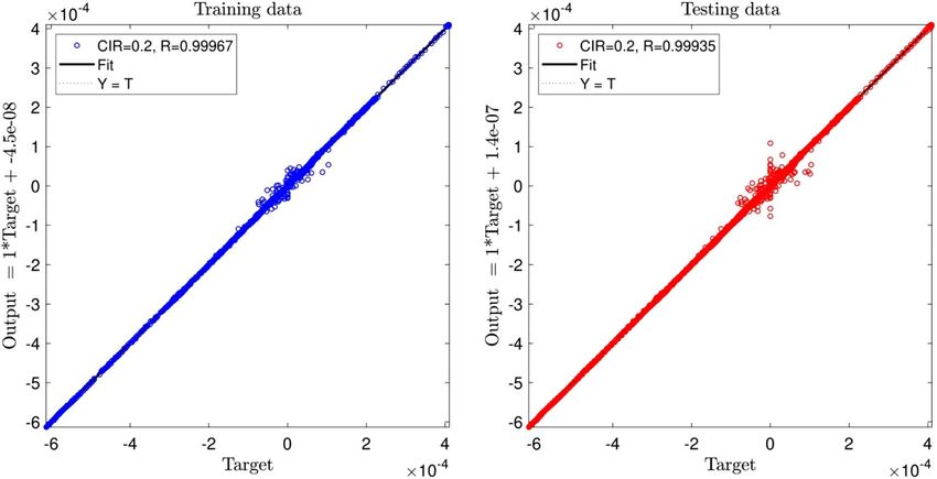
www.nature.com/scientificreports/
Figure 5. (a) Gas velocity predicted surface with considering first and second inputs. (b) Gas velocity predicted
surface with considering first and third inputs. (c) Gas velocity predicted surface with considering second and
third inputs.
of reactor was 0.08 (m/s) was predicted. Predicted new data was compared with the previous predicted data,
which is depicted in Fig. 6a–c, the left side of Fig. 6 show comparison of predicted data with the included CFD
data in the learning processes while the right side of Fig. 6 show comparison of predicted new data with the CFD
new data that were absent in the learning processes. As can be clearly seen from Fig. 7, there is an adaptation
between vectors of predicted gas phase velocity in x direction as the output of artificial intelligence and vectors
of absent CFD data in the learning processes.
Figure 8 shows the best system in terms of the error. We study the system with the CIR number of 0.2 and
the number of population at its highest level. Also, we study the DE model with other methods, including the
ANFIS and ant optimization methods, to see how the error of the system could be similar to other conventional
AI models. The figure shows the regression of the system and indicates the DE model has a good prediction,
which is very similar to the ACO method. The methods can predict the dataset, and the highest amount of R 2
is achieved, which is 0.99.
After studying the regression of the system, we consider the pattern recognition because the accuracy and
exactness of the regression of RMSE error and average error are not exact criteria for the prediction of a model.
We need to study the flow and CFD patterns point by point to see how the model could be predicted. To do so,
we used ANFIS and ACO methods to compare their ability with the DE model. As shown in Fig. 9, the DE model
Scientific Reports | (2021) 11:2380 | https://doi.org/10.1038/s41598-021-81957-3 8
Vol:.(1234567890)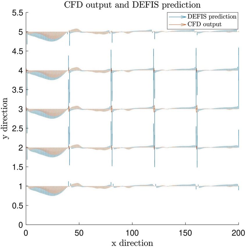
www.nature.com/scientificreports/

                                  Figure 6.  (a) Comparison of predicted gas velocity and CFD output (gas velocity) which is present in DEFIS
                                  learning (in left figure) and comparison of predicted gas velocity and CFD output (gas velocity) which is absent
                                  in DEFIS learning (the right figure) (with considering inputs 1 and 2). (b) Comparison of predicted gas velocity
                                  and CFD output (gas velocity) which is present in DEFIS learning (in left figure) and comparison of predicted
                                  gas velocity and CFD output (gas velocity) which is absent in DEFIS learning (in right figure) (with considering
                                  inputs 1 and 3). (c) Comparison of predicted gas velocity and CFD output (gas velocity) which is present in
                                  DEFIS learning (in left figure) and comparison of predicted gas velocity and CFD output (gas velocity) which is
                                  absent in DEFIS learning (in right figure) (with considering inputs 2 and 3).

Scientific Reports |   (2021) 11:2380 |               https://doi.org/10.1038/s41598-021-81957-3                                                 9

                                                                                                                                            Vol.:(0123456789)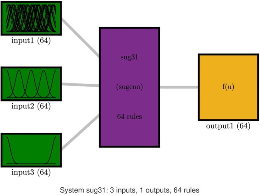
www.nature.com/scientificreports/

                                            Figure 7.  Comparison of gas velocity between predicted output via DEFIS and CFD output, x direction is
                                            number of data (node) and y direction is different heights.

                                            Figure 8.  Correlation coefficient of DEFIS, ACOFIS, and ANFIS methods for training and testing processes
                                            after achieving the best intelligence.

                                            could suitably predict the gas velocity pattern for all of the numbers of data, and the flow pattern matches with
                                            CFD dataset. Moreover, the pattern is also very similar to CFD and ACO. In general, the method of DE contains
                                            a good ability of flow characteristics prediction and gas–liquid flow patterns. This method is also very similar to
                                            ANFIS and ACO with regards to pattern prediction in the domain.
                                                To fully illustrate the main flow chart of the current methodology (algorithm) and show how model param-
                                            eters can impact on the final level of model accuracy and prediction capability, the main flow chart of this research
                                            is shown in Fig. 10. Figure 10 shows that x and y computing nodes and inlet gas velocity (gas sparge into the
                                            reactor) are used as input training, and gas velocity distribution as an output dataset. In the second level of the
                                            model, the FIS structure is selected based on subtractive clustering for the decision part of the model. As an
                                            initial point of running model number of iteration (epoch number), the percentage of gathering datasets and the
                                            total number of data are selected in the algorithm. Then to generate the subtractive clustering framework, several
                                            parameters are selected, such as cluster influence range, squash factor, aspect ratio, and reject ratio. After the
                                            development of subtractive clustering mode, DE parameters (number of population and crossover probability)
                                            can be defined in the model structure. We can also generalize the initial FIS structure. Then the tuning part is

          Scientific Reports |   (2021) 11:2380 |                https://doi.org/10.1038/s41598-021-81957-3                                                   10

Vol:.(1234567890)
www.nature.com/scientificreports/
Figure 9. Pattern recognition for different methods such as ANFIS, DEFIS and ACOFIS.
Figure 10. Flowchart of DEFIS method.
activated for FIS, subtractive clustering, and DE parameters. In this stage of the model, the code is evaluated
for the high level of accuracy and prediction capability. Then the training campaign is started, while the RSME
error is fully conducted to evaluate the high level of accuracy. In each step, if the RSME value cannot present
the accurate model, the model is changed with other model parameters. In this part of the code, the number
of population and number of input parameters can be changed to get the best level of accuracy and prediction
capability. Then the final stage of code is activated to assess the level of accuracy, validate the model, and compare
the model in predicting “non-training” datasets.
Scientific Reports | (2021) 11:2380 | https://doi.org/10.1038/s41598-021-81957-3 11
Vol.:(0123456789)www.nature.com/scientificreports/
Conclusions
In this study, prediction of gas phase velocity in the reactor via a combination of DE algorithm and Capacity of
FIS was studied and changes in DE algorithm and FIS parameters were examined. Learning data was extracted
when injected gas velocity in bottom of the reactor was 0.05 and 0.11 (m/s). By Capacity of FIS , we could com-
pletely predict gas phase velocity in x direction when injected gas velocity was between 0.05 and 0.11 (m/s) even-
tually 0.08 was selected and prediction process was done which shows capability of the artificial intelligence in
predicting gas-phase velocity in different amount of injected gas velocity in bottom of the reactor. By comparing
different types of clustering data including grid partition, subtractive and fuzzy c-mean for achieving the highest
percentage of intelligence is appreciable in the future study. Comparing several algorithms (such as ANFIS Ant
Colony and DE), we can conclude that the DE algorithms have high potentiality in predicting the CFD data. This
algorithm can suitably complete the training process; moreover, it can complete the prediction process when
the fuzzy logic system also exists in the system. Also, this algorithm can be used in pattern recognition that can
match the prediction data in the target data or CFD data. We can see that CFD and DE patterns match each other.
For future studies, using other algorithms in the training that have high potentiality seems to be advantageous.
They can also have high potentiality in speeding up the learning process; therefore, we must examine them to
find the best and fastest algorithm in the learning process. These algorithms can be used in different physical
conditions, and their potentiality could be examined in a wide range of applications.
Received: 26 May 2020; Accepted: 5 January 2021
References
1. Chaumat, H., Billet, A.-M. & Delmas, H. Hydrodynamics and mass transfer in bubble column: Influence of liquid phase surface
tension. Chem. Eng. Sci. 62, 7378–7390 (2007).
2. Ranade, V. V. Computational Flow Modeling for Chemical Reactor Engineering Vol. 5 (Elsevier, Amsterdam, 2001).
3. Tisnadjaja, D., Gutierrez, N. A. & Maddox, I. S. Citric acid production in a bubble-column reactor using cells of the yeast Can-
didaguilliermondii immobilized by adsorption onto sawdust. Enzyme Microb. Technol. 19, 343–347 (1996).
4. Babanezhad, M., Nakhjiri, A. T., Rezakazemi, M. & Shirazian, S. Developing intelligent algorithm as a machine learning overview
over the big data generated by Euler–Euler method to simulate bubble column reactor hydrodynamics. ACS Omega 5, 20558–20566
(2020).
5. Deckwer, W.-D. & Field, R. W. Bubble Column Reactors Vol. 200 (Wiley, New York, 1992).
6. Xiao, Q., Wang, J., Yang, N. & Li, J. Simulation of the multiphase flow in bubble columns with stability-constrained multi-fluid
CFD models. Chem. Eng. J. 329, 88–99 (2017).
7. Jakobsen, H. A., Lindborg, H. & Dorao, C. A. Modeling of bubble column reactors: Progress and limitations. Ind. Eng. Chem. Res.
44, 5107–5151 (2005).
8. Zhang, D. Eulerian modeling of reactive gas-liquid flow in a bubble column, 128 (2007).
9. Vaidheeswaran, A. & de Bertodano, M. L. Stability and convergence of computational eulerian two-fluid model for a bubble plume.
Chem. Eng. Sci. 160, 210–226 (2017).
10. McClure, D. D., Kavanagh, J. M., Fletcher, D. F. & Barton, G. W. Development of a CFD model of bubble column bioreactors: Part
one—a detailed experimental study. Chem. Eng. Technol. 36, 2065–2070 (2013).
11. Hlawitschka, M., Kováts, P., Zähringer, K. & Bart, H.-J. Simulation and experimental validation of reactive bubble column reactors.
Chem. Eng. Sci. 170, 306–319 (2017).
12. Tian, E., Babanezhad, M., Rezakazemi, M. & Shirazian, S. Simulation of a bubble-column reactor by three-dimensional CFD:
Multidimension-and function-adaptive network-based fuzzy inference system. Int. J. Fuzzy Syst. 22, 1–14 (2019).
13. Xu, P., Babanezhad, M., Yarmand, H. & Marjani, A. Flow visualization and analysis of thermal distribution for the nanofluid by
the integration of fuzzy c-means clustering ANFIS structure and CFD methods. J. Vis. 23, 97–110 (2020).
14. Shamshirband, S. et al. Prediction of flow characteristics in the bubble column reactor by the artificial pheromone-based com-
munication of biological ants. Eng. Appl. Comput. Fluid Mech. 14, 367–378 (2020).
15. Babanezhad, M., Rezakazemi, M., Hajilary, N. & Shirazian, S. Liquid-phase chemical reactors: Development of 3D hybrid model
based on CFD-adaptive network-based fuzzy inference system. Can. J. Chem. Eng. 97, 1676–1684 (2019).
16. Babanezhad, M., Nakhjiri, A. T. & Shirazian, S. Changes in the number of membership functions for predicting the gas volume
fraction in two-phase flow using grid partition clustering of the ANFIS method. ACS Omega 5, 16284–16291 (2020).
17. Cao, Y., Babanezhad, M., Rezakazemi, M. & Shirazian, S. Prediction of fluid pattern in a shear flow on intelligent neural nodes
using ANFIS and LBM. Neural Comput. Appl. 32, 13313–13321 (2020).
18. Nabipour, N., Babanezhad, M., Taghvaie Nakhjiri, A. & Shirazian, S. Prediction of nanofluid temperature inside the cavity by
integration of grid partition clustering categorization of a learning structure with the fuzzy system. ACS Omega 5, 3571–3578
(2020).
19. Barchi, A. C. et al. Artificial intelligence approach based on near-infrared spectral data for monitoring of solid-state fermentation.
Process Biochem. 51, 1338–1347 (2016).
20. Halim, Z., Kalsoom, R., Bashir, S. & Abbas, G. Artificial intelligence techniques for driving safety and vehicle crash prediction.
Artif. Intell. Rev. 46, 351–387 (2016).
21. Suman, S., Khan, S., Das, S. & Chand, S. Slope stability analysis using artificial intelligence techniques. Nat. Hazards 84, 727–748
(2016).
22. Zahraee, S., Assadi, M. K. & Saidur, R. Application of artificial intelligence methods for hybrid energy system optimization. Renew.
Sustain. Energy Rev. 66, 617–630 (2016).
23. Zadeh, L. A. Fuzzy sets. Inf. Control 8, 338–353 (1965).
24. Adnan, M. M., Sarkheyli, A., Zain, A. M. & Haron, H. Fuzzy logic for modeling machining process: A review. Artif. Intell. Rev. 43,
345–379 (2015).
25. Azadegan, A., Porobic, L., Ghazinoory, S., Samouei, P. & Kheirkhah, A. S. Fuzzy logic in manufacturing: A review of literature and
a specialized application. Int. J. Prod. Econ. 132, 258–270 (2011).
26. Koukol, M., Zajíčková, L., Marek, L. & Tuček, P. Fuzzy logic in traffic engineering: A review on signal control. Math. Probl. Eng.
2015, 1–14 (2015).
27. Lochan, K. & Roy, B. Proceedings of Fourth International Conference on Soft Computing for Problem Solving 499–511 (Springer,
New York, 2015).
Scientific Reports | (2021) 11:2380 | https://doi.org/10.1038/s41598-021-81957-3 12
Vol:.(1234567890)www.nature.com/scientificreports/
28. Suganthi, L., Iniyan, S. & Samuel, A. A. Applications of fuzzy logic in renewable energy systems—A review. Renew. Sustain. Energy
Rev. 48, 585–607 (2015).
29. Marani, M., Songmene, V., Zeinali, M., Kouam, J. & Zedan, Y. Neuro-fuzzy predictive model for surface roughness and cutting
force of machined Al-20 Mg 2 Si–2Cu metal matrix composite using additives. Neural Comput. Appl. 32, 8115–8126 (2020).
30. Pourtousi, M., Zeinali, M., Ganesan, P. & Sahu, J. Prediction of multiphase flow pattern inside a 3D bubble column reactor using
a combination of CFD and ANFIS. RSC Adv. 5, 85652–85672 (2015).
31. Castillo, O. et al. Comparative study in fuzzy controller optimization using bee colony, differential evolution, and harmony search
algorithms. Algorithms 12, 9 (2019).
32. Castillo, O. et al. Shadowed type-2 fuzzy systems for dynamic parameter adaptation in harmony search and differential evolution
algorithms. Algorithms 12, 17 (2019).
33. Castillo, O. et al. A high-speed interval type 2 fuzzy system approach for dynamic parameter adaptation in metaheuristics. Eng.
Appl. Artif. Intell. 85, 666–680 (2019).
34. Mousazadeh, F., van den Akker, H. & Mudde, R. Eulerian simulation of heat transfer in a trickle bed reactor with constant wall
temperature. Chem. Eng. J. 207, 675–682 (2012).
35. Pourtousi, M., Ganesan, P. & Sahu, J. Effect of bubble diameter size on prediction of flow pattern in Euler–Euler simulation of
homogeneous bubble column regime. Measurement 76, 255–270 (2015).
36. Pourtousi, M., Sahu, J. & Ganesan, P. Effect of interfacial forces and turbulence models on predicting flow pattern inside the bubble
column. Chem. Eng. Process. 75, 38–47 (2014).
37. Li, G., Yang, X. & Dai, G. CFD simulation of effects of the configuration of gas distributors on gas–liquid flow and mixing in a
bubble column. Chem. Eng. Sci. 64, 5104–5116 (2009).
38. Tabib, M. V., Roy, S. A. & Joshi, J. B. CFD simulation of bubble column—An analysis of interphase forces and turbulence models.
Chem. Eng. J. 139, 589–614 (2008).
39. Silva, M. K., d’Ávila, M. A. & Mori, M. Study of the interfacial forces and turbulence models in a bubble column. Comput. Chem.
Eng. 44, 34–44 (2012).
40. Precup, R.-E., David, R.-C., Petriu, E. M., Preitl, S. & Radac, M.-B. Fuzzy control systems with reduced parametric sensitivity based
on simulated annealing. IEEE Trans. Ind. Electron. 59, 3049–3061 (2011).
41. Peraza, C., Valdez, F. & Melin, P. Optimization of intelligent controllers using a type-1 and interval type-2 fuzzy harmony search
algorithm. Algorithms 10, 82 (2017).
42. Fierro, R. & Castillo, O. Recent Advances on Hybrid Intelligent Systems 81–88 (Springer, New York, 2013).
43. Yen, J. & Langari, R. Fuzzy Logic: Intelligence, Control, and Information Vol. 1 (Prentice Hall, Upper Saddle River, 1999).
44. Babanezhad, M. et al. Liquid temperature prediction in bubbly flow using ant colony optimization algorithm in the fuzzy inference
system as a trainer. Sci. Rep. 10(1), (2020).
45. Takagi, T. & Sugeno, M. Fuzzy identification of systems and its applications to modeling and control. IEEE Trans. Syst. Man Cybern.,
116–132 (1985).
46. Rezakazemi, M. & Shirazian, S. Gas-liquid phase recirculation in bubble column reactors: Development of a hybrid model based
on local CFD—Adaptive Neuro-Fuzzy Inference System (ANFIS). J. Non-Equilib. Thermodyn. 44, 29–42. https://doi.org/10.1515/
jnet-2018-0028 (2019).
47. Storn, R. & Price, K. Differential evolution—a simple and efficient adaptive scheme for global optimization over continuous spaces.
Technical Report, International Computer Science Institute, 1–12 (1995).
48. Liu, J. in Proceedings of the 8th International Conference on Soft Computing (MENDEL 2002), 11–18.
49. Cruz, I. L., Van Willigenburg, L. & Van Straten, G. in Proceedings of the IASTED International Conference" Artificial Intelligence
and Soft Computing", Cancun, Mexico, May 21–24, 2001. 211–216.
50. Storn, R. in Proceedings of North American Fuzzy Information Processing, 519–523 (IEEE).
51. Storn, R. & Price, K. Differential evolution—A simple and efficient heuristic for global optimization over continuous spaces. J.
Glob. Optim. 11, 341–359 (1997).
52. Ochoa, P., Castillo, O. & Soria, J. Optimization of fuzzy controller design using a Differential Evolution algorithm with dynamic
parameter adaptation based on Type-1 and Interval Type-2 fuzzy systems. Soft. Comput. 24, 193–214 (2020).
53. Lampinen, J. & Zelinka, I. in Proceedings of MENDEL, 76–83.
54. Abbass, H. A. in Proceedings of the 2002 Congress on Evolutionary Computation, 831–836.
55. Monahan, S. M., Vitankar, V. S. & Fox, R. O. CFD predictions for flow-regime transitions in bubble columns. AIChE J. 51,
1897–1923 (2005).
56. Frank, T., Zwart, P., Krepper, E., Prasser, H.-M. & Lucas, D. Validation of CFD models for mono-and polydisperse air–water two-
phase flows in pipes. Nucl. Eng. Des. 238, 647–659 (2008).
57. Díaz, M. E. et al. Numerical simulation of the gas–liquid flow in a laboratory scale bubble column: Influence of bubble size distri-
bution and non-drag forces. Chem. Eng. J. 139, 363–379 (2008).
58. Rzehak, R. & Krepper, E. CFD modeling of bubble-induced turbulence. Int. J. Multiph. Flow 55, 138–155 (2013).
59. Alhumaizi, K. Comparison of finite difference methods for the numerical simulation of reacting flow. Comput. Chem. Eng. 28,
1759–1769 (2004).
60. Nakhjiri, A. T. & Roudsari, M. H. Modeling and simulation of natural convection heat transfer process in porous and non-porous
media. Appl. Res. J. 2, 199–204 (2016).
61. Sheldareh, A., Safdari, A., Pourtousi, M. & Sidik, N. Prediction of particle dynamics in lid-driven cavity flow. Int. Rev. Model. Simul.
5, 1344–1347 (2012).
62. Azwadi, C., Razzaghian, M., Pourtousi, M. & Safdari, A. Numerical prediction of free convection in an open ended enclosure using
lattice Boltzmann numerical method. Int. J. Mech. Mater. Eng 8, 58–62 (2013).
63. Pourtousi, M., Razzaghian, M., Safdari, A. & Darus, A. N. Simulation of fluid flow inside a back-ward-facing step by MRT-LBM.
Int. Proc. Comput. Sci. Inf. Technol 33, 130–135 (2012).
64. Razzaghian, M., Pourtousi, M. & Darus, A. N. in Thailand: International Conference on Mechanical and Robotics Engineering.
65. Pfleger, D. & Becker, S. Modelling and simulation of the dynamic flow behaviour in a bubble column. Chem. Eng. Sci. 56, 1737–1747
(2001).
66. Pfleger, D., Gomes, S., Gilbert, N. & Wagner, H.-G. Hydrodynamic simulations of laboratory scale bubble columns fundamental
studies of the Eulerian–Eulerian modelling approach. Chem. Eng. Sci. 54, 5091–5099 (1999).
67. Chen, P., Duduković, M. & Sanyal, J. Three-dimensional simulation of bubble column flows with bubble coalescence and breakup.
AIChE J. 51, 696–712 (2005).
68. Chen, P., Sanyal, J. & Duduković, M. Numerical simulation of bubble columns flows: Effect of different breakup and coalescence
closures. Chem. Eng. Sci. 60, 1085–1101 (2005).
69. Dhotre, M., Ekambara, K. & Joshi, J. CFD simulation of sparger design and height to diameter ratio on gas hold-up profiles in
bubble column reactors. Exp. Thermal Fluid Sci. 28, 407–421 (2004).
70. Pourtousi, M., Sahu, J., Ganesan, P., Shamshirband, S. & Redzwan, G. A combination of computational fluid dynamics (CFD) and
adaptive neuro-fuzzy system (ANFIS) for prediction of the bubble column hydrodynamics. Powder Technol. 274, 466–481 (2015).
71. Laborde-Boutet, C., Larachi, F., Dromard, N., Delsart, O. & Schweich, D. CFD simulation of bubble column flows: Investigations
on turbulence models in RANS approach. Chem. Eng. Sci. 64, 4399–4413 (2009).
Scientific Reports | (2021) 11:2380 | https://doi.org/10.1038/s41598-021-81957-3 13
Vol.:(0123456789)www.nature.com/scientificreports/
72. Deen, N. G., Solberg, T. & Hjertager, B. H. in Proceedings of 14th International Congress of Chemical and Process Engineering: CHISA
(Praha, Czech Republic, 2000).
73. Sokolichin, A. & Eigenberger, G. Gas–liquid flow in bubble columns and loop reactors: Part I. Detailed modelling and numerical
simulation. Chem. Eng. Sci. 49, 5735–5746 (1994).
74. Ma, T., Lucas, D., Ziegenhein, T., Fröhlich, J. & Deen, N. Scale-Adaptive Simulation of a square cross-sectional bubble column.
Chem. Eng. Sci. 131, 101–108 (2015).
75. Ziegenhein, T., Rzehak, R. & Lucas, D. Transient simulation for large scale flow in bubble columns. Chem. Eng. Sci. 122, 1–13
(2015).
76. Laín, S. Dynamic three-dimensional simulation of gas–liquid flow in a cylindrical bubble column. Latin Am. Appl. Res. 39, 317–326
(2009).
77. Buffo, A., Marchisio, D. L., Vanni, M. & Renze, P. Simulation of polydisperse multiphase systems using population balances and
example application to bubbly flows. Chem. Eng. Res. Des. 91, 1859–1875 (2013).
78. Dhotre, M., Deen, N., Niceno, B., Khan, Z. & Joshi, J. Large eddy simulation for dispersed bubbly flows: A review. Int. J. Chem.
Eng. 2013, 22 (2013).
79. Laín, S. Large eddy simulation of gas–liquid flow in a bubble column reactor. El Hombre y la Máquina 32, 108–118 (2009).
80. Dhotre, M. T., Niceno, B., Smith, B. L. & Simiano, M. Large-eddy simulation (LES) of the large scale bubble plume. Chem. Eng.
Sci. 64, 2692–2704 (2009).
Acknowledgements
Saeed Shirazian acknowledges the supports by the Government of the Russian Federation (Act 211, contract
02.A03.21.0011) and by the Ministry of Science and Higher Education of Russia (grant FENU-2020-0019).
Author contributions
M. B.: Simulations, Data analytics, Writing-draft. S. Z.: Validation, Analysis. I. B.: Software, Conceptualization.
A. T. N.: Writing-draft, Simulations, Validation. A. M.: Writing-review, Project administration, Funding. S. S.:
Supervision, Funding, Writing-review.
Competing interests
The authors declare no competing interests.
Additional information
Supplementary Information The online version contains supplementary material available at https://doi.
org/10.1038/s41598-021-81957-3.
Correspondence and requests for materials should be addressed to A.M.
Reprints and permissions information is available at www.nature.com/reprints.
Publisher’s note Springer Nature remains neutral with regard to jurisdictional claims in published maps and
institutional affiliations.
Open Access This article is licensed under a Creative Commons Attribution 4.0 International
License, which permits use, sharing, adaptation, distribution and reproduction in any medium or
format, as long as you give appropriate credit to the original author(s) and the source, provide a link to the
Creative Commons licence, and indicate if changes were made. The images or other third party material in this
article are included in the article’s Creative Commons licence, unless indicated otherwise in a credit line to the
material. If material is not included in the article’s Creative Commons licence and your intended use is not
permitted by statutory regulation or exceeds the permitted use, you will need to obtain permission directly from
the copyright holder. To view a copy of this licence, visit http://creativecommons.org/licenses/by/4.0/.
© The Author(s) 2021
Scientific Reports | (2021) 11:2380 | https://doi.org/10.1038/s41598-021-81957-3 14
Vol:.(1234567890)You can also read