Convergence of fishers' knowledge with a species distribution model in a Peruvian shark fishery
←
→
Page content transcription
If your browser does not render page correctly, please read the page content below
Received: 14 November 2018         Revised: 24 January 2019      Accepted: 30 January 2019
DOI: 10.1111/csp2.13

CONTRIBUTED PAPER

Convergence of fishers' knowledge with a species distribution
model in a Peruvian shark fishery
Julia G. Mason1                  | Joanna Alfaro-Shigueto2 | Jeffrey C. Mangel3 | Stephanie Brodie4 |
Steven J. Bograd4 | Larry B. Crowder1 | Elliott L. Hazen4

1
 Department of Biology, Hopkins Marine Station
of Stanford University, Pacific Grove, California        Limited data on the spatial, environmental, and human dimensions of small-scale
2
ProDelphinus, Universidad Cientifica del Sur,            fisheries hinder conservation planning, so the incorporation of fishers' local ecolog-
Miraflores, Peru                                         ical knowledge may be a valuable way to fill data gaps while legitimizing manage-
3
ProDelphinus, University of Exeter,                      ment decisions. In Peru, vulnerable and poorly assessed juvenile smooth
Miraflores, Peru
                                                         hammerhead sharks (Sphyrna zygaena) are the most commonly caught shark spe-
4
 Environmental Research Division, NOAA
                                                         cies in a small-scale drift gillnet fishery. We conducted semistructured interviews
Southwest Fisheries Science Center, Institute of
Marine Science, University of California Santa           with 87 hammerhead fishers in three major Peruvian ports to elucidate the spatio-
Cruz, Monterey, California                               temporal niche of the hammerhead fishery and environmental drivers of juvenile
Correspondence                                           hammerhead catch. We also built a biophysical model of hammerhead distribution
Julia G. Mason, Hopkins Marine Station of                that correlated remotely sensed environmental variables with a spatially explicit
Stanford University, 120 Ocean View Boulevard,
Pacific Grove, CA 93950.
                                                         fishery observer dataset. Overall, we found a consensus between fishers' knowl-
Email: jgmason@stanford.edu                              edge and species distribution modeling. Sea surface temperature and chlorophyll-a
Funding information                                      emerged as important environmental drivers of juvenile hammerhead catch, with
Achievement Rewards for College Scientists               both fishers' knowledge and the biophysical model identifying similar habitat pref-
                                                         erences (~20–23 C and log chl-a >−1.6 mg/m3). Participatory mapping of fishing
Foundation; Nippon Foundation Nereus Program;
Society for Conservation Biology, Grant/Award
Number: Graduate Student Research Award                  grounds also corresponded to the spatiotemporal patterns of predicted hammerhead
                                                         distribution. This study points to the utility of combining fishers' knowledge and
                                                         biophysical modeling for spatial, temporal, and/or dynamic management of these
                                                         sharks in Peru and in other data-poor fisheries globally.

                                                         KEYWORDS

                                                         conservation planning, epistemological pluralism, generalized additive model,
                                                         juvenile shark habitat, local ecological knowledge, small-scale fisheries, Sphyrna
                                                         zygaena

1 | INTRODUCTION                                                                          worldwide (Worm et al., 2013). In Peru, sharks are targeted
                                                                                          for human consumption and comprise approximately one
Shark species, considered the most threatened marine verte-                               third of small-scale fisheries landings (Gonzalez-Pestana,
brate taxa globally (Dulvy, Carlson, et al., 2014), are also                              Kouri, & Velez-Zuazo, 2014). High catch of juvenile smooth
among the most data deficient (Hoffmann et al., 2018). In                                 hammerhead sharks (Sphyrna zygaena), in particular, pre-
particular, limited data regarding exploitation in small-scale                            sents a conservation concern. Evaluated as vulnerable by the
fisheries represents a challenge to conserving shark species                              International Union for the Conservation of Nature (IUCN),
                                                                                          smooth hammerheads are poorly assessed and lack data on
Combining biophysical models and fishers’ local ecological knowledge                      their distribution and life history (Simpfendorfer, 2005),
holds promise for conservation planning in data-poor fisheries.                           especially for the eastern Pacific. Smooth hammerheads are

This is an open access article under the terms of the Creative Commons Attribution License, which permits use, distribution and reproduction in any medium,
provided the original work is properly cited.
© 2019 The Authors. Conservation Science and Practice published by Wiley Periodicals, Inc. on behalf of Society for Conservation Biology
Conservation Science and Practice. 2019;e13.                                                                                wileyonlinelibrary.com/journal/csp2   1 of 10
https://doi.org/10.1111/csp2.13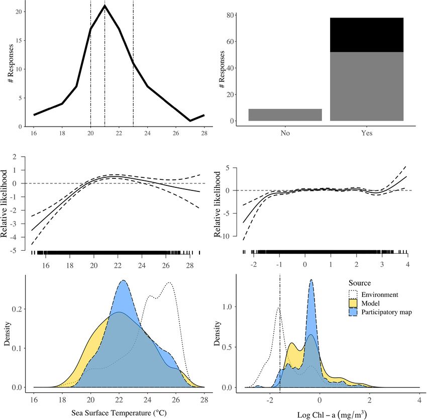
2 of 10                                                                                                                                           MASON ET AL.

                                                                                (b)
          (a)

                                                                                (c)

FIGURE 1      (a) Location of 1,644 gillnet sets with hammerheads present (circles) and 2,207 gillnet sets with hammerheads absent (plusses) used to build the
generalized additive model. Interview locations are indicated, and sets from the corresponding points shaded accordingly (darkest points indicate sets from
ports not interviewed). Dashed line indicates fishing grounds defined by a 2 buffer around all presence and absence points. (b) Distribution of fork length of
9,086 observed smooth hammerheads in gillnet sets between 2004 and 2016. Dashed line indicates estimated size at maturity. (c) Recorded mean monthly
landings (tons) recorded of smooth hammerhead sharks from January 1997, when Peru started recording disaggregated shark species landings, until
September 2013 (Adapted from de la Puente Jeri, 2013)

the third most commonly caught shark species in Peru and                           Endangered Species (CITES). Better understanding of the
the most commonly caught in the drift gillnet fishery that                         distribution and environmental niche of juvenile hammer-
operates out of northern ports (Figure 1a) (Gonzalez-Pestana                       head sharks would contribute to regional knowledge of this
et al., 2014), with total annual landings of approximately                         species and inform fisheries management.
500 tons (de la Puente Jeri, 2013). While legally defined as                           Species distribution models, which correlate documented
“small-scale” based on vessel size and operation with man-                         presences and, if available, absences of species with environ-
ual labor, these fisheries operate on a scale comparable to                        mental predictor variables, have been suggested as a valu-
industrial fisheries, with over 100,000 km of nets in the                          able tool for conservation decision-making (Guisan et al.,
water annually and fishing trips lasting up to 3 weeks                             2013). For smooth hammerheads in Peru, identifying envi-
(Alfaro-Shigueto et al., 2010). Nearly 18,000 small-scale                          ronmental characteristics of nursery areas and spatial zones
vessels reportedly operate along the 2,400 km coast,                               of high catch might inform management at finer spatial
employing over 67,000 fishers (Guevara-Carrasco & Ber-                             and/or temporal scales than landings data. However, species
trand, 2017).                                                                      distribution models are data-intensive, especially when inte-
     Landings of smooth hammerheads in Peru are almost                             grating multiple models as ensembles as is sometimes
entirely juveniles (Figure 1b), theorized to be due to overlap                     recommended (Araújo & New, 2007; Scales et al., 2017).
between fishing grounds and coastal nursery areas                                  The costs of collecting spatially explicit species data may be
(Castañeda, 2001; Gonzalez-Pestana, 2014). Seasonal pat-                           prohibitive for poorly studied species in remote areas.
terns in official landings data (Figure 1c) suggest that female                        One potential solution is incorporating local ecological
sharks approach coastal areas for parturition in the early aus-                    knowledge throughout the planning process (Anadón, Gimé-
tral summer (November and December), and juveniles                                 nez, Ballestar, & Pérez, 2009; Bélisle, Asselin, Leblanc, &
aggregate along the coast for several months before migrat-                        Gauthier, 2018; Folke, 2004). In addition to filling data
ing out for an oceanic adulthood (Compagno, 1984; Simp-                            gaps, incorporating local knowledge in ecological models
fendorfer, 2005). These landings data do not precisely reflect                     can legitimize management decisions and empower commu-
where sharks are caught given fishers' highly mobile behav-                        nities in resource management (Bélisle et al., 2018). Local
ior, but currently inform management decisions, including a                        ecological knowledge has been variously defined (Davis &
seasonal fishing ban implemented in 2016 to protect juvenile                       Ruddle, 2010); here we take the more experiential version of
hammerheads (IMARPE, 2014; PRODUCE, 2016) follow-                                  “place-based empirical knowledge” (Bélisle et al., 2018).
ing the 2013 listing of three hammerhead species under                             Increasingly called for in fisheries research and management,
Appendix II of the Convention on the International Trade of                        fishers' local ecological knowledge has been used to extend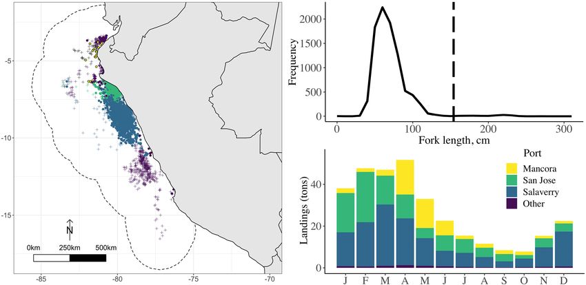
MASON ET AL.                                                                                                               3 of 10

scientific time-series, refine stock assessments, design          151.33 cm for males and 156.73 cm for females based on
marine protected areas, and provide valuable social insight       estimates for smooth hammerheads in the Gulf of California
for informing management (Aswani, 2018; Hind, 2014;               (Nava & Márquez-Farías, 2014). We classified each net set
Johannes, Freeman, & Hamilton, 2000; Neis, 1992; Sáenz-           by the presence or absence of juvenile hammerhead sharks.
Arroyo, Roberts, Torre, Cariño-Olvera, & Enríquez-                We omitted any sets for which latitude, longitude, or date
Andrade, 2005). Ecological modeling and studies of fishers'       data were missing, and sets from 38 trips for which
knowledge often examine similar spatial questions, yet            observers did not measure hammerheads in any sets but
rarely are the results compared or integrated. While a few        reported hammerhead capture for the trip.
studies have incorporated local knowledge with ecological
models, applications to marine environments and fisheries         2.2 | Biophysical model
are limited (Bélisle et al., 2018; Grant & Berkes, 2007;
                                                                  To determine juvenile hammerhead shark distribution and
Zhang & Vincent, 2017). In particular, studies with both
                                                                  probability of presence, we built generalized additive models
spatially explicit biophysical models and fishers' ecological
                                                                  (GAMs) with a binomial distribution with the package mgcv
knowledge have not been conducted for fisheries applica-
                                                                  (version 1.8.22) in R (version 3.4.2). We tested 17 predictor
tions. Examining fishers' knowledge alongside ecological
                                                                  variables based on previously published studies of juvenile
models could be a valuable way to understand and manage
                                                                  shark habitat (Alfaro-Shigueto, 2014; Campos, 2014;
data-poor small-scale fisheries, and holds potential for elas-
                                                                  Cartamil et al., 2010; Oh, Sequeira, Meekan, Ruppert, &
mobranch conservation globally.
                                                                  Meeuwig, 2017). These predictors included spatial variables:
     Peru's hammerhead shark fishery provides a unique
                                                                  latitude, longitude, distance to coast (m), distance to pro-
opportunity to incorporate fishers' knowledge with a spa-
                                                                  tected coastal islands (m), distance to river mouths
tially explicit onboard observer dataset spanning over a
                                                                  (m) (distances calculated with the R package geosphere ver-
decade. Collected by trained observers at a Peruvian conser-
                                                                  sion 1.5.7), and depth (m; from GEBCO bathymetry data);
vation nonprofit, these may be the only spatially explicit data
                                                                  temporal variables as factors: year and month; variables
on this species for this region. Furthermore, the high mobil-
                                                                  regarding fishing behavior: port of departure (n = 13),
ity and broad spatial scale of this fishery make the coarse
                                                                  whether the trip explicitly targeted sharks (binomial yes or
spatiotemporal resolution of local knowledge studies more
                                                                  no), and net mesh size (cm); satellite-derived environmental
appropriate (Zhang & Vincent, 2017). The goal of our study
                                                                  variables downloaded from Southwest Fisheries Science
is to examine the distribution of juvenile smooth hammer-
                                                                  Center Environmental Research Division's ERDDAP
head shark habitat along the Peruvian coast. We use two
                                                                  (Simons, 2017): log-transformed chlorophyll-a concentration
approaches: a statistical biophysical model and semistruc-
                                                                  (chl-a, mg/m3, 8 day composites from SeaWifs, MODIS,
tured interviews eliciting fishers' ecological knowledge.
                                                                  and VIIRS), sea surface temperature (SST) mean and SD
                                                                  ( C, from Pathfinder, MUR, and GHRSST); and mesoscale
2 | METHODS                                                       environmental variables downloaded from Aviso+ and the
                                                                  Copernicus Marine Environment Monitoring Service: sea
                                                                  level anomaly (SLA, m), finite-size Lyapunov exponents
2.1 | Fisheries data
                                                                  (FSLE, per day), and FSLE direction (theta,  ). Log chl-a
Onboard fishery observers recorded drift gillnet catch com-       outliers less than −10 mg/m3 were removed. We used a cor-
position and fishing location from 2000 to 2016 across 13        relogram correlation matrix to evaluate collinearity between
of latitude (16.53 –3.37 S). Observers used Global Position-    variables and in cases where correlation >0.6 we built
ing System (GPS) devices to record the location of each net       models for each correlated variable and dropped the variable
set at the onset of net deploy, end of net deploy, start of net   that yielded a poorer Akaike's Information Criterion (AIC).
retrieval, and end of net retrieval; we used the coordinates at        Following exploratory tests, we considered five candi-
the onset of net deploy in this study. Observers also recorded    date models: all uncorrelated variables, only static variables,
the main objective species for each fishing trip, port of         static and broad scale dynamic variables, static and meso-
departure and entry, and net dimensions. Observers identi-        scale dynamic variables, and only dynamic variables (model
fied animals to the species level with onboard guides and,        details in Table S2). We selected the final model based on
conditions permitting, recorded sex, maturity (clasper state),    percent deviance explained and AIC, as well as area under
and length (fork length or total length) of elasmobranchs.        curve (AUC) (Delong, Delong, & Clarke-Pearson, 1988),
Observers more frequently recorded fork length than total         and true skill statistic (TSS) (Allouche, Tsoar, & Kadmon,
length, so we converted all lengths to fork lengths (cm) with     2006) performance metrics with the R package ROCR (ver-
the conversion total length/1.28 for males and (total length +    sion 1.0.7). For AUC and TSS we took the average of five
 0.616)/2.18 for females, which was derived from larger           model iterations, with iterations trained on a random 75%
hammerheads (>1 m) in the Atlantic Ocean (Mas, Forsel-            subset of the data and tested with the remaining 25%. We
ledo, & Domingo, 2014). Fork length at maturity is                evaluated the contribution of each individual variable to the
4 of 10 MASON ET AL.
best model by fitting models with each single explanatory know if hammerheads are in the water?” After recording
variable, and then fitting the best model with each individual responses to this open question, the interviewer asked specif-
variable removed (Friedlaender et al., 2016), and comparing ically about environmental cues corresponding to variables
AIC values and percent deviance explained. We tested for used in the biophysical model including temperature, color
spatial autocorrelation in model residuals with Moran's of the water, currents or waves, distance from the coast, and
I statistics with R packages ncf (version 1.2.5) and spdep distance from coastal islands if the respondent had not
(version 0.7.8) (Dormann et al., 2007). mentioned them.
We used the final best model to predict hammerhead
shark presence likelihood, which we used as a measure of 2.4 | Interview analysis
habitat suitability, off the Peruvian coast. We predicted on
environmental data from 2012, an example year which was We digitized and georeferenced participatory maps in ArcGIS
an El Niño-Southern Oscillation “neutral” year, in the ArcMap following Wahle and D'Iorio (2010) and Levine and
months respondents identified as the hammerhead fishing Feinholz (2015). We categorized the polygons that respon-
season (December–April). We interpolated all covariates to dents had indicated as their hammerhead fishing grounds
a 0.25 grid to match the resolution at which SLA was based on which fishing months the respondent had specified
available. and collated all responses onto the same 0.25 grid for each
month (matching the biophysical model prediction grid),
where any part of a polygon intersecting a grid cell marked a
2.3 | Interviews
count. To characterize the environmental profile of these indi-
We conducted 87 semistructured interviews between cated fishing grounds, we overlaid the participatory grids with
February 8 and March 11, 2018 in the three ports with the the same monthly biophysical predictor rasters, selecting only
largest drift-gillnet fleets: San José (n = 32; 109 total ves- temperature and chl-a as they emerged as important in the
sels), Salaverry (n = 26; 70 total vessels), and Máncora interviews. From these rasters, we extracted environmental
(n = 29; 55 total vessels) (Alfaro-Shigueto, 2014) values, weighted by the number of polygons intersecting each
(Figure 1a). We specifically interviewed drift-gillnet captains grid cell. We hereafter refer to these distributions of values as
or boat owners as experts who make decisions about where the “fisher-mapped” hammerhead habitat.
and when to fish; sampling was opportunistic and based on We coded the interviews for emergent themes in NVivo
fishers' availability. Two of our respondents were not cur- (QSR International, version 12) and extracted any quantitative
rently active gillnetters, and it is possible that some inter- environmental information, hereafter referred to as the “fisher-
views were with the captains and owners of the same vessel, stated” hammerhead habitat. Only unprompted responses were
so our samples were not exact proportions of Alfaro-Shigue- used to characterize general patterns in hammerhead fishing
to's (2014) above estimates of vessel numbers. Interviews behavior, while prompted responses were also included for
were conducted in Spanish and translated into English prior subsequent qualitative and quantitative analysis of specific
to analysis. The interview protocol was approved by Stan- environmental cues. One such cue was temperature, for which
ford University's Institutional Review Board for human sub- we examined the distribution of fisher-stated temperature pref-
jects research on January 11, 2018, protocol #44763. erences from both prompted and unprompted responses. We
The interviewer first asked respondents demographic categorized the distribution into quantiles: we classified “opti-
questions about their fishing experience and methods, mal” habitat as the mean reported temperature ± 0.5 , second
including which months they most fish for hammerheads. most optimal as between the 0.25 or 0.75 quantiles and opti-
The interviewer then conducted a participatory mapping mal temperature, and 0.75 quantiles as least opti-
exercise to characterize the spatial extent of juvenile ham- mal. We interpreted responses about color of water as
merhead fishing grounds. This was done by asking respon- pertaining to chl-a concentration, as measures of turbidity or
dents to draw on a printed map where they catch other processes that may affect water color were less readily
hammerheads. The map was labeled with a longitude and available. We used a cutoff of 0.2 chl-a (mg/m3), or approxi-
latitude grid at the degree scale, the names of major ports, mately −1.6 log chl-a (mg/m3), which has been used to delin-
coastal islands, and the 250 m isobath representing the conti- eate oligotrophic from productive water masses in the north
nental shelf (see Figure S1, for example maps). Most fishers Pacific Ocean (Polovina, Howell, Kobayashi, & Seki, 2001)
were familiar with maps and coordinates, but if they seemed to differentiate between “blue” (i.e., clear) and “green”
unfamiliar the interviewer oriented them to the coast, their (i.e., colored, turbid) water.
home port, and the islands.
The interviewer also asked a series of questions to char-
2.5 | Biophysical model and interview comparisons
acterize fishers' environmental niche. Respondents were first
asked, “When you're fishing, what do you look for to know We employed two approaches to compare hammerhead
if there are hammerheads?” If needed, the interviewer clari- shark habitat suitability between the biophysical model pre-
fied with the terms “indicators,” “evidence,” or “how do you dictions and the fishers' knowledge. First, we qualitativelyMASON ET AL. 5 of 10
compared the spatial extent of hammerhead habitat from the TABLE 1 Contribution of each variable to the best biophysical model
biophysical model predictions, fisher-stated habitat, and par- deviance explained with individual variable model (Dev. explained, single),
full—1 model (Dev. explained, drop), and the difference in deviance
ticipatory maps. To visualize fisher-stated habitat spatially, explained between the full model and full-1 model (Difference from full)
we classified the same monthly rasters used in the biophysi-
Dev. explained, Dev. Difference
cal model prediction according to the optimal categories and Variable single explained, drop from full
cutoffs described above. Second, we compared the environ- Port 7.45 23.41 −8.52
mental profiles of predicted hammerhead habitat from the SST 4.75 23.56 −8.36
different methods. To compare biophysical model predic- Target 8.42 25.33 −6.60
tions and the fisher-mapped environmental variables, we Distance to islands 4.02 25.35 −6.58
extracted environmental values from the same cells where Log chl-a 3.29 25.63 −6.30
model predicted hammerhead suitability values were >0.5. Year 1.74 25.66 −6.27
We also determined the “background” environmental profile SST SD 2.29 26.29 −5.64
for each month for the overall fishing grounds, defined as a FSLE 0.30 26.66 −5.27
polygon surrounding all observed set nets with a 2 buffer SLA 1.09 26.68 −5.25
(Figure 1a). We compared the density distributions of FSLE direction 0.33 26.68 −5.24
model-derived and fisher-mapped variables with biophysical Month 1.36 26.75 −5.17
model partial plot response curves and fisher-stated variables Mesh size 5.61 27.09 −4.83
where applicable. We performed both these comparisons for Note. FSLE: finite-size Lyapunov exponents; SST: sea surface temperature;
each month in the peak fishing season (December–April) as SLA: sea level anomaly.
well as for an aggregate over the peak season. In the spirit of
epistemological pluralism (Miller et al., 2008), we present missing environmental data removed, the final model
results from the biophysical model and the interviews side included 3,212 net sets. We removed latitude and longitude
by side rather than use one method as the standard by which as covariates because they resulted in extreme values at the
to evaluate the other. edges of our predictions.
The port of departure and SST emerged as the most
important explanatory variables in terms of lost deviance
3 | RE SUL TS explained when dropped from the model, and targeting of
sharks had the most explanatory power when considered
3.1 | Fisheries data independently (Table 1). The mesoscale variables (SLA and
FSLE) had only a minor effect in describing shark habitat.
A total of 3,851 net sets from 125 boats and 13 ports were
Spatial predictions of shark habitat suitability (as measured
used to build the biophysical models, which included 1,644
by presence likelihood) are closely associated with coastal
juvenile hammerhead presences and 2,207 absences temperature and log chl-a distributions (Figure 2a,e). The
(Figure 1a). Fork lengths of hammerhead sharks caught in SST response curve showed peak predicted habitat between
sets (n = 9,086 sharks) ranged between 11 and 274 cm, with 20 and 22 C (Figure 3c). The log chl-a response curve has
the majority between 50 and 80 cm (Figure 1b). Net sets an inflection point approaching 0 at −1.6 mg/m3
were primarily concentrated along the northern Peruvian (Figure 3d), further supporting our cutoff defining fisher-
coast. The majority of set data came from the port of Sala- stated “green water.” We did not find significant autocorrela-
verry (n = 2,101), followed by San José (n = 950), then tion spatial structure in the residuals (Moran's
Mancora (n = 84). Hammerhead shark landings varied I statistic = −3.13 × 10⁻⁴, standard deviate = −2.13,
between months, with the majority of landings occurring p = 0.98), justifying running a model without latitude and
from January to May. However, northern ports (notably longitude.
Mancora, 4.10 S) showed peak catches between April and
June (Figure 1c). 3.3 | Interviews
Respondents drew a total of 269 polygons spanning 17.42 of
3.2 | Biophysical model
latitude (0.22 –17.64 S) and 12.80 longitude (76.54 –
The best biophysical model was the full uncorrelated model 89.34 W) (Figure 2b,f). The highest overlap was 24 polygons
containing 12 variables, with 31.9% deviance explained (see in December, January, and February. Based on respondents'
Table S1 for model summary). This model had good predic- reports of the months they most fish for hammerheads, we
tive performance with an AUC of 0.83 and a TSS of 0.49 defined the peak fishing season for all ports as December
(see Table S2 for model selection statistics). This model through April.
included year, month, port of departure, targeting of sharks, Respondents' most common unprompted explanation of
mesh size, distance to islands, log chl-a, SST, SST SD, SLA, drivers of hammerhead fishing behavior was that fishers cue
FSLE, and FSLE direction as covariates; with points with to prey aggregations, such as anchovy, which they know6 of 10 MASON ET AL.
(a) (b) (c) (d)
(e) (f) (g) (h)
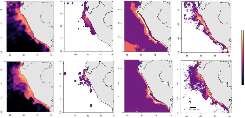
FIGURE 2 Median generalized additive model prediction (GAM) of juvenile hammerhead shark catch (a, e), aggregated participatory map polygons (b, f),
fisher-stated temperature niche (c, g), and fisher-stated ocean color niche (d, h) for January (top row) and April (bottom row), 2012. Habitat suitability in each
map goes from low (dark) to high (bright), measured as 0–1 presence likelihood for GAM predictions, 1–24 overlapping polygons for participatory maps,
three discrete categories based on fisher-stated temperature quantiles ( C, see Figure 3) for sea surface temperature, and −1.6 to 3.0 mg/m3 for log chl-a
attract sharks (30 respondents, 34%). The next most common and more northward footprint than the biophysical model
unprompted answer had to do with the color of the water: predictions. The fisher-mapped temperature distribution for
green, brown, turbid, dark (30%). Eighteen percent of the peak fishing season (Figure 3e) had a warmer peak
respondents explained that they share fishing information (mean [SD] = 22.74 C [1.62]) than fisher-stated temperature
via radio communication, including providing specific coor- (Figure 3a) (mean [SD] = 21.36 C, [2.29]), which showed a
dinates, in social networks that may bridge ports. Fifteen similar pattern to the biophysical model partial plot relation-
percent described a “trial and error” strategy, emphasizing ship of SST (Figure 3c) (peak ~20–22 C). The distributions
that with gillnets, the catch can be a surprise. Including of SST from the biophysical model prediction (mean [SD] =
prompted responses, 74% of respondents use temperature to 22.32 C [1.97]) and fisher-mapped values are more similar
fish for hammerheads, usually specifying warmer waters, to each other and distinct from the background environmen-
and 48% (42) gave a specific degree or range; these specific tal signal (mean [SD] = 24.05 C [1.83]) (Figure 3e). The
responses comprise our fisher-stated hammerhead habitat temperature distributions of biophysical model predictions
temperature distribution (Figure 3a). Ninety percent of tend toward the warmer quantiles of fisher-stated tempera-
respondents use dark, turbid, or greenish waters to locate ture in later months, with the most overlap in January and
hammerheads (Figure 3b), and two respondents noted a rela- the least in December (Figure S2). During the peak fishing
tionship between warmer and greener water. Some respon- season, the model prediction and fisher-mapped log chl-a
dents also noted when prompted that hammerheads are distributions had similar peaks (model mean [SD] = −0.41
closer to the coast in the summer than in the winter, but in mg/m3 [0.73]; maps mean [SD] = −0.46 mg/m3 [0.62])
general did not cue to this distance or the other prompted higher than background log chl-a (mean [SD] = −1.29
variables as much as those described above. In subsequent mg/m3 [0.81]) (Figure 3f), again with least overlap in
results and discussion of fishers' knowledge, we focus on December (Figure S2).
temperature and chl-a as they were the most commonly
reported environmental drivers of fishing behavior.
4 | DISCUSSION
3.4 | Biophysical model and interview comparisons This study is one of the first to assess the complementarity
The spatial distributions of fisher-stated environmental vari- of fishers' knowledge and biophysical models in describing
ables, participatory maps, and biophysical model predictions catch patterns, lending further credence to the utility of fish-
all follow similar patterns, with highest predicted habitat ers' knowledge for conservation planning in data-poor situa-
close to shore, particularly the coastal waters off San José tions. The convergence of results across three methods
(Figure 2). The participatory maps tended to have a smaller (biophysical model, fishers' maps, and fishers' descriptionsMASON ET AL. 7 of 10
(a) (b)
(c) (d)
(e) (f)
FIGURE 3 Model and interview comparison of sea surface temperature (a, c, e) and log chlorophyll-a (b, d, f) distributions, including fisher-stated variables
(a, b), biophysical model partial plots (c, d), and density distributions (e, f) of fisher-mapped variables (dashed line), biophysical model prediction values >0.5
(solid line), and background environment (dotted line) for the peak fishing season (December–April) 2012. For fisher-stated temperature (a), vertical dashed
lines indicate quartiles used to categorize “optimal” habitat in Figure 2. For fisher-stated chlorophyll (b), we show the number of respondents that did (yes)
and did not (no) indicate that they use the color of the water to fish hammerheads, with prompted responses in black and unprompted in gray. Vertical dashed
line in (f) indicates −1.6 cutoff representing green water
of their environmental niche) is encouraging for bringing potential for incorporating more dynamic approaches
together these different sources of knowledge. The dynamic (Alfaro-Shigueto, Mangel, Dutton, Seminoff, & Godley, 2012;
nature of juvenile hammerhead shark habitat shown here Hazen et al., 2018; Howell, Kobayashi, Parker, Balazs, &
suggests that including sea surface temperature and Polovina, 2008).
chlorophyll-a patterns in conservation planning may allow Both our model and respondents' accounts of how they
fishers and conservation practitioners to refine spatiotempo- use environmental variables emphasized temperature, with
ral management approaches for these sharks, with the fishers also cuing to color of water, which may refer to a8 of 10 MASON ET AL.
complex combination of productivity, turbidity, and fronts; respondents tended to speak in recent terms. There was also
these results are broadly similar to other published studies of potential sampling bias in that we could only talk to fishers
juvenile shark habitat (Cartamil et al., 2010; Oh et al., who were in port, so the fishers at sea for the duration of the
2017). Aggregations of prey fish, which fishers emphasized interviews may utilize different fishing strategies. However,
in their fishing strategies, are also linked to these productive as we covered between ~30 and ~50% of drift-gillnet cap-
oceanographic conditions (Polovina et al., 2001). Mesoscale tains in these ports and reached general convergence in
covariates, including FSLE and SLA, which are often prox- responses, this bias may be negligible.
ies for productive feeding areas, did not have a large effect Our methods of combining fishers' knowledge and a bio-
in predicting hammerhead habitat. Similarly, fishers did not physical model could be improved with future research to
emphasize currents or waves in their environmental elicit the multivariate relationships in fishers' environmental
responses. These mesoscale covariates may not be effective niche, rather than comparing single variable distillations to
predictors for juvenile sharks within their nursery grounds, the multivariate model. Yet, the similarity between niche
and perhaps are more appropriate predictors for adult preda- maps based on temperature and chl-a and model predictions
tors (e.g., swordfish; Scales et al., 2018). Some fisher is encouraging on its own, as many aspects of fishers'
responses pertained to optimal fishing practices broadly, not decision-making are complex and not easily quantified. Fur-
just for targeting hammerheads. For example, a few respon- ther work integrating fishers' knowledge and biophysical
dents explained that dark and turbid water obscures their models would be particularly useful for predicting condi-
nets, promoting catch of many species. Nevertheless, these tions under climate change and extreme climatic events
results show that both juvenile hammerheads and fishers including El Niño and La Niña. Species distribution models,
have a distinct niche separate from the background environ- as done here, are fit on observed environmental conditions
ment, even when fishers may be fishing by trial and error or and may not hold up to novel conditions as the environment
sharing information. changes (Franklin, 2010; Guisan & Thuiller, 2005). Iterative
In particular, the spatial and temporal variability of this work that incorporates fishers' understanding and percep-
catch vulnerability niche has implications for the 2016 ham- tions of these changing relationships to existing distribution
merhead fishing ban. The ban may not adequately protect models may be useful for updating them for changing condi-
juvenile hammerhead sharks near northern ports operating tions. Some respondents also reflected that they have had to
later in the season. Anomalous oceanographic years may adapt their knowledge to novel conditions; the methods they
also result in greater vulnerability outside of the closed sea- previously used no longer apply because there are too few
son (Hazen et al., 2018; Oliver et al., 2018). Further study of fish or because the environment has changed. This points to
the avenues for dynamic approaches and incorporating fish- the urgency of iterative work that further applies fishers'
ers' knowledge and perspectives may be a productive path- knowledge in what Bélisle et al. (2018) terms the instrumen-
way toward more effective management. Similarly, better tal, or empowering use: knowledge sharing platforms for sci-
understanding of smooth hammerhead population dynamics entific study may also be a valuable means of sharing
and ontogenetic niche separation might help ensure that knowledge among generations of fishers.
management measures protect appropriate life stages This study points to the utility of integrating local knowl-
(Kinney & Simpfendorfer, 2009). edge and biophysical modeling for conservation and man-
From an epistemological standpoint, where the two agement of the hammerhead shark fishery in Peru. It also
methods diverge may highlight biases in either approach. shows promise for other data-poor fisheries where spatially
The biophysical model leaves the majority of the deviance explicit data is limited, absent, or difficult to obtain. Inter-
unexplained, which may be due to social factors or individ- viewing fishers or other resource users may provide suffi-
ual variability in fishing cues. Because the observer dataset cient information for prioritizing research and implementing
included several projects with different objectives, observer conservation planning in data-poor systems. In addition,
coverage for ports is not necessarily representative of the fishers' knowledge may prove useful as a component of
entire population of fishers. In particular, the observer data- ensemble modeling efforts. These findings may encourage
set has disproportionately fewer records from Máncora than use the of fishers' knowledge in Peru and elsewhere to
our interview dataset and from the overall hammerhead fish- inform conservation decision-making for data-poor fisheries.
ery, and greater representation of more southern ports. This
bias may explain the overall more northern and warmer pat-
terns from fishers' knowledge than the biophysical model ACKNOWLEDGMENTS
predictions. Fishers' knowledge may also vary based on age, Deepest thanks to D. Sarmiento Burien, B. Diaz Solano,
experience, port, and other factors, but these were not exam- G. Vela, and participating fishermen for sharing their knowl-
ined here. The implementation of the hammerhead fishing edge and time. We thank A. Gonzalez-Pestana, A. Pásara
ban in 2016 may have altered fishing behavior, and although Polack, N. Acuña, and F. Córdova for input on the interview
we asked questions specifying conditions before the ban, protocol, S. de la Puente Jeri for assistance with landingsMASON ET AL. 9 of 10
data, and J. Selgrath, H. Blondin, and R. Carlson for advice Cartamil, D., Wegner, N. C., Kacev, D., Ben-Aderet, N., Kohin, S., &
Graham, J. B. (2010). Movement patterns and nursery habitat of juvenile
on analyzing the participatory maps. J.G.M. thanks the NF thresher sharks Alopias vulpinus in the Southern California bight. Marine
Nereus Program, ARCS Foundation, and SCB for support. Ecology Progress Series, 404, 249–258. https://doi.org/10.3354/meps08495
Castañeda, J. (2001). Biologia y Pesqueria del ‘Tiburón Martillo’ (Sphyrna
zygaena) en Lambayeque, 1991-2000. Informe Progresivo Instituto del Mar
del Peru, 139, 17–32.
CONFLICTS OF IN TER EST Compagno, L. J. V. (1984). FAO Species Catalogue. In Sharks of the world: An
The authors declare no conflicts of interest. annotated and illustrated catalogue of shark species known to date.” FAO
Fisheries Synopsis No. 125 4 (Part 2) (Vol. 4, pp. 521–532). Rome, Italy:
Food and Agriculture Organization of the United Nations. https://doi.org/10.
1016/S0921-4526(05)00705-2
DATA ACCESSIBILITY Davis, A., & Ruddle, K. (2010). Constructing confidence: Rational skepticism
and systematic enquiry in local ecological knowledge research. Ecological
Interview protocols and full transcript data are available at Applications, 20(3), 880–894. https://doi.org/10.1890/09-0422.1
https://purl.stanford.edu/wv848yd6100. de la Puente Jeri, S. (2013). Diagnóstico Situacional del Género Sphyrna en el
Perú, con Especial Énfasis en el ‘Tiburón Martillo’ Sphyrna zygaena
(Linnaeus, 1758). Lima, Perú: Consultoría Realizada para la Dirección Gen-
eral de Diversidad Biológia, Ministerio del Ambiente.
Author contributions
Delong, E. R., Delong, D. M., & Clarke-Pearson, D. L. (1988). Comparing the
J.G.M. conducted the interviews, performed the analysis, areas under two or more correlated receiver operating characteristic curves:
A nonparametric approach. Biometrics, 44(3), 137–845.
and wrote the paper. J.A.-S. and J.C.M. designed and Dormann, C. F., McPherson, J. M., Araújo, M. B., Bivand, R., Bolliger, J.,
directed onboard observer data collection, provided access to Carl, G., … Kühn, I. (2007). Methods to account for spatial autocorrelation
fishermen, and identified hammerheads as a research prior- in the analysis of species distributional data: A review. Ecography, 30(5),
609–628. https://doi.org/10.1111/j.2007.0906-7590.05171.x
ity. E.L.H., S.J.B., and S.B. contributed to the biophysical
Dulvy, N. K., Fowler, S. L., Musick, J. A., Cavanagh, R. D., Kyne, P. M.,
model analysis and critical revision of the manuscript. Harrison, L. R., … Pollock, C. M. (2014). Extinction risk and conservation
L.B.C. contributed to critical revision of the manuscript. of the World's sharks and rays. eLife, 3, e00590. https://doi.org/10.7554/
eLife.00590
Folke, C. (2004). Traditional knowledge in social-ecological systems. Ecology
ORCID and Society, 9(3), 5–9. Retrieved from http://www.ecologyandsociety.
org/vol9/iss3/art7/
Julia G. Mason https://orcid.org/0000-0002-8828-353X Franklin, J. (2010). Moving beyond static species distribution models in support
of conservation biogeography. Diversity and Distributions, 16(3), 321–330.
https://doi.org/10.1111/j.1472-4642.2010.00641.x
REFERENC ES Friedlaender, A. S., Hazen, E. L., Goldbogen, J. A., Stimpert, A. K.,
Alfaro-Shigueto, J. (2014). Servicio de Consultoría Para El Levantamiento de Calambokidis, J., & Southall, B. L. (2016). Prey-mediated behavioral
Información de La Pesca de Tiburones En La Zona Norte Del País.” Informe responses of feeding blue whales in controlled sound exposure experiments
Final de Consultoría Nr. 058-2014-MINAM-OGA. Lima, Peru: Ministerio mediated behavioral responses of feeding blue whales in controlled sound
del Ambiente. exposure experiments. Ecological Applications, 26(4), 1075–1085. https://
Alfaro-Shigueto, J., Mangel, J. C., Dutton, P. H., Seminoff, J. A., & doi.org/10.1002/15-0783
Godley, B. J. (2012). Trading information for conservation: A novel use of Gonzalez-Pestana, Adriana. 2014. “Trophic level and nursery areas for juvenile
radio broadcasting to reduce sea turtle bycatch. Oryx, 46(3), 332–339. S. zygaena in Northern Peru.” Universidad Científica del Sur.
https://doi.org/10.1017/S0030605312000105 Gonzalez-Pestana, A., Kouri, C. J., & Velez-Zuazo, X. (2014). Shark Fisheries
Alfaro-Shigueto, J., Mangel, J. C., Pajuelo, M., Dutton, P. H., Seminoff, J. A., & in the Southeast Pacific: A 61-Year Analysis from Peru. F1000Research, 3,
Godley, B. J. (2010). Where small can have a large impact: Structure and 1–19. https://doi.org/10.12688/f1000research.4412.1
characterization of small-scale fisheries in Peru. Fisheries Research, 106(1), Grant, S., & Berkes, F. (2007). Fisher knowledge as expert system: A case from
8–17. https://doi.org/10.1016/j.fishres.2010.06.004 the longline fishery of Grenada, the Eastern Caribbean. Fisheries Research,
Allouche, O., Tsoar, A., & Kadmon, R. (2006). Assessing the accuracy of spe- 84, 162–170. https://doi.org/10.1016/j.fishres.2006.10.012
cies distribution models: Prevalence, kappa and the true skill statistic (TSS). Guevara-Carrasco, R., & Bertrand, A. (2017). Atlas de La Pesca Artesanal Del
Journal of Applied Ecology, 43(6), 1223–1232. https://doi.org/10.1111/j. Mar Del Perú (p. 183). Lima, Perú: Edición IMARPE-IRD.
1365-2664.2006.01214.x Guisan, A., & Thuiller, W. (2005). Predicting species distribution: Offering more
Anadón, J. D., Giménez, A., Ballestar, R., & Pérez, I. (2009). Evaluation of local than simple habitat models. Ecology Letters, 8(9), 993–1009. https://doi.
ecological knowledge as a method for collecting extensive data on animal org/10.1111/j.1461-0248.2005.00792.x
abundance. Conservation Biology, 23(3), 617–625. https://doi.org/10.1111/j. Guisan, A., Tingley, R., Baumgartner, J. B., Naujokaitis-Lewis, I.,
1523-1739.2008.01145.x Sutcliffe, P. R., Tulloch, A. I. T., … Martin, T. G. (2013). Predicting species
Araújo, M. B., & New, M. (2007). Ensemble forecasting of species distributions. distributions for conservation decisions. Ecology Letters, 16(12),
Trends in Ecology & Evolution, 22(1), 42–47. https://doi.org/10.1016/j.tree. 1424–1435. https://doi.org/10.1111/ele.12189
2006.09.010 Hazen, E. L., Scales, K. L., Maxwell, S. M., Briscoe, D. K., Welch, H.,
Aswani, S. (2018). Integrating indigenous ecological knowledge and customary Bograd, S. J., … Lewison, R. L. (2018). A dynamic ocean management tool
sea tenure with marine and social science for conservation of Bumphead Par- to reduce bycatch and support sustainable fisheries. Science Advances, 4(5),
rotfish (Bolbometopon muricatum) in the Roviana Lagoon, Solomon Islands. eaar3001. https://doi.org/10.1126/sciadv.aar3001
Environmental Conservation, 31(1), 69–83. https://doi.org/10.1017/ Hind, E. J. (2014). A review of the past, the present, and the future of fishers'
S037689290400116X knowledge research: A challenge to established fisheries science. ICES Jour-
Bélisle, A. C., Asselin, H., Leblanc, P., & Gauthier, S. (2018). Local knowledge nal of Marine Science, 72(2), 341–358. https://doi.org/10.1093/
in ecological modeling. Ecology and Society, 23(2), 14. https://doi.org/10. icesjms/fsu169
5751/ES-09949-230214 Hoffmann, M., Hilton-Taylor, C., Angulo, A., Böhm, M., Brooks, T. M.,
Campos, D. M. Z. (2014). Presencia de Neonatos de La Familia Sphyrnidae En Butchart, S. H. M., … Stuart, S. N. (2018). The impact of conservation on
Redes de Enmalle, Desembarcados En El Puerto El Triunfo. San Salvador, the status of the World's vertebrates. Science, 330(6010), 1503–1509. https://
El Salvador: Ciudad Universitaria. doi.org/10.1126/science.119444210 of 10 MASON ET AL.
Howell, E. A., Kobayashi, D. R., Parker, D. M., Balazs, G. H., & Polovina, J. J. fishers of the Gulf of California. Proceedings of the Royal Society B:
(2008). TurtleWatch: A tool to aid in the bycatch reduction of loggerhead Biological Sciences, 272(1575), 1957–1962. https://doi.org/10.1098/rspb.
turtles Caretta caretta in the Hawaii-based Pelagic longline fishery. Endan- 2005.3175
gered Species Research, 5(1987), 267–278. https://doi.org/10.3354/esr00096 Scales, K. L., Hazen, E. L., Jacox, M. G., Castruccio, F., Maxwell, S. M.,
IMARPE. (2014). Evaluacion Poblacional del Tiburon Martillo Sphyrna Lewison, R. L., & Bograd, S. J. (2018). Fisheries bycatch risk to marine
zygaena en el Mar Peruano Durante el Periodo 1996–2014 (p. 22). Lima, megafauna is intensified in Lagrangian coherent structures. Proceedings of
Peru: Area Funcional de Investigaciones en Biodiversidad Marina. the National Academy of Sciences, 115(28), 7362–7367.
Johannes, R. E., Freeman, M. M. R., & Hamilton, R. J. (2000). Ignore fishers' Scales, K. L., Schorr, G. S., Hazen, E. L., Bograd, S. J., Miller, P. I., Andrews, R. D.,
knowledge and miss the boat. Fish and Fisheries, 1, 257–271. … Falcone, E. A. (2017). Should I stay or should I go? Modelling year – round
Kinney, M. J., & Simpfendorfer, C. A. (2009). Reassessing the value of nursery habitat suitability and drivers of residency for fin whales in the California. Diver-
areas to shark conservation and management. Conservation Letters, 2, sity and Distributions, 23, 1204–1215. https://doi.org/10.1111/ddi.12611
53–60. https://doi.org/10.1111/j.1755-263X.2008.00046.x Simons, R. A. (2017). ERDDAP. Retrieved from https://coastwatch.pfeg.noaa.
Levine, A. S., & Feinholz, C. L. (2015). Participatory GIS to inform coral reef gov/erddap.
ecosystem management: Mapping human coastal and ocean uses in Hawaii. Simpfendorfer, C. (2005). Smooth Hammerhad Sphyrna zygaena (Linnaeus,
Applied Geography, 59, 60–69. https://doi.org/10.1016/J.APGEOG.2014. 1785). In S. L. Fowler, R. D. Cavanagh, M. Camhi, G. H. Burgess,
12.004 G. M. Cailliet, S. V. Fordham, et al. (Eds.), Sharks, rays and chimaeras: The
Mas, F., Forselledo, R., & Domingo, A. (2014). Length-length relationships for status of the Chondrichthyan fishes. Status survey (pp. 318–320). Gland,
six pelagic shark species commonly caught in the Southwestern Atlantic Switzerland and Cambridge, England: IUCN.
Ocean (Collected Volumes of Scientific Papers, ICCAT 70). Wahle, C., & D'Iorio, M. (2010). Mapping human uses of the oceans: Informing
Miller, T. R., Baird, T. D., Littlefield, C. M., Kofinas, G., Stuart Chapin, F., marine spatial planning through participatory GIS. Silver Spring, MD:
III, & Redman, C. L. (2008). Epistemological pluralism: Reorganizing inter- NOAA National Marine Protected Areas Center.
disciplinary research. Ecology and Society, 13(2), 46. Worm, B., Davis, B., Kettemer, L., Ward-Paige, C. A., Chapman, D.,
Nava, P. N., & Márquez-Farías, J. F. (2014). Talla de Madurez del Tiburón Mar- Heithaus, M. R., … Gruber, S. H. (2013). Global catches, exploitation rates,
tillo, Sphyrna zygaena, Capturado en el Golfo de California. Hidrobiológica, and rebuilding options for sharks. Marine Policy, 40(1), 194–204. https://
24(242), 129–135. doi.org/10.1016/j.marpol.2012.12.034
Neis, B. (1992). Fishers' ecological knowledge and stock assessment in New- Zhang, X., & Vincent, A. C. J. (2017). Integrating multiple datasets with species
foundland. Newfoundland and Labrador Studies, 8(2), 155–187. distribution models to inform conservation of the poorly-recorded Chinese
Oh, B. Z. L., Sequeira, A. M. M., Meekan, M. G., Ruppert, J. L. W., & seahorses. Biological Conservation, 211, 161–171. https://doi.org/10.1016/J.
Meeuwig, J. J. (2017). Predicting occurrence of juvenile shark habitat to BIOCON.2017.05.020
improve conservation planning. Conservation Biology, 31(3), 635–645.
https://doi.org/10.1111/cobi.12868 SUPPORTING I NFORMATION
Oliver, E. C. J., Donat, M. G., Burrows, M. T., Moore, P. J., Smale, D. A.,
Alexander, L. V., … Wernberg, T. (2018). Longer and more frequent marine Additional supporting information may be found online in
heatwaves over the past century. Nature Communications, 9(1324), 1–12. the Supporting Information section at the end of this article.
https://doi.org/10.1038/s41467-018-03732-9
Polovina, J. J., Howell, E., Kobayashi, D. R., & Seki, M. P. (2001). The transi-
tion zone chlorophyll front, a dynamic global feature defining migration and
How to cite this article: Mason JG, Alfaro-
forage habitat for marine resources. Progress in Oceanography, 49,
469–483. https://doi.org/10.1016/S0079-6611(01)00036-2 Shigueto J, Mangel JC, et al. Convergence of fishers'
PRODUCE. (2016). Establecen Temporada de Pesca del Recurso Tiburón Mar- knowledge with a species distribution model in a
tillo a Nivel Nacional. Lima, Peru: Resolución Ministerial N Peruvian shark fishery. Conservation Science and
008-2016-PRODUCE.
Sáenz-Arroyo, A., Roberts, C. M., Torre, J., Cariño-Olvera, M., & Enríquez-
Practice. 2019;e13. https://doi.org/10.1111/csp2.13
Andrade, R. R. (2005). Rapidly shifting environmental baselines amongYou can also read