A predictive internet based model for COVID 19 hospitalization census - Nature
←
→
Page content transcription
If your browser does not render page correctly, please read the page content below
www.nature.com/scientificreports
OPEN A predictive internet‑based model
for COVID‑19 hospitalization
census
Philip J. Turk1*, Thao P. Tran1,2, Geoffrey A. Rose1 & Andrew McWilliams1
The COVID-19 pandemic has strained hospital resources and necessitated the need for predictive
models to forecast patient care demands in order to allow for adequate staffing and resource
allocation. Recently, other studies have looked at associations between Google Trends data and the
number of COVID-19 cases. Expanding on this approach, we propose a vector error correction model
(VECM) for the number of COVID-19 patients in a healthcare system (Census) that incorporates Google
search term activity and healthcare chatbot scores. The VECM provided a good fit to Census and
very good forecasting performance as assessed by hypothesis tests and mean absolute percentage
prediction error. Although our study and model have limitations, we have conducted a broad and
insightful search for candidate Internet variables and employed rigorous statistical methods. We have
demonstrated the VECM can potentially be a valuable component to a COVID-19 surveillance program
in a healthcare system.
The SARS-CoV-2 coronavirus, initially emerging in Wuhan, China on December 2019, has spread worldwide
in what is now described as the COVID-19 pandemic. The coronavirus outbreak was declared a global public
health emergency1 by the World Health Organization [WHO] on January 30, 2020, and as of October 17, there
were over 39 million confirmed cases worldwide with over a million lives lost2. While evidence supports the
effectiveness of guidelines and r estrictions3,4 in containing the spread of SARS-CoV-2 (“flattening the curve”),
the health and economic consequences have been devastating on many l evels5,6.
By April 11, 2020, the US had more COVID-19 cases and deaths than any other c ountry2. As of June 30,
the US had 4% of the world’s population, but 25% of its coronavirus cases. While most states avoided a rapid
surge in cases during the first phase of the pandemic, the majority of them have begun to lift social distancing
and gathering restrictions, raising concern that we will see large surges in infection incidence and m ortality7–9.
Without a widely available vaccine, we expect that the pandemic activity will continue to rise and fall through
the winter, requiring health care systems to remain vigilant as they balance hospital resources.
As has been seen in this pandemic, when SARS-CoV-2 prevalence grows quickly and reaches high levels in
a community, large numbers of people develop symptomatic COVID-19 infection. Many require hospitaliza-
tion, and this has the capacity to overwhelm regional health care resources (e.g., Northern Italy and New York).
Acknowledging this risk, health care systems have implemented crisis planning to guide infection management,
bed capacity, and secure vital supplies (e.g., ventilators and personal protective equipment)10–12. Ideally, health
systems’ efforts to best prepare for COVID-19 demand surges would be informed by data that provide early
warning, or “lead time”, on the local prevalence and impact of COVID-19.
Traditional epidemiological models (e.g., SIR model) do not provide health system leaders with lead time for
accurate planning. In searching for leading indicators, researchers have turned to internet data that reflect trends
in community behaviors and activity. In recent years, researchers in the field of infodemiology13 have utilized
various internet search data to predict different health-related metrics, such as dengue incidence14, infectious
disease risk c ommunication15, influenza epidemic m onitoring16, and malaria s urveillance17. Google Trends is one
of the most popular tools that allows researchers to pull search query data of a random, representative sample
drawn from billions of daily searches on Google-associated search e ngines18.
In the last six months, several papers have made use of Google Trends data to test the association between
the popularity of certain coronavirus-related terms and the number of cases and deaths related to COVID-
1919–22. While these papers do not address using Google Trends data to build a predictive model for COVID-19
modeling applications21,23, they have contributed to our collective understanding of the relationship between
1
Center for Outcomes Research and Evaluation, Atrium Health, Charlotte, NC 28204, USA. 2Psychology
Department, Colorado State University, Fort Collins, CO 80523, USA. *email: Philip.Turk@atriumhealth.org
Scientific Reports | (2021) 11:5106 | https://doi.org/10.1038/s41598-021-84091-2 1
Vol.:(0123456789)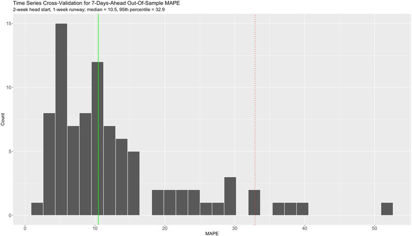
www.nature.com/scientificreports/
covid coronavirus
symptoms covid covid testing + covid test + covid19 Testing + covid19 test + covid 19 Testing + covid 19 test
fever + chills headache
“shortness of breath” “shortness of breath” + “trouble breathing” + “difficulty breathing”
tired + fatigue pneumonia
“sore throat” + cough CDC
Table 1. Google Trends search terms used. Google Trends search terms with no punctuation will contain the
term(s), along with other words, in any order. Using double quotation marks give results that include that exact
term, possibly with words before and after. The use of a plus sign ( +) is shorthand for OR.
the public’s internet search behavior and the pandemic, supporting the notion that search query data can be
used for surveillance purposes.
In addition to internet users’ search query data, another source of data that is of importance for public health
research is geospatial mobility data. Since the initial outbreak of COVID-19 in Wuhan, China, researchers
have believed that population mobility is a major driver of the exponential growth in the number of infected
cases24–26. It is now well-accepted that mobility reduction and social distancing are timely and effective meas-
ures to attenuate the transmission of COVID-1927,28. Thus, it stands to reason that mobility changes may be a
predictor of COVID-19 hospital case volume. Many different interactive dashboards are available and display
up-to-date regional mobility data that are publicly available, most notably from Facebook and Apple Maps29–33.
In this paper, we specifically considered Apple Mobility Trend Reports and Facebook Movement Range Maps,
which are mobility data reported in the form of aggregated, privacy-protected information.
Another area with great potential in modeling COVID-19 hospital case volume are the data generated by vir-
tual AI-based triage systems (also known as “healthcare chatbots”). During the COVID pandemic, these chatbots
have been deployed to provide virtual consultation to people who are concerned they may have SARS-CoV-234,35.
rganizations36. Medical content, together with
In particular, Microsoft offers its Health Bot service to healthcare o
an interactive symptom checker, custom conversational flow, and a system of digital personal assistants can be
integrated into the Health Bot configuration to help screen people for potential coronavirus infection through
a risk assessment37–40. User outcomes (with no personally identifiable information) can be aggregated, and the
number of people “flagged” with COVID-19 could then be potentially used to predict COVID-19 hospital case
volume in the future. Specifically, if a hospital has its own Health Bot for delivering a tele-health COVID-19 risk
assessment to the public, then it is reasonable to expect that people who are identified as having COVID-19 are
likely to seek treatment from the same hospital.
Atrium Health is a healthcare system operating across North Carolina, South Carolina, and Georgia, with
the majority of its hospitals located in the greater Charlotte metropolitan area. Investigators from the Atrium
Health Center for Outcomes Research and Evaluation sought to leverage internet search term volumes, mobility
data, and Health Bot risk assessment counts, collectively known as “Internet variables”, to provide leadership
with information that would allow for planning purposes during the COVID-19 pandemic. Specifically, this
paper describes the steps to characterize and understand the relationships between our Internet variables and
the daily total number of COVID-19 patients hospitalized in our hospital system’s primary market. Furthermore,
we sought to develop a novel forecast model for these patients to provide advance warning of any anticipated
surges in patient care demands.
Methods
Measures. Our interest lies in the population served by Atrium Health’s greater Charlotte market area which
spans approximately 11 counties in western North Carolina and two counties in northern South Carolina. This
area includes approximately 400,000 South Carolina residents, 2.5 million North Carolina residents (24% of the
North Carolina population), over 1.1 million of which live in Mecklenburg County and 900,000 within North
Carolina’s largest city, Charlotte41.
Because of the focus on health care system capacity, our outcome variable of interest is the total COVID-19
positive census across 11 Atrium Health Hospitals that serve the greater Charlotte market (hereafter referred
to as “Census”) with an additional virtual hospital, Atrium Health Hospital at Home, providing hospital level
care in a patient’s home. Census is a cross-sectional count taken each morning as the total number of patients
hospitalized and COVID-19 positive.
Rather than a raw count of “hits”, Google Trends data reflect the relative popularity of a search term, or rela-
tive search volume (RSV). Specifically, the RSV of a search term is calculated as the proportion of interest in
that particular topic relative to all searches over a specified time range and location. The RSV is normalized to
a scale of 0–100. “0” indicates that the term appears in very few searches and “100” shows maximum interest
in the term for the chosen time range and r egion18. To retrieve Google Trends data for our analysis, we utilized
the gtrendsR package in R (https://cran.r-project.org/web/packages/gtrendsR/gtrendsR.pdf). We performed
twelve different queries from 02/21/20 to 08/01/20 for Google Trends’ “Charlotte NC” metro designation (county-
level data is unavailable) using a list of terms obtained based on our prior beliefs and the medical expertise of
our physicians. Since punctuations can influence the search results42,43, we followed the guidelines from Google
News Initiative44 to refine our search queries. Details on the search terms can be found in Table 1.
Scientific Reports | (2021) 11:5106 | https://doi.org/10.1038/s41598-021-84091-2 2
Vol:.(1234567890)www.nature.com/scientificreports/
Apple Mobility Trend Reports collect Apple Maps direction requests from users’ devices and record the
relative percentage change in driving direction requests compared to the baseline requests volume on January
13, 2020 on a daily basis. These data are available at the county-level allowing us to pull data specifically for
Mecklenburg County, North Carolina from 02/21/20 to 08/01/20. For unknown reasons, data were missing for
two days (May 11 and May 12), so we replaced them with estimates using linear interpolation.
Facebook Movement Range Maps include data from Facebook users who access Facebook on a mobile device,
with Location History and background location collection enabled. A data point for a given region is computed
using the aggregate locations of users for a particular day. Specifically, there are two metrics, Change in Move-
ment and Staying Put, that provide slightly different perspectives on movement trends. The Change in Movement
metric measures the proportion change in frequency of travel (relative to the day of the week) compared to the
last two weeks of February recorded on a daily basis, while the Staying Put metric measures the proportion of
the regional population who remained in one location for 24 h. Once again, we pulled data from 02/21/20 to
08/01/20 for Mecklenburg County, North Carolina.
In the early days of the pandemic, Atrium Health collaborated with Microsoft Azure to launch its own
public-facing Health Bot to converse with people about their COVID-19 symptomology. Generally, a person
will respond “Yes/No” to a series of questions on COVID-19 symptoms, whether they belong to a vulnerable
group (e.g., elderly people, pregnant women, people with compromised immune system, etc.) and whether they
are scheduled for a medical procedure or surgery. Depending on the users’ answers, the Health Bot will use
branched logic to indicate if the person is at risk of having COVID-19 and prompt appropriate further actions.
In this study, we focused on the number of times that people are flagged as “may have COVID-19” for further
analysis. These data are daily counts of users that have completed the risk assessment and that Health Bot has
classified as “may have COVID-19”.
After the data were pulled, we generated 16 time plots (12 for Google Trends, 1 for Apple, 2 for Facebook,
and 1 for Health Bot). We then computed Spearman’s correlation coefficient for Census at time t and each of
the “lagged” Internet variables at times t, t – 1, …, t – 14. A lag of − 14 was chosen because 14 days is consist-
ent with the known maximum incubation period associated with COVID-193. For each variable, we looked for
the maximum absolute correlation coefficient across all 15 values to guide the selection of the most important
variables for further study.
Analytic approach. The analytic approach discussed in this section can be briefly summarized as follows.
We first introduce the time series model we used for forecasting and provide background information. After
specifying the model, we then fit the model to our data. Goodness-of-fit of the model is checked along with its
assumptions. Lastly, we generate forecasts of the COVID-19 hospital census. Details now follow.
In considering models for observed time series, suppose we have the stochastic process y
t : t = 0, ±1, ±2, . . . ,
where yt is oftentimes referred to as the “level of the time series”. A stochastic process yt is (weakly) stationary
if the mean E yt is constant over time, and if the autocovariance Cov ys , yt = Cov ys+k , yt+k for all times s
and t, and lags k = 0, ±1, ±2, . . .. Informally, a stationary time series is one whose properties do not depend on
the time at which the series is observed. Thus, time series with non-constant trends, seasonality, changes in vari-
ance, etc., are nonstationary. We used the methodology described in Pfaff45 and Dickey and Fuller46 to determine
whether or not a time series is stationary. If it is not, then we further characterize the nature of the nonstationarity.
Suppose yt can be decomposed into a deterministic linear trend component and a stochastic residual com-
ponent that is an autoregressive-moving average (ARMA) process. A time series can exhibit a type of nonsta-
tionarity, perhaps confusingly, referred to as “difference-stationary”, which means that yt − yt−1 is a stationary
stochastic process. Also, a time series can exhibit a type of nonstationarity referred to as “trend-stationary”. Once
the data are detrended, the resulting time series is a stationary stochastic process. The difference between these
two types of nonstationarity may imply different time series dynamics and hence, different forecasts.
In order to understand the model proposed in this research, we must first define cointegration. We use a
broader definition47 than is typically defined elsewhere in the literature. Specifically, let y t be an n × 1 vector of
variables yt , where y t can contain time series that are either difference-stationary or trend-stationary. This vec-
tor is said to be cointegrated if there exists an n × 1 vector β i (= 0) such that β ′i y t is trend-stationary. β i is then
called a cointegrating vector. In fact, it is possible that there are r linearly independent vectors β i (i = 1, . . . , r).
We now consider some background behind our time series model. A vector autoregression model of order
K (VAR(K)) is defined as:
y t = Π 1 y t−1 + · · · + Π K y t−K + µ + �d t + εt
where t = 1, . . . , T . Here, y t is an n × 1 vector of time series at time t, Π i (i = 1, . . . , K ) is an n x n matrix of coef-
ficients for the lagged time series, µ is an n × 1 vector of constants, d t is an p × 1 vector of deterministic variables
(e.g., seasonal indicators, time, etc.), and Φ is a corresponding n x p matrix of coefficients. We assume the εt are
independent n × 1 multivariate normal errors with mean 0 and covariance matrix . In order to determine a value
for K in practice, one can sequentially fit a VAR model, for K = 1, . . . , 10, say, and compare Akaike’s Informa-
tion Criterion (AIC) v alues48, where smaller values of AIC offer more evidence to support a specific model49.
One way to respecify the VAR model is as a (transitory) vector error correction model (VECM). Using linear
algebra, we can obtain:
y t = Γ 1 y t−1 + · · · + Γ K y t−K+1 + �y t−1 + µ + �d t + ε t
where y t is the (first) difference y t − y t−1, Γ i = −(Π i+1 + · · · + Π K ), for i = 1, . . . , K − 1 and K ≥ 2, and
Π = −(I − Π 1 − · · · − Π K ) for an identity matrix I of order n. In effect, a VECM is a VAR model (in the dif-
ferences of the data) allowing for cointegration (in the levels of the data). The matrix Π measures the long-run
Scientific Reports | (2021) 11:5106 | https://doi.org/10.1038/s41598-021-84091-2 3
Vol.:(0123456789)www.nature.com/scientificreports/
relationships among the elements of y t , while the Γ i measure short-run effects. y t−1 is oftentimes called the
“error correction term” and it is assumed this term is (trend-)stationary. More rigorous background on cointe-
gration, the VAR model, and the VECM can be found in P faff45.
An important part of fitting a VECM is determining the number (r) of cointegrating relationships that are
present. It can be shown that the rank of the matrix Π is equal to r. In practice, the most interesting case is
when r ∈ (0, n). In this case, we can use a rank factorization to write, Π = αβ ′ , where both α and β are of size
n x r. Therefore, �y t−1 = αβ ′ y t−1 is (trend-)stationary. Because α is a scale transformation, β ′ y t−1 is (trend-)
stationary. By our definition of cointegration, there are r linearly independent columns of β that are the set of
cointegrating vectors, with each of these column vectors describing a long-run relationship among the individual
time series. Elements in the vector α are often interpreted as “speed of adjustment coefficients” that modify
the cointegrating relationships. The number of cointegrating relationships can be formally determined using
Johansen’s procedure50.
Following Johansen51 and Johansen and J uselius52, we consider how to specify the deterministic terms in
the VECM using AIC and a likelihood ratio test on linear trend. In our case, due to the nature of the research
problem and by visual inspection of the time plots, we initially set d t = 0 (this form of the model is known
as a restricted VECM). We then consider two possibilities for the constant µ. The first possibility is to place µ
inside the error correction term. Specifically, define an additional restriction µ = αρ . Then, the error correction
term can be rewritten as α β ′ y t−1 + ρ so that the cointegrating relationships have means, or intercepts, ρ . The
second possibility is to leave µ as is to account for any linear trends in the data.
We used maximum likelihood estimation to fit the VECM and report estimates and standard errors for ele-
ments of α, β and Γ 1, along with corresponding t-tests run at a significance level of 0.05.
When fitting a VECM, it is important to check the goodness-of-fit. Using the fitted VECM, and r, as deter-
mined by Johansen’s procedure, we backed out estimates of the coefficients Π i of the corresponding VAR model
of order K (in levels). This was then recast as a VAR model of order 1; that is, it was rewritten in “companion
matrix” form53. The VECM is stable, i.e., correctly specified with stationary cointegrating relationships, if the
modulus of each eigenvalue of the companion matrix is strictly less than 1. Another stability check is to inves-
tigate the cointegration relationships for stationarity. For the later, we again used the methodology described in
Pfaff45 and Dickey and F uller46.
Residuals diagnostics were run to check assumptions on the errors εt . We computed a multivariate Portman-
teau test for serially correlation, and generated autocorrelation function (acf) and cross-correlation function (ccf)
plots to guide interpretation. Also, we computed univariate and multivariate Jarque–Bera tests for normality.
For a VECM, predictions and forecasts for the level of a time series are obtained by transforming the fit-
ted VECM to its VAR form. It can be shown that in-sample (training) predictions are actually one-day-ahead
forecasts using estimated model coefficients based on the whole time series. We obtain approximate in-sample
prediction intervals by making use of the estimated standard deviation of the errors taken from the Census
component of the model. Out-of-sample (test) forecasts are computed recursively using all three time series from
the VAR model fit to past data, for horizons equal to 1, 2, …, 7, say. The construction of out-of-sample forecast
intervals as a function of the horizon are described elsewhere in the l iterature54.
In order to assess the out-of-sample forecasting performance of our VECM, we used a time series cross-
validation procedure. In this procedure, there is a series of test sets, each consisting of 7 Census observations.
The corresponding training set consists only of observations that occurred prior to the first observation that
forms the test set. Thus, no future observations can be used in constructing the forecast. We gave ourselves a
2-week head start on the frontend of the Census time series, and a 1-week runway on the backend. For the
88 days starting from 04/29/20 up to 07/25/20 by one day increments, we iteratively fit the VECM and computed
the 7-days-ahead out-of-sample mean absolute percentage prediction error (MAPE). MAPE is defined here
as (100/7) ∗ 7i=1 |Oi − Ei |/Oi , where Oi is the observed Census value, Ei is the projected Census value, and
i = 1, 2, . . . , 7 horizons. Notice the “origin” at which the forecast is based, and which delineates training versus
test set, rolls forward in time. We chose 7 days because it is in accordance with the weekly cadence of reporting on
pandemic behavior and forecast metrics at Atrium Health. In addition, 7 days is a reasonable average timeframe
for infection with coronavirus, incubation, and the potential subsequent need for hospitalization. As a baseline
for comparison, we also evaluated our VECM against a basic ARIMA model, derived using the approach of
Hyndman and Khandakar55, using the same time series cross-validation procedure.
All data analysis, including creating plots, was done using R statistical software, version 3.6.2, with the pack-
ages tsDyn, vars, and urca being the more important ones for fitting the VECM. The data and code used in
the data analysis is publicly available at GitHub (https://github.com/philturk/CovCenVECM).
Results
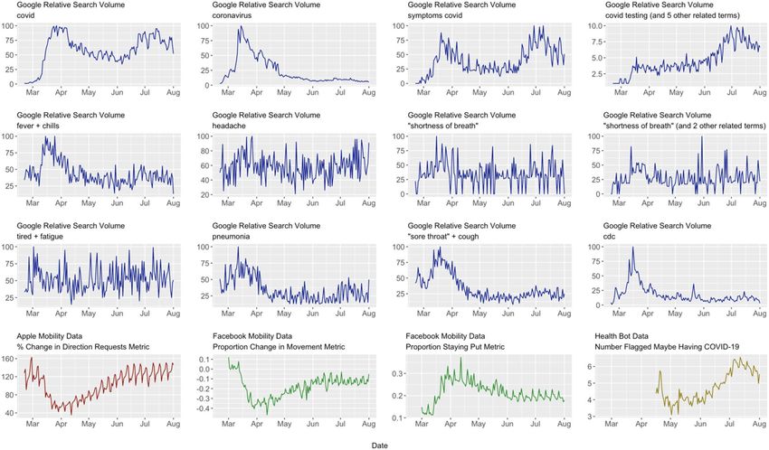
The 16 time plots for the Internet variables are shown in Fig. 1. The first three rows are for those from Google
Trends, while the last row contain those from Apple, Facebook, and Health Bot. Clearly, several of the time series
are visibly nonstationary.
In looking at the maximum absolute Spearman’s correlation coefficient between Census and each Internet
variable across lags 0, − 1, …, − 14, two variables stood out (Table 2). The first was Health Bot, with a maximum
absolute correlation coefficient of 0.865 at time t – 4. The second was the Google Trends search term for covid
testing + covid test + covid19 testing + covid19 test + covid 19 testing + covid 19 test, henceforth, referred to as
Testing. Testing had a maximum absolute correlation coefficient of 0.819 at time t. Three other search terms
were noted, but their maximum absolute correlation coefficients were substantially lower than HealthBot and
Testing. For covid and symptoms covid, it was felt their searches might substantially overlap with Testing. The
search term coronavirus had a negative correlation, likely attributable to people’s initial interest in the novelty
Scientific Reports | (2021) 11:5106 | https://doi.org/10.1038/s41598-021-84091-2 4
Vol:.(1234567890)www.nature.com/scientificreports/
Figure 1. Time plots for internet variables used in data analysis.
Internet variable Lag (in days from time t) Maximum correlation (in absolute magnitude)
covid − 13 0.518
coronavirus 0 − 0.565
symptoms covid − 14 0.614
covid testing (and 5 other related terms) 0 0.819
fever + chills 0 − 0.322
headache −5 0.083
“shortness of breath” 0 − 0.073
“shortness of breath” (and 2 other related terms − 13 0.156
tired + fatigue − 13 0.125
pneumonia −1 − 0.453
“sore throat” + cough 0 − 0.478
cdc 0 − 0.448
Apple mobility 0 0.378
Facebook movement − 14 0.153
Facebook staying put − 14 − 0.109
Health Bot −4 0.865
Table 2. Internet variables and maximum absolute correlation with census in previous 14 days.
of COVID-19, which waned over time, as reflected from the beginning of June onward when RSV values for
coronavirus were quite small. Therefore, for the sake of parsimony, the three other search terms were not con-
sidered further for this research.
After examination of scatter plots, and in preparation for modeling, we transformed both Health Bot (by
taking the natural logarithm) and Testing (by taking the square root) to linearize the relationship between each
of these variables and Census. We then generated longitudinal “cross-correlation”-type of profiles for Health Bot
and Testing using Pearson’s correlation coefficients for lags 0, − 1, …, − 14 as shown in Fig. 2. We can see strong
correlations, all well above 0.80, throughout the time period under consideration.
To better understand the relationships among the three time series, we normalized both the Health Bot and
Census time series to the same [0, 100] scale as Testing, and obtained the results in Fig. 3. Both the Testing and
Health Bot time series appear to share common features of the Census time series (e.g., approximate linear
Scientific Reports | (2021) 11:5106 | https://doi.org/10.1038/s41598-021-84091-2 5
Vol.:(0123456789)www.nature.com/scientificreports/
Figure 2. Longitudinal cross-correlation profiles for census and the two internet variables health bot and
testing.
Figure 3. Multivariate time series plot for census and the two internet variables health bot and testing.
increase from mid-May until mid-July). There is also the suggestion that both the Testing and Health Bot time
series “lead” the Census time. For example, from mid-April until the beginning of May, Health Bot shows a
downward linear trend and this behavior is mirrored in the Census time series roughly one week later.
Using the methodology of Pfaff45 and Dickey and Fuller46, all three time series are nonstationary. Specifi-
cally, the Census time series is difference-stationary, while the Health Bot and Testing time series are both
trend-stationary.
Results from examining AIC values after fitting a VAR model to Census, Testing, and Health Bot, sequentially
increasing the lag order up to 10, were inconclusive. Therefore, we chose the minimum value of K = 2. Johansen’s
procedure (using the trace test version) indicated that two cointegrating vectors should be used. A comparison
of the two AIC values for restricted VECM models described in the Methods suggested placing µ inside the
Scientific Reports | (2021) 11:5106 | https://doi.org/10.1038/s41598-021-84091-2 6
Vol:.(1234567890)www.nature.com/scientificreports/
Parameter Estimate Standard Error
γ1 0.0424 0.0931
γ2 − 3.8514 2.5773
γ3 − 1.3412 0.8382
α1 1.6559* 0.7837
α2 4.3317* 2.1967
Table 3. Results from fitted VECM. Results denoted with an asterisk are statistically significant at a
significance level of 0.05. The estimates for α1 and α2 are normalized.
Parameter Estimate
ρ1 − 1.9911
ρ2 − 2.9994
β1 − 0.0257
β2 − 0.0131
Table 4. Results from fitted VECM. The estimates for all parameters are normalized.
error correction term (AIC = 212.598) as opposed to not doing so (AIC = 217.592). This was also corroborated
by a likelihood ratio test for no linear trend (p-value = 0.32).
For the sake of brevity, and because we are most interested in modeling Census, we only show the portion of
the fitted VECM pertaining to Census. Both α and β are not unique, so it is typical in practice to normalize them.
The normalization we used is the Phillips triangular representation, as suggested by J ohansen51. The expression
for Census in scalar form using general notation is:
�Censust = γ1 �Censust−1 +γ2 �HealthBott−1 +γ3 �Testingt−1 +α1 CR1,t−1 +· · ·+α2 CR2,t−1 +εt
where γ1 , γ2, and γ3 are the corresponding elements of Γ 1, α1 and α2 are the corresponding elements of α, and
CR1 and CR2 are the first and second cointegrated relationships. Collectively, α1 CR1,t−1 and α2 CR2,t−1 are the
error correction terms. In our case, we obtained the results shown in Table 3:
An overall omnibus test for the Census component of the VECM was statistically significant (F0 = 3.393 on
5 and 101 degrees of freedom; p-value = 0.0071). We see that the long-run effects for both cointegrated relation-
ships were important in modeling the first difference of Census at time t. However, the short-run, transitory
effects as measured by first differences of Census, Health Bot, and Testing at lag 1 were not statistically significant.
Furthermore, the expressions for the cointegrated relationships are:
CR1,t−1 = Testingt−1 + β1 Censust−1 + ρ1
CR2,t−1 = HealthBott−1 + β2 Censust−1 + ρ2
where ρ1 and ρ2 are the corresponding elements of ρ , and β1 and β2 are the corresponding elements of β . We
obtained the results shown in Table 4:
Considering the model, parameter estimates from the previous two tables, and looking at CR1,t−1, we see
that if Testing is unusually low relative to Census at time t − 1, so that Testingt−1 < −0.0257Censust−1 − 1.9911,
then this suggests a decrease in Census at time t. Similarly for CR2,t−1, if Health Bot is unusually low relative
to Census at time t − 1, so that HealthBott−1 < −0.0131Censust−1 − 2.9994 , then this suggests a decrease in
Census at time t.
A check of the modulus of all the eigenvalues from the companion matrix associated with the VECM showed
them all to be well below 1, suggesting stability of the model. Inspection of the two fitted cointegration relation-
ships β ′1 y t−1 and β ′2 y t−1 did not suggest any nonstationarity.
Results from the Portmanteau test for serially correlation suggested the presence of serially correlated errors
(p-value = 0.0035). Inspection of all nine acf and ccf plots of the residuals for lags between -15-to-15 identified
the likely reason. The acf plots for Testing and Health Bot showed mild autocorrelation at lag 7. This can be
attributed to a “day of the week” seasonal effect. We address this further in the Discussion. Turning our attention
towards the normality of the errors, the univariate Jarque–Bera test for Health Bot suggested a departure from
this model assumption (p-value = 0.0001). This was attributed to the presence of two mild statistical outliers
early on in the time series. Since these values were otherwise practically unremarkable and with no assignable
cause, we did not remove them.
Figure 4 shows the VECM fit for Census on August 1, 2020. The red line corresponds to the predictions and
forecasts (or “fitted values”) from the model, the black dots are the observations, the blue envelope is the approxi-
mate in-sample 95% prediction interval band, and the pink envelope is, in this case, the 14-days-ahead out-of-
sample forecast interval cone. Up to August 1, the model fit evidences quite reasonable accuracy and precision.
Scientific Reports | (2021) 11:5106 | https://doi.org/10.1038/s41598-021-84091-2 7
Vol.:(0123456789)www.nature.com/scientificreports/
Figure 4. Fitted VECM for census and 14-days-ahead out-of-sample forecast.
Figure 5. Distribution of 7-days-ahead out-of-sample MAPE under time series cross-validation.
We have included the 14 actual Census values that were subsequently observed from August 2-to-August 15.
The corresponding MAPE is 6.4%. While there is clearly a large outlying value on August 4, the VECM forecast
captures the salient feature of the Census counts; that is, a declining local trend. It is interesting to observe the
declining trend in Testing and Health Bot in late July (Fig. 3).
In Fig. 5, we show the distribution of 7-days-ahead out-of-sample MAPE using our time series cross-valida-
tion procedure described in the Methods (n = 88). The distribution is clearly right-skewed. The median MAPE
is 10.5%, while the 95th percentile is 32.9%. In the context of pandemic surveillance and planning, we interpret
these results to suggest our MAPE exhibits very good accuracy of the Census forecast, on average. Ceteris paribus,
a MAPE beyond 32.9% would be unusual and worthy of further investigation.
Scientific Reports | (2021) 11:5106 | https://doi.org/10.1038/s41598-021-84091-2 8
Vol:.(1234567890)www.nature.com/scientificreports/
When we looked at 7-days-ahead out-of-sample MAPE for the ARIMA model using time series cross-vali-
dation, the median MAPE was 8.3%, which was smaller than the value of 10.5% for the VECM. Whether or not
this difference is statistically significant would require additional rigor, which is not done here.
Discussion
In this study, a VECM model inclusive of Internet variables that reflect human behavior during a pandemic
performed very well at 7-day forecasting for a regional health system’s COVID-19 hospital census. In terms of
short-run fluctuations, there is insufficient evidence that lag 1 values of the three differenced series are useful
for prediction of the differenced Census time series. However, in terms of long-run equilibrium, both the error
correction terms are statistically significant. Although all three time series, Census, Testing, and HealthBot, are
nonstationary, their cointegrating relationships allows to predict the change in Census using the VECM.
There are several advantages in adopting our approach. We have conducted a much more thorough search
for candidate Internet variables than what we have observed in the current literature during this pandemic and
employed more rigorous statistical methods. Not only have we used Google Trends search terms, but we also
evaluated mobility data from Facebook and Apple. Further, we have added data from a healthcare chatbot specifi-
cally constructed to assess risk of having COVID-19. Our approach is statistically more rigorous to the extent that
we did not stop at stating correlations, but rather provided a formalized multivariate time series model that can
be potentially used to provide highly accurate forecasts for health system leaders. We know of no other straight-
forward approach in statistics that allows one to simultaneously model nonstationary time series in a multivari-
ate framework and subsequently generate forecasts. Lastly, using time series cross-validation in the manner we
have described here also provides a way of quantifying forecasting performance for various metrics. The VECM
can be easily fit using base R and a few additional packages and we make our code publicly available on GitHub.
The research we have done here can be extended to look at other potential variables that may be leading
indicators for predicting COVID-19 Census. These include the community-level effective reproduction number
Rt 56 and the daily community-level COVID-19 infection incidence, among other examples. Additionally, this
same methodology described herein can be extended to look at other health system relevant outcomes, like ICU
counts, ventilator counts, or hospital daily admissions.
During our specified time period, both the VECM and the ARIMA model provided very good forecasting
performance as measured by MAPE, with the VECM returning a slightly larger MAPE value on average. Other
performance metrics (e.g., RMSE) were not considered here. During the 88 days used for this comparison, the
Health Bot and Testing time series were relatively stable with respect to linear trend. Using the PELT (Pruned
Exact Linear Time) method in the EnvCpt R package, we found two linear trend changepoints for the Health
Bot time series (on 05/28/20 and 07/04/20) and one for the Testing time series (on 06/21/20). How the VECM
would compare to an ARIMA model if the time series under consideration were to exhibit different types of
behaviors would require a further sensitivity study using simulation. We add that just prior to submission (Sep-
tember 26) we refit the VECM and compared it to the ARIMA model. Interestingly, the VECM 7-day forecast
projections were trending upward, while those from the ARIMA model were trending downward. A week later,
when we computed out-of-sample MAPE for the week of September 27th, we obtained 18.1% for the ARIMA
model and 6.8% for the VECM. In fact, Census was beginning to climb. Looking at a multivariate time series
plot similar to Fig. 3, we observed both Testing and Health Bot start to rise in mid-September and then roughly
a week later, Census started to rise.
It is worth mentioning that the VECM is no more or less immune to the same problems we can encounter in
obtaining good forecasts when working with any other models. For example, in order to have good forecasts, the
future must resemble the past. In the midst of a pandemic, other variables can be introduced with the potential
to dramatically alter observed behavior. If a shelter-in-place order, say, were to go in effect in the midst of the
forecast horizons and significantly dampen infection spread, then forecasting performance in that time frame
would likely suffer. In this scenario, no model will work well.
A potential criticism of our work will likely be that the strong correlations we see between Health Bot and
Census, and Testing and Census are “spurious”, being attributable to chance or some underlying unobserved
lurking variable. We feel though it is a reasonable assumption that those individuals in the greater Charlotte
area that are becoming sick with COVID-19 are likely to search Google for a nearby test site (Testing) or take
Atrium Health’s online risk assessment (HealthBot), and then as symptoms subsequently progress proceed to
one of Atrium Health’s facilities to be hospitalized.
This study had several limitations, the first three of which are more specific to the field of i nfodemiology42,57.
First, in terms of data collection, Google’s designation of the Charlotte NC metro area does not perfectly spatially
align with Atrium Health’s core market. Also, Facebook and Apple Map is biased towards users who have enabled
their location history on their mobile devices in order to be detected. Second, the time series in this study were
not collected using any probabilistic sampling design; rather, they were collected using convenience sampling.
Hence, we should be cautious about generalizability of our results. Third, when working with data pulled from
the internet, there is always the chance that the data could be made unavailable or be altered in some way, thus
threatening the durability of such models. We were fortunate in that one of our two important Internet variables
was from Atrium Health’s own public-facing Microsoft Azure HealthBot, at least in part mitigating this risk for
our model. Lastly, perhaps the biggest limitation is that the relationships we have observed in this research could
change at any point in the future so that our model is no longer predictive. Stated another way, because these time
series are nonstationary, they might not stay in sync over long periods of time as their cross-correlations change.
We initially considered other simpler time series regression models (e.g., autoregressive distributed lag
model). However, this approach requires time series under consideration to all be stationary, which ours were
not. A spurious regression will result when one nonstationary time series is regressed against one or more other
Scientific Reports | (2021) 11:5106 | https://doi.org/10.1038/s41598-021-84091-2 9
Vol.:(0123456789)www.nature.com/scientificreports/
nonstationary time series. Hence, we initially spent a considerable effort trying to stationarize our variables (using
differencing, taking logs), and then using lagged versions of the variables before fitting a regression model. In
assessing model fit, we were unsuccessful with this approach. Ultimately, the best way to work with nonstationary
time series in our case was to acknowledge the cointegration of the variables under study.
Because these are variables derived from the internet, it would not be unexpected to see evidence of seasonal
effects in their time series (e.g., day of the week, weekend versus weekday, etc.). For Testing and Health Bot,
we noted the presence of mild autocorrelation in the errors at lag 7. While our VECM results are already very
good, incorporating seasonality into our analysis perhaps might improve forecasting performance. What are
some options to do this? One approach would be to add seasonal effects directly to the VECM (through d t ).
However, with 7 days a week, this would add 18 effect parameters to the model. As we discovered in our case,
if many of these effects were unimportant, then this would negatively affect model fit. It is also important to
understand that this approach makes the assumption that seasonality is deterministic; whereas, we may actually
have stochastic seasonality. A second approach would be to deseasonalize the time series before modeling, i.e.,
a two-stage approach. We deseasonalized the three time series using seasonal decomposition by loess58, noting
that the seasonal effects were relatively small. After repeating our data analysis, we found that the VECM fit was
not as good. A third approach we leave as a future research topic would be to look at initially fitting a VAR(7)
model but disregarding some of the lags (e.g., keeping lags 1 and 7 to address the seasonality, but without the
lags 2–6, say). This would require more intensive programming in R. With any of these approaches, one still has
to check the model for goodness-of-fit and assumptions on the errors; specifically, multivariate normality and
lack of serial correlation.
Our VECM model provides a useful forecasting tool that can guide data-driven decision making as health
system leaders continue to navigate the COVID-19 pandemic. In exploring candidate predictors, valuable insight
was gained as to the relationship between the Internet variables and the hospital census. Both the Health Bot
and the Testing time series from the previous 14 days are strongly informative regarding the hospital COVID-19
census and twice gave ample lead time to a substantial change in the census. The VECM provides another model
for the hospital COVID-19 positive census in case the simpler ARIMA model no longer exhibits a good fit. It
also provides another candidate model that can be used for model-averaged forecasting. While the statistical
underpinning of the VECM is somewhat complex, we found the model outputs to be intuitive and thus easily
communicated to clinical leaders. Access to this information can help better inform manpower planning and
resource allocation throughout the health care system by leveraging insights derived using both of these Internet
variables. For these reasons, it is worth considering adding a VECM to the repertoire of a COVID-19 pandemic
surveillance program.
Received: 2 November 2020; Accepted: 8 February 2021
References
1. World Health Organization. IHR Emergency Committee on Novel Coronavirus (2019-nCoV). https://www.who.int/dg/speeches/
detail/who-director-general-s-statement-on-ihr-emergency-committee-on-novel-coronavirus-(2019-ncov) (2020).
2. COVID-19 Map. Johns Hopkins Coronavirus Resource Center https://coronavirus.jhu.edu/map.html.
3. Centers for Disease Control and Prevention. Coronavirus Disease 2019 (COVID-19). Centers for Disease Control and Prevention
https://www.cdc.gov/coronavirus/2019-ncov/index.html (2020).
4. Jin, Y.-H. et al. A rapid advice guideline for the diagnosis and treatment of 2019 novel coronavirus (2019-nCoV) infected pneu-
monia (standard version). Mil. Med. Res. 7, 4 (2020).
5. Fowler, J. H., Hill, S. J., Obradovich, N. & Levin, R. The effect of stay-at-home orders on COVID-19 cases and fatalities in the United
States. doi:https://doi.org/10.1101/2020.04.13.20063628 (2020).
6. Matrajt, L. & Leung, T. Evaluating the effectiveness of social distancing interventions to delay or flatten the epidemic curve of
coronavirus disease. Emerg. Infect. Dis. 26, (2020).
7. Opening Up America Again. The White House https://www.whitehouse.gov/openingamerica/.
8. Public Health Guidance for Reopening. https://www.alabamapublichealth.gov/covid19/guidance.html.
9. Yamana, T., Pei, S., Kandula, S. & Shaman, J. Projection of COVID-19 Cases and Deaths in the US as Individual States Re-open May
4, 2020.https://doi.org/10.1101/2020.05.04.20090670 (2020).
10. Chopra, V., Toner, E., Waldhorn, R. & Washer, L. How should U.S. hospitals prepare for coronavirus disease 2019 (COVID-19)?
Ann. Intern. Med. 172, 621–622 (2020).
11. Murthy, S., Gomersall, C. D. & Fowler, R. A. Care for critically ill patients with COVID-19. JAMA 323, 1499–1500 (2020).
12. Ng, K. et al. COVID-19 and the risk to health care workers: A case report. Ann. Intern. Med. 172, 766–767 (2020).
13. Mavragani, A. Infodemiology and Infoveillance: Scoping review. J. Med. Internet. Res. 22, e16206 (2020).
14. Althouse, B. M., Ng, Y. Y. & Cummings, D. A. T. Prediction of dengue incidence using search query surveillance. PLoS Negl. Trop.
Dis. 5, e1258 (2011).
15. Husnayain, A., Fuad, A. & Su, E.C.-Y. Applications of Google Search Trends for risk communication in infectious disease manage-
ment: A case study of the COVID-19 outbreak in Taiwan. Int. J. Infect. Dis. 95, 221–223 (2020).
16. Santillana, M., Nsoesie, E. O., Mekaru, S. R., Scales, D. & Brownstein, J. S. Using clinicians’ search query data to monitor influenza
epidemics. Clin. Infect. Dis. Off. Publ. Infect. Dis. Soc. Am. 59, 1446–1450 (2014).
17. Ocampo, A. J., Chunara, R. & Brownstein, J. S. Using search queries for malaria surveillance Thailand. Malar. J. 12, 390 (2013).
18. Google Trends. Google Trends https://trends.google.com/trends/?geo=US.
19. Effenberger, M. et al. Association of the COVID-19 pandemic with internet search volumes: A google TrendsTM analysis. Int. J.
Infect. Dis. 95, 192–197 (2020).
20. Li, C. et al. Retrospective analysis of the possibility of predicting the COVID-19 outbreak from Internet searches and social media
data, China, 2020. Euro Surveill. Bull. Eur. Sur Mal. Transm. Eur. Commun. Dis. Bull. 25, (2020).
21. Walker, A., Hopkins, C. & Surda, P. Use of Google Trends to investigate loss-of-smell-related searches during the COVID-19
outbreak. Int. Forum Allergy Rhinol. 10, 839–847 (2020).
22. Yuan, X. et al. Trends and prediction in daily new cases and deaths of COVID-19 in the United States: An internet search-interest
based model. Explor. Res. Hypothesis Med. 5, 1–6 (2020).
23. Nuti, S. V. et al. The use of google trends in health care research: A systematic review. PLoS ONE 9, e109583 (2014).
Scientific Reports | (2021) 11:5106 | https://doi.org/10.1038/s41598-021-84091-2 10
Vol:.(1234567890)www.nature.com/scientificreports/
24. Cartenì, A., Di Francesco, L. & Martino, M. How mobility habits influenced the spread of the COVID-19 pandemic: Results from
the Italian case study. Sci. Total Environ. 741, 140489 (2020).
25. Jiang, J. & Luo, L. Influence of population mobility on the novel coronavirus disease (COVID-19) epidemic: Based on panel data
from Hubei China. Glob. Health Res. Policy 5, 30 (2020).
26. Kraemer, M. U. G. et al. The effect of human mobility and control measures on the COVID-19 epidemic in China. Science 368,
493–497 (2020).
27. Badr, H. S. et al. Association between mobility patterns and COVID-19 transmission in the USA: A mathematical modelling study.
Lancet Infect. Dis. S1473309920305533 (2020). https://doi.org/10.1016/S1473-3099(20)30553-3.
28. Sasidharan, M., Singh, A., Torbaghan, M. E. & Parlikad, A. K. A vulnerability-based approach to human-mobility reduction for
countering COVID-19 transmission in London while considering local air quality. Sci. Total Environ. 741, 140515 (2020).
29. COVID-19 Community Mobility Report. COVID-19 Community Mobility Report https://www.google.com/covid19/mobility?hl=en.
30. Covid-19 social distancing scoreboard—Unacast. https://www.unacast.com/covid19/social-distancing-scoreboard.
31. University of Maryland COVID-19 impact analysis platform. https://data.covid.umd.edu/.
32. COVID‑19—Mobility Trends Reports. Apple https://www.apple.com/covid19/mobility.
33. Facebook Data for Good Mobility Dashboard. COVID-19 Mobility Data Network https://www.covid19mobility.org/dashboards/
facebook-data-for-good/ (2020).
34. Bharti, U. et al. Medbot: Conversational artificial intelligence powered chatbot for delivering tele-health after COVID-19. in 2020
5th International Conference on Communication and Electronics Systems (ICCES) 870–875 (2020). https://doi.org/10.1109/ICCES
48766.2020.9137944.
35. Ting, D. S. W., Carin, L., Dzau, V. & Wong, T. Y. Digital technology and COVID-19. Nat. Med. 26, 459–461 (2020).
36. Microsoft Health Bot Project - AI At Work For Your Patients. Microsoft Research https://www.microsoft.com/en-us/research/proje
ct/health-bot/.
37. Covid19 Symptom Checker. intermountainhealthcare.org https://i nterm ounta inhea lthca re.o
rg/c ovid1 9-c orona virus/c ovid1 9-s ympt
om-checker/.
38. WHO Health Alert brings COVID-19 facts to billions via WhatsApp. https://web.archive.org/web/20200323042822/https://www.
who.int/news-room/feature-stories/detail/who-health-alert-brings-covid-19-facts-to-billions-via-whatsapp (2020).
39. Miner, A. S., Laranjo, L. & Kocaballi, A. B. Chatbots in the fight against the COVID-19 pandemic. Npj Digit. Med. 3, 1–4 (2020).
40. Stankiewicz, C. F., Kevin. Apple updated Siri to help people who ask if they have the coronavirus. CNBC https://www.cnbc.com/
2020/03/21/apple-updated-siri-to-help-people-who-ask-if-they-have-coronavirus.html (2020).
41. Explore—Opendatasoft. https://demography.osbm.nc.gov/explore/?sort=modifi ed.
42. Eysenbach, G. Infodemiology and infoveillance: Tracking online health information and cyberbehavior for public health. Am. J.
Prev. Med. 40, S154–S158 (2011).
43. Mavragani, A. & Ochoa, G. Google trends in infodemiology and infoveillance: Methodology framework. JMIR Public Health
Surveill 5, e13439 (2019).
44. Google News Initiative Training Center. Google News Initiative Training Center https://newsinitiative.withgoogle.com/training/
lesson/6043276230524928?image=trends&tool=Google%20Trends.
45. Pfaff, B. Analysis of integrated and cointegrated time series with R. (Springer-Verlag, 2008). https:// d oi. org/ 1 0. 1 007/
978-0-387-75967-8.
46. Dickey, D. A. & Fuller, W. A. Likelihood ratio statistics for autoregressive time series with a unit root. Econometrica 49, 1057–1072
(1981).
47. Campbell, J. Y. & Perron, P. Pitfalls and opportunities: What macroeconomists should know about unit roots. NBER Macroecon.
Annu. 6, 141–201 (1991).
48. Akaike, H. A new look at the statistical model identification. IEEE Trans. Autom. Control 19, 716–723 (1974).
49. Burnham, K. P. & Anderson, D. R. Model selection and multimodel inference: a practical information-theoretic approach. (Springer,
2002).
50. Johansen, S. Estimation and hypothesis testing of cointegration vectors in Gaussian vector autoregressive models. Econometrica
59, 1551–1580 (1991).
51. Johansen, S. Likelihood-Based Inference in Cointegrated Vector Autoregressive Models Oxford University Press. N. Y. (1995).
52. Johansen, S. & Juselius, K. Maximum likelihood estimation and inference on cointegration—with appucations to the demand for
money. Oxf. Bull. Econ. Stat. 52, 169–210 (1990).
53. Hamilton, J. Time series analysis (Princeton, Princeton University Press, 1994).
54. Zivot, E. & Wang, J. Modeling financial time series with S-Plus®. (Springer New York, 2003). https://d oi.org/1 0.1 007/
978-0-387-21763-5.
55. Hyndman, R. J. & Khandakar, Y. Automatic time series forecasting: the forecast package for R. J. Stat. Softw. 27, (2008).
56. Cori, A., Ferguson, N. M., Fraser, C. & Cauchemez, S. A new framework and software to estimate time-varying reproduction
numbers during epidemics. Am. J. Epidemiol. 178, 1505–1512 (2013).
57. Barros, J. M., Duggan, J. & Rebholz-Schuhmann, D. The application of internet-based sources for public health surveillance
(infoveillance): Systematic review. J. Med. Internet. Res. 22, e13680 (2020).
58. Cleveland, R. B., Cleveland, W. S., McRae, J. E. & Terpenning, I. STL: A seasonal-trend decomposition procedure based on loess.
J. Off. Stat. 6, 3–73 (1990).
Author contributions
PT conceived of and conducted the statistical analysis, and wrote much of the manuscript text; TT helped with
the statistical analysis and wrote portions of the manuscript text; GR and AW performed critical revision of
the manuscript for important intellectual content and offered guidance in the study. All authors reviewed the
manuscript.
Competing interests
The authors declare no competing interests.
Additional information
Correspondence and requests for materials should be addressed to P.J.T.
Reprints and permissions information is available at www.nature.com/reprints.
Publisher’s note Springer Nature remains neutral with regard to jurisdictional claims in published maps and
institutional affiliations.
Scientific Reports | (2021) 11:5106 | https://doi.org/10.1038/s41598-021-84091-2 11
Vol.:(0123456789)www.nature.com/scientificreports/
Open Access This article is licensed under a Creative Commons Attribution 4.0 International
License, which permits use, sharing, adaptation, distribution and reproduction in any medium or
format, as long as you give appropriate credit to the original author(s) and the source, provide a link to the
Creative Commons licence, and indicate if changes were made. The images or other third party material in this
article are included in the article’s Creative Commons licence, unless indicated otherwise in a credit line to the
material. If material is not included in the article’s Creative Commons licence and your intended use is not
permitted by statutory regulation or exceeds the permitted use, you will need to obtain permission directly from
the copyright holder. To view a copy of this licence, visit http://creativecommons.org/licenses/by/4.0/.
© The Author(s) 2021, corrected publication 2021
Scientific Reports | (2021) 11:5106 | https://doi.org/10.1038/s41598-021-84091-2 12
Vol:.(1234567890)You can also read