A clustering-based approach to ocean model-data comparison around Antarctica - Ocean Science
←
→
Page content transcription
If your browser does not render page correctly, please read the page content below
Ocean Sci., 17, 131–145, 2021
https://doi.org/10.5194/os-17-131-2021
© Author(s) 2021. This work is distributed under
the Creative Commons Attribution 4.0 License.

A clustering-based approach to ocean model–data comparison
around Antarctica
Qiang Sun1 , Christopher M. Little1 , Alice M. Barthel2 , and Laurie Padman3
1 Atmospheric  and Environmental Research, Inc., Lexington, MA 02421, USA
2 Los Alamos National Laboratory, Los Alamos, NM 87545, USA
3 Earth and Space Research, 3350 SW Cascade Ave., Corvallis, OR 97333, USA

Correspondence: Qiang Sun (qsun@aer.com)

Received: 19 May 2020 – Discussion started: 4 June 2020
Revised: 9 November 2020 – Accepted: 23 November 2020 – Published: 19 January 2021

Abstract. The Antarctic Continental Shelf seas (ACSS) are a         highlights that the relative differences between regimes and
critical, rapidly changing element of the Earth system. Anal-       the locations where each regime dominates are well repre-
yses of global-scale general circulation model (GCM) simu-          sented in the model. CESM2 is generally fresher and warmer
lations, including those available through the Coupled Model        than WOA and has a limited fresh-water-enriched coastal
Intercomparison Project, Phase 6 (CMIP6), can help reveal           regimes. Given the sparsity of observations of the ACSS, this
the origins of observed changes and predict the future evo-         technique is a promising tool for the evaluation of a larger
lution of the ACSS. However, an evaluation of ACSS hy-              model ensemble (e.g., CMIP6) on a circum-Antarctic basis.
drography in GCMs is vital: previous CMIP ensembles ex-
hibit substantial mean-state biases (reflecting, for example,
misplaced water masses) with a wide inter-model spread.
                                                                    1   Introduction
Because the ACSS are also a sparely sampled region, grid-
point-based model assessments are of limited value. Our goal        The Antarctic Continental Shelf seas (ACSS, defined here
is to demonstrate the utility of clustering tools for identifying   as the ocean regions adjacent to Antarctica with water depth
hydrographic regimes that are common to different source            shallower than 2500 m) are critical components of the cli-
fields (model or data), while allowing for biases in other met-     mate system, playing an essential role in ice sheet mass bal-
rics (e.g., water mass core properties) and shifts in region        ance, sea ice formation and ocean circulation (Rignot et al.,
boundaries. We apply K-means clustering to hydrographic             2008; Hobbs et al., 2016; Bindoff et al., 2000). ACSS ocean
metrics based on the stratification from one GCM (Com-              state and the climate system components that are coupled to it
munity Earth System Model version 2; CESM2) and one                 are changing rapidly. In the Amundsen–Bellingshausen seas
observation-based product (World Ocean Atlas 2018; WOA),            sectors, the atmosphere (Bromwich et al., 2013) and subsur-
focusing on the Amundsen, Bellingshausen and Ross seas.             face ocean (Schmidtko et al., 2014) are warming, the sea-ice-
When applied to WOA temperature and salinity profiles,              free period is rapidly increasing (Stammerjohn et al., 2012),
clustering identifies “primary” and “mixed” regimes that            ice shelves are thinning (Rignot et al., 2013; Paolo et al.,
have physically interpretable bases. For example, meltwater-        2015; Adusumilli et al., 2020) and the grounded portion of
freshened coastal currents in the Amundsen Sea and a re-            the ice sheet is losing mass at an accelerating rate (Shepherd
gion of high-salinity shelf water formation in the southwest-       et al., 2018; Sutterley et al., 2014; Gardner et al., 2018). The
ern Ross Sea emerge naturally from the algorithm. Both re-          Ross Sea has also experienced long-term changes in freshwa-
gions also exhibit clearly differentiated inner- and outer-shelf    ter content (Jacobs and Giulivi, 2010; Castagno et al., 2019)
regimes. The same analysis applied to CESM2 demonstrates            and an increase in sea ice production and extent (Parkinson,
that, although mean-state model biases in water mass T –S           2019; Holland et al., 2017).
characteristics can be substantial, using a clustering approach

Published by Copernicus Publications on behalf of the European Geosciences Union.
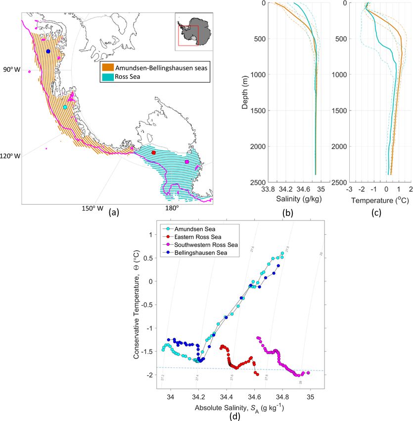
132                       Q. Sun et al.: A clustering-based approach to ocean model–data comparison around Antarctica

   Assessing the causes of observed changes in climate and         properties in the Amundsen–Bellingshausen seas are simi-
the coastal cryosphere and their future evolution requires         lar, with cold and fresh water overlying relatively warm and
coupled, global atmosphere–ocean general circulation mod-          salty water. In the Ross Sea, water properties are different on
els (GCMs). However, recent GCMs exhibit large biases rel-         its southwestern and eastern sides, mainly distinguished by
ative to modern observations and a wide inter-model spread         their salinity (Fig. 1d).
(Agosta et al., 2015; Sallée et al., 2013; Rickard and Behrens,       The sparseness of measurements in the ACSS also aggra-
2016; Hosking et al., 2016; Little and Urban, 2016; Barthel        vates errors associated with gridded observational products.
et al., 2020). These modern-state biases suggest the potential     Coastal regions, in particular, are subject to substantial er-
for large uncertainties in the projected ocean state, including    rors. Sun et al. (2019) showed that salinity biases between
the vertical and horizontal distribution of ocean heat, with       WOA objective analysis and the World Ocean Database in-
significant consequences for the accuracy of projections of        crease toward coastlines. The gridded objective analysis field
the effect of the ACSS on other climate components (e.g.,          neglects the dynamical processes governing water mass mod-
Sallée et al., 2013; Agosta et al., 2015). For example, De-        ifications and circulations induced by complex continen-
Conto and Pollard (2016) projected extreme rates of 21st-          tal shelf bathymetry (Dunn and Ridgway, 2002; Schmidtko
century ice sheet mass loss from the Pacific sector for a high-    et al., 2013). In sparsely sampled regions, grid-point-based
emission scenario. However, their projections were forced          comparisons (e.g., Little and Urban, 2016) are thus of lim-
using a single GCM (CCSM4) that required a +3 ◦ C correc-          ited utility and may underestimate uncertainty in the refer-
tion to subsurface water temperatures in the Amundsen Sea          ence (observational) product. We suggest that it is often more
to match observed hydrography and modern ice shelf melt            meaningful to assess GCMs using a regionally averaged ap-
rates. This significant bias correction indicates an underly-      proach.
ing mean-state error (e.g., a misplaced water mass) that casts        Previous model–data comparisons in the ACSS have em-
substantial doubt on the projected future ocean state in that      ployed strategies such as averaging over a priori defined
specific model.                                                    regions (e.g., Barthel et al., 2020). Such methods are ill-
   The first step toward identifying the physical processes un-    equipped to assess model biases resulting from misplaced
derlying GCM representation errors is assessing the magni-         water masses. An alternative method is objective cluster-
tude and spatial distribution of biases. However, such a strat-    ing, which can be used to identify regions of similar hydro-
egy must account for strong horizontal and vertical gradients      graphic metrics. For example, Hjelmervik and Hjelmervik
in ACSS hydrographic properties (see, e.g., Orsi and Wieder-       (2013) demonstrated the application of a clustering-based ap-
wohl, 2009; Thompson et al., 2018) and the sparseness and          proach using Argo profiles to segregate the North Atlantic
variable quality of available observations (e.g., Schmidtko        into groups with similar vertical T and S profiles separated
et al., 2014). Strong gradients are evident in the Amundsen,       by fronts.
Bellingshausen and Ross seas (ABRS) sector of the ACSS.               The results of clustering analyses are dependent on the
There, the time-mean ocean state of the objectively analyzed       metrics chosen for the analysis. For example, metrics could
temperature and salinity field, as represented in the 0.25◦        be chosen as the layer thicknesses of water masses defined
World Ocean Atlas version 2018 (WOA hereafter), suggests           by T , S and neutral density. Schmidtko et al. (2014) parti-
that the ABRS can be roughly separated into two geographi-         tioned water masses in the Southern Ocean into Winter Wa-
cal regions, the Amundsen–Bellingshausen seas and the Ross         ter (WW), CDW, and Antarctic Shelf Bottom Water (ASBW)
Sea (Fig. 1a). In the Ross Sea, dense water formation occurs       using only temperature. However, their metrics of subsurface
locally, through brine rejection from winter sea ice formation     water temperature maxima and minima are ineffective on the
in coastal polynyas, resulting in regionally averaged water        continental shelf, where temperature profiles are often com-
well below 0 ◦ C at water depths of 100 to 700 m (Fig. 1c). At     plex and show strong lateral variability in water properties
the same depth range in the Amundsen–Bellingshausen seas,          (Fig. 1d). Sallée et al. (2013) proposed a method to use po-
water temperatures can reach +1.2 ◦ C due to the presence of       tential vorticity evaluated from density profiles and the lo-
Circumpolar Deep Water (CDW).                                      cal salinity minimum at 30◦ S to distinguish vertical water
   In addition to these stark contrasts in regional mean tem-      masses in the Southern Ocean.
perature (and salinity), there is also significant spatial vari-      In the ACSS, however, the hydrographic structure is com-
ability within each region of the ABRS and across the conti-       plicated not only by the variability of primary water masses
nental shelf break. For example, Fig. 1 indicates a high stan-     but also by transport, mixing, and strong and highly local-
dard deviation (SD) in ocean temperature on the continental        ized interactions between the atmosphere, ocean, sea ice, and
shelf with water depth shallower than 700 m (0.5 ◦ C in the        ice shelves. Each of these processes is sensitive to vertical
Amundsen–Bellingshausen seas and 1.4 ◦ C in the Ross Sea).         and horizontal density gradients and gradients in bathymetry.
Much of this variability is attributable to the lateral temper-    Metrics that capture the importance of stratification concur-
ature gradient from the subsurface layer of CDW over the           rently with dominant water mass characteristics provide the
continental slope to the modified (cooled) water masses in-        best test of whether a model is representing the principal
shore. In the alongshore direction, vertical profiles of water     dynamical processes governing hydrographic variability in

Ocean Sci., 17, 131–145, 2021                                                          https://doi.org/10.5194/os-17-131-2021
Q. Sun et al.: A clustering-based approach to ocean model–data comparison around Antarctica                                            133

Figure 1. (a) The study domain of Amundsen–Bellingshausen seas and Ross Sea with bathymetry above 2500 m. The magenta line indicates
the 1000 m IBCSO depth contour. Panels (b) and (c) show geographically averaged decadal (1995–2004) WOA salinity and temperature pro-
files in the Amundsen–Bellingshausen seas (orange; corresponding to the orange stippled region in a) and the Ross Sea (cyan; corresponding
to the cyan stippled region in a). Dashed lines indicate ±1 SD of values at each depth in each region. (d) T –S properties of selected water
columns (corresponding to colored circles in a).

the ACSS. Here, we develop new metrics targeted at ACSS                 processing procedures of the WOA are detailed in Locarnini
hydrography and assess the utility of a clustering-based ap-            et al. (2019) for temperature and Zweng et al. (2019) for
proach for model–data comparison.                                       salinity. This study focuses on the domain from the west of
                                                                        Cape Adare (163◦ E) on the western side of the Ross Sea to
                                                                        the southern end of Alexander Island (76◦ W), at depths be-
2     Methods                                                           tween 0 and 2500 m. The landward limit of the study domain
                                                                        is the Antarctic coast and the ice shelf edges as identified in
In this paper, we identify hydrographic regimes and their T –           Fig. 1a.
S properties using metrics derived from three-dimensional                  We compare the Community Earth System Model ver-
grids of measured and modeled temperature and salinity                  sion 2 (CESM2; Danabasoglu et al., 2020) to WOA for the
(Sect. 2.1) using a K-means clustering method (Sect. 2.2).              same period and domain. The time-mean model salinity and
We then apply a clustering algorithm based on data density              temperature fields over the 1995–2004 period are calculated
to exclude outliers (Sect. 2.3) from the resulting “groups”.            from the monthly output of the Coupled Model Intercom-
                                                                        parison Project Phase 6 (CMIP6) historical simulation (ex-
2.1    Data and processing                                              periment tag r1i1p1f1) (Eyring et al., 2016) at the native
                                                                        ocean model resolution (roughly 1◦ in longitude and 0.5◦
We use decadal-mean, objectively analyzed T and S fields
                                                                        in latitude). CESM2 uses the CICE5 (Hunke et al., 2015)
from WOA for 1995–2004, with 0.25◦ resolution in both lat-
                                                                        sea ice model; however, dynamic and thermodynamic in-
itude and longitude. The data sources, quality controls and

https://doi.org/10.5194/os-17-131-2021                                                                   Ocean Sci., 17, 131–145, 2021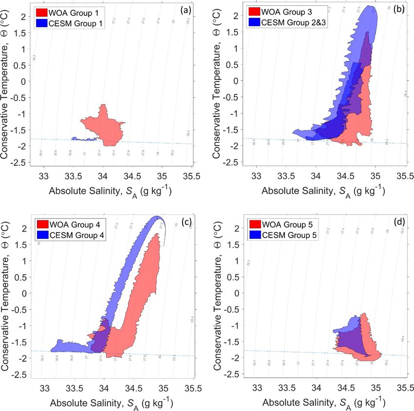
134                                Q. Sun et al.: A clustering-based approach to ocean model–data comparison around Antarctica

teractions with land ice are not represented (Danabasoglu              Table 1. The radius ε used in the DBSCAN for WOA and CESM2.
et al., 2020). The CMIP6 forcing data are described in Eyring
et al. (2016) and can be download from input4MIPs (https:                          Group 1     Group 2   Group 3   Group 4   Group 5
//esgf-node.llnl.gov/search/input4MIPs, last access: 15 Oc-              WOA           0.05       0.05      0.04      0.03      0.03
tober 2020).                                                             CESM2        0.045       0.04      0.06     0.035      0.04
   We used the Gibbs SeaWater (GSW) Oceanographic Tool-
box of TEOS–10 (McDougall and Barker, 2011) to calcu-                  Table 2. The coverage (%) of the majority group of DBSCAN in
late seawater properties. The absolute salinity (SA ) is given         the total non-outlier data.
in units of g kg−1 , and conservative temperature (2) is given
in ◦ C. All seawater temperatures are referenced to the sea                        Group 1     Group 2   Group 3   Group 4   Group 5
surface.                                                                 WOA           99.6       97.9      99.9      100        100
                                                                         CESM2          100       97.3      99.5      99.9      99.7
2.2   Prototype-based clustering technique (K-means)

The K-means clustering analysis used in this study is an un-
supervised learning technique that classifies data into mean-          with different clustering evaluation methods (e.g., the elbow
ingful groups based on their similarity. In this study, the simi-      method; Thorndike, 1953) and different domains. The selec-
larity is defined by two metrics of the water column: (1) salin-       tion of K is thus based not only on the results of silhouette
ity at the temperature minimum and (2) salinity at the temper-         assessment but also on the ability to interpret the groups as
ature maximum. The rationale for these choices is discussed            representative of different underlying physical processes (see
in Sect. 3.1.                                                          Sect. 3).
   The K-means algorithm is initialized by randomly select-
ing data in N dimensions (here, N = 2, for the two speci-              2.3   Density-based clustering technique
fied metrics) for a specified number of groups (K). For each
                                                                       In subsequent sections, we use a T –S diagram to compare
group (ki ), the sum of squared distance (SSD) of each data
                                                                       the properties of groups given by the K-means algorithm.
point (ξ ) to the group’s centroid (ci ) is calculated as follows:
                                                                       We applied a data-density-based clustering technique (DB-
           K X                                                         SCAN) (Ester et al., 1996) to define the “core” of a group
           X                                        1 X
SSD =                  dist(ci , ξ )2   with ci =           ξ,   (1)   and to exclude outliers on the T –S diagram. Note that DB-
           i=1 ξ ∈ki
                                                    mi ξ ∈k            SCAN is only used to highlight the core of a given group and
                                                          i
                                                                       facilitate comparisons of water properties between WOA and
where dist is the standard distance between data and centroid          CESM2.
in N -dimensional Euclidean data space and mi is the total                The T –S core of each hydrographic regime identified by
number of data points in group ki . The algorithm iterates to          the K-means clustering is determined by the DBSCAN al-
minimize SSD by adjusting the centroids, recalculating the             gorithm using two parameters: a radius (ε) and a minimum
distances and redistributing data points among the groups.             number of neighboring points (MinPts). The DBSCAN al-
The K-means algorithm will have multiple solutions because             gorithm builds up pools of data by initially choosing a ran-
it is initialized with randomly selected data. We apply the K-         dom data point. If the initially chosen data point has less
means 1000 times and choose the solution with the lowest               than MinPts within ε, then it is defined as an outlier. If
SSD for analysis.                                                      this data point has more than MinPts within ε, then a pool
    The K-means algorithm requires specification of the num-           of data is initialized consisting of the initial point and the
ber of groups (K). We use silhouette scores si (n) (Eq. 2) to          points within ε (neighbors). The pool grows by continually
assess the appropriate values of K.                                    clustering neighboring points until these points have fewer
            b(ξ ) − a(ξ )                                              than MinPts within ε. The algorithm continues until all data
si (n) =                                                         (2)   points are either clustered into pools of data or labeled as
           max{a(ξ ), b(ξ )}
                                                                       outliers.
                                                                            √ In the current study, we choose MinPts = 10 and
    In Eq. (2), n represents the number of data points in group        ε = S 2 + T 2 . The value of ε is then selected (Table 1) so
ki , a(ξ ) is the mean dist from a data point ξ to all other data      that the largest pool of data contains at least 97 % of non-
points within the group ki and b(ξ ) is mean dist from ξ to            outlier points (Table 2). This pool of data constitutes the core
all other data points outside the group ki . Silhouette scores         of each group.
are evaluated for each data point ξ in the group ki and range
between −1 and 1. If ξ lies perfectly at the centroid of group
ki , then si (n) = 1.
    A rigid interpretation of the silhouette algorithm would
choose the value of K that corresponds to the highest mean
value of si (n). However, the optimal K value can vary

Ocean Sci., 17, 131–145, 2021                                                                 https://doi.org/10.5194/os-17-131-2021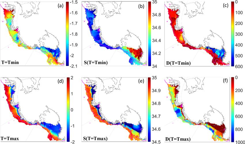
Q. Sun et al.: A clustering-based approach to ocean model–data comparison around Antarctica 135
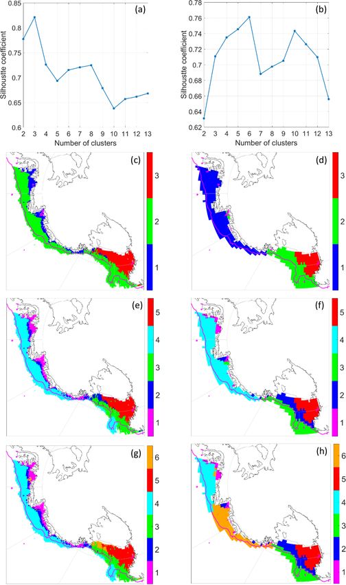
3 Results spatial distributions of groups 3, 5 and 6 in the ABRS are
shown in Fig. 3c–h.
3.1 Defining water column metrics When WOA data are clustered into three groups (Fig. 3c),
the K-means algorithm segregates the water close to the
Our goal in this analysis is to utilize key features of local Antarctic coast from the water on the shelf and continen-
water columns to identify regions with similar hydrographic tal slope. The coastal domains are further distinguished into
properties. Such metrics must be able to capture stratifica- Amundsen–Bellingshausen coastal waters and Ross coastal
tion, and the changes in T and S in both along- and cross- waters. By increasing the number of groups to five (Fig. 3e),
shelf directions. For the ACSS, the metrics must include a narrow domain between coastal and shelf waters emerges.
salinity because it is the dominant factor influencing water In the Ross Sea, waters on the shelf and across the shelf break
column stability and reflects critical processes such as brine are segregated into two groups. For K = 6 (Fig. 3g), the
input during sea ice formation, and freshwater inputs from southeastern coastal domain of the Ross Sea (orange) is fur-
melting sea ice and ice shelves. By itself, however, salinity ther separated from the narrow domain between coastal and
poorly represents the vertical composition of water masses shelf waters in the Amundsen–Bellingshausen seas, while the
since it increases monotonically with water depth over most locations of the other groups are generally unchanged.
of the ACSS (Fig. 1); salinity alone is insufficient to identify Examining the groups with respect to the two metrics used
regimes with sub-surface heat reservoirs that are character- in the K-means clustering (Fig. 4) shows that, when K = 3,
istic of regions with high ice shelf basal melt rates (Rignot the groups are separated by the perpendicular lines from the
et al., 2013; Dinniman et al., 2016; Adusumilli et al., 2020). incenter of the triangular T –S distributions (Fig. 4a). As the
The metrics we use in this study – salinity at the vertical total number of groups increases, data points are progres-
temperature minimum and salinity at the vertical tempera- sively divided into smaller subsets, with an asymmetry that
ture maximum – are similar to those used by Timmermans is influenced by their original distribution in our two-metric
et al. (2014) to segregate surface water from Alaskan coastal parameter space, as well as gaps and discontinuities (Fig. 4c
water in the Central Canada Basin of the Arctic Ocean. and e).
Along-shelf variations of water properties are evident in In CESM2, the clusters in the ABRS differ from those
salinity at the vertical temperature minimum (Fig. 2b). In the for WOA, particularly for K = 3 and K = 6. For K = 3
Amundsen–Bellingshausen seas, the depth of minimum tem- (Fig. 3d), the entire Amundsen–Bellingshausen seas region
perature (Fig. 2c) is commonly above 200 m, where salin- is segregated from the Ross Sea, while the southwestern
ity is often less than 34.2 g kg−1 . In contrast, in the south- Ross Sea is still recognized as an independent group. For
western Ross Sea, the minimum temperature is usually lo- K = 6, the Amundsen Sea is segregated from the Belling-
cated below 350 m and coincides with much higher salin- shausen Sea. With K = 5 (Fig. 3f), CESM2 clustering is
ity (> 34.8 g kg−1 ). The northwestern Ross Sea contains qualitatively similar to WOA, with a coastal group emerges
a regime with a local temperature minimum at shallower in the Amundsen–Bellingshausen seas; however, its areal ex-
depths approaching the shelf break, but its salinity (between tent is much smaller than in WOA. In the Ross Sea, the water
34.2 to 34.6 g kg−1 ) is higher than near-surface water in the on the continental shelf is separated from the water on the
Amundsen–Bellingshausen seas. continental slope, similar to WOA. CESM2 shows a similar
The salinity at the vertical temperature maximum shows range to WOA in metric space (Fig. 4), although with much
pronounced variations in the cross-shelf direction (Fig. 2d– larger gaps. In particular, CESM2 has substantially fewer
f). The maximum water temperature (Fig. 2d) is commonly data points with intermediate and low salinity (Fig. 4b). In-
found at depths above 200 m close to the coast and ice creasing K for clustering analysis of CESM2 output subdi-
shelves (Fig. 2f) and deeper toward the shelf break and over vides high-salinity regimes at Tmax based on the distribution
the continental slope where the water depth increases. The of salinity at Tmin (Fig. 4d and f).
salinity at the vertical maximal temperature (Fig. 2e) shows Based on the silhouette scores, the optimum clustering
similar variations in the cross-shelf direction, with lower for CESM2 is six groups; however, the WOA data have a
salinity (< 34.7 g kg−1 ) near the coast and ice shelves and maximum silhouette score for K = 3. Segregating the WOA
higher salinity (> 34.8 g kg−1 ) on the continental shelves and into five or six groups is reasonable, as the clustering al-
near the shelf break. gorithm continually distinguishes finer differences in the
coastal regimes (Fig. 3e and g). However, the segregation of
3.2 Evaluating the optimum number of groups CESM2 into six groups (Fig. 3h) is physically unfair since
the water properties below the surface layers are nearly in-
We used the mean value of the silhouette score si (n) in distinguishable between the Amundsen and Bellingshausen
Eq. (2) to evaluate an appropriate number of groups (K) for seas (Fig. 1d). Figure 4 also indicates that the segregation of
WOA and CESM2, testing 2 ≤ K ≤ 13 (Fig. 3). For WOA, Amundsen–Bellingshausen seas regions in CESM2 is a re-
the highest value of si occurs when K = 3; for CESM2, sult of discontinuities between groups 1 and 5 (Fig. 4f). We
K = 6 has the highest silhouette score (Fig. 3a and b). The thus choose to use five groups for the rest of the study. Our
https://doi.org/10.5194/os-17-131-2021 Ocean Sci., 17, 131–145, 2021
136                               Q. Sun et al.: A clustering-based approach to ocean model–data comparison around Antarctica

Figure 2. Clustering metrics in WOA. Minimum temperature at each grid point (a) and the salinity (b) and water depth at the minimum
temperature. Panels (d)–(f) are the same as (a)–(c) but for quantities at the temperature maximum.

Table 3. The salinity and temperature standard deviation of WOA               by weak vertical gradients in both T and S over the ∼ 400 m
(at depth of 500 m if not specified).                                         water column (Fig. 5a). The water in this group has relatively
                                                                              low salinity (33.8 to 34.5 g kg−1 ), temperature close to the
                           Salinity (g kg−1 )           Temperature (◦ C)     freezing point (generally lower than −1 ◦ C) and low density
                        Amundsen and       Ross       Amundsen and     Ross   (26.9 and 27.5 kg m−3 ) (Fig. 6a), which suggests that the wa-
                        Bellingshausen                Bellingshausen          ter in this regime is strongly influenced by coastal freshwater
  Geography             0.16 (200 m)       0.11       0.84 (200 m)     1.37   input (Moffat et al., 2008; Jacobs and Giulivi, 2010; Jourdain
                                 0.10                          1.42           et al., 2017).
                                                                                 Group 2, which is spatially located between the coastal
  K-means         1     0.10 (200 m)            n/a   0.22 (200 m)      n/a
  groups          2              0.07                          1.34           waters (groups 1 and 5) and outer continental shelf waters
                  3     n/a                0.08       n/a              0.97   (groups 3 and 4), represents a narrow domain of mixing
                  4              0.08                          0.44           (Fig. 3e). This regime is characterized by relatively high stan-
                  5     n/a                0.10       n/a              0.17   dard deviations in salinity and temperature at depths between
n/a – not applicable.
                                                                              100 and 700 m, indicating that the location and shape of the
                                                                              thermocline and halocline above the typical depth of the shelf
                                                                              break vary within this group (Fig. 5b). Below 700 m, the
findings from analyzing the temperature and salinity proper-                  range of salinity and temperature are relatively small, due
ties in the following sections further support this decision.                 to reduced the limited amount of data at these depths over
                                                                              the relatively narrow continental slope. In the upper ocean,
3.3     Physical interpretation of WOA groups                                 group 2 has a salinity from 33.8 to 34.7 g kg−1 , temperature
                                                                              from −2 to −0.5 ◦ C and density from 27.1 to 27.8 kg m−3
Vertical profiles of temperature and salinity are shown for                   (Figs. 5b and 6b), lying between the properties of surface
each WOA group in Fig. 5. The mean vertical structure of                      waters in groups 1 and 5. In the subsurface, group 2 has a
each group is clearly different; furthermore, the standard de-                temperature above −0.5 ◦ C and salinity above 34.5 g kg−1 ,
viations at each depth within groups are much smaller than                    which represents modified CDW on the shelf (Carmack,
those of regional mean profiles (Table 3). With these verti-                  1977; Orsi and Wiederwohl, 2009; Emery, 2011).
cal structures as context, we examine T –S properties at all                     Group 3, which is found on the outer continental shelf and
depths from each WOA group in Fig. 6. The DBSCAN al-                          the continental slope of the Ross Sea (Fig. 3e), shows high
gorithm is used to identify the “core” of non-outlier data in                 standard deviations in temperature above 700 m (Fig. 5c),
each group, shown with dark shading in Fig. 6.                                similar to group 2. However, the water in this regime is gen-
   Group 1, which occupies the inshore regions of the                         erally denser than group 2. The surface water in group 3 is
Amundsen–Bellingshausen seas (Fig. 3e), is characterized                      fresher than that of group 5 (Figs. 5c and 6c, f), which may

Ocean Sci., 17, 131–145, 2021                                                                     https://doi.org/10.5194/os-17-131-2021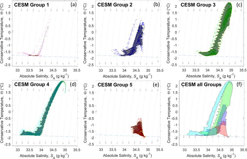
Q. Sun et al.: A clustering-based approach to ocean model–data comparison around Antarctica                                       137

                                                                   Table 4. The percentage of clustered water in the total ocean volume
                                                                   in the ABRS.

                                                                                Group 1    Group 2     Group 3   Group 4   Group 5
                                                                     WOA             1.0        3.6       21.0      62.1       12.3
                                                                     CESM2           0.3        7.2       33.2      50.4        8.9

                                                                   et al. (2014). It has a well-defined vertical temperature struc-
                                                                   ture with limited spatial variability (Fig. 5d). In this region,
                                                                   Winter Water (WW) with salinity of 33.8 to 34.5 g kg−1 , tem-
                                                                   perature of −2 to −0.5 ◦ C and density of 27 to 27.5 g m−3
                                                                   overlies CDW (salinity 34.6 to 36.8 g kg−1 , temperature 0 to
                                                                   +2 ◦ C and density 27.8 to 27.9 g m−3 ), with a mean profile
                                                                   showing a clear transition between them (Fig. 6d).
                                                                      Group 5, in the southwestern Ross Sea with some exten-
                                                                   sions to the southeast (Fig. 3e), has higher salinity than other
                                                                   groups (Fig. 6). The almost uniform vertical temperature pro-
                                                                   file (Fig. 5e) is identified as HSSW. It is characterized by
                                                                   salinity 34.3 to 35.1 g kg−1 , temperature close to the freez-
                                                                   ing point, and density of 27.5 to 28.1 kg m−3 (Fig. 6e), re-
                                                                   sulting from brine rejection in the polynyas along the coast
                                                                   and Ross Ice Shelf front (Foster and Carmack, 1976). The
                                                                   surface portion of the waters in group 5 with salinity lower
                                                                   than 34.62 g kg−1 is often defined as Low-Salinity Shelf Wa-
                                                                   ter (LSSW) in the Ross Sea shelf, but we generally refer to
                                                                   group 5 as HSSW because its volume is much higher than
                                                                   the LSSW (Orsi and Wiederwohl, 2009).
                                                                      Overall, groups 1 and 5 (Fig. 6a and e) show relatively
                                                                   homogeneous salinity and temperature, while group 4 has
                                                                   a pronounced thermocline and halocline at shallow depth.
                                                                   These three groups (1, 4 and 5) represent the three “primary”
                                                                   ABRS hydrographic regimes. In contrast to these primary
                                                                   regimes, groups 2 and 3 have more complex vertical struc-
Figure 3. K-means clustering evaluation for WOA and CESM.          tures, more spatial variability in thermocline at depths above
Silhouette analysis is shown in (a) and (b) for WOA and CESM,      about 600 m (roughly the shelf break) and can be considered
respectively. The geographic regions corresponding to 3, 5 and 6   “mixed” regimes.
groups for WOA, (shown in c, e and g) and for CESM (shown in d,
f and h) are shown.                                                3.4   Assessing groups in CESM2

                                                                   To identify hydrographic regimes in CESM2, we conduct the
result from sea ice melt and/or lateral mixing with fresher        same analyses as described for WOA in the previous section,
shelf water originating in the Amundsen–Bellingshausen             focusing on results for K = 5 (Fig. 3f). The T –S properties
seas (Assmann et al., 2005; Porter et al., 2019). The sub-         of each group in CESM2 are shown in Fig. 7. CESM2 re-
surface water (between 100 and 600 m) of group 3 (Figs. 5c         sults are similar to WOA’s in that three primary regimes are
and 6c) does not have a clear vertical water mass transition,      present (group 1, coastal fresh-water-enriched; group 4, off-
and denser water exhibits a wide temperature range (−1.5           shelf; and group 5, HSSW), but they show differences in their
to +1.5 ◦ C) with relatively high salinity (34.6 to 35 g kg−1 ),   spatial extent (Fig. 3e vs. f), volume (Table 4) and T –S prop-
suggestive of mixing between High-Salinity Shelf Water             erties (Fig. 8).
(HSSW) and CDW.                                                       As in WOA, HSSW (group 5) of CESM2 is localized in
   Group 4, on the continental shelf of the Amundsen–              the southwestern Ross Sea, but its eastward extension into
Bellingshausen seas and along most of the continental slope        the southeastern Ross Sea is missing in CESM2 (Fig. 3e
of the ABRS (Fig. 3e), exhibits properties consistent with         and f), resulting in a reduced HSSW volume (Table 4). The
off-shelf Southern Ocean water, as noted by Schmidtko              coastal fresh-water-enriched regime (group 1) is mostly ab-

https://doi.org/10.5194/os-17-131-2021                                                                Ocean Sci., 17, 131–145, 2021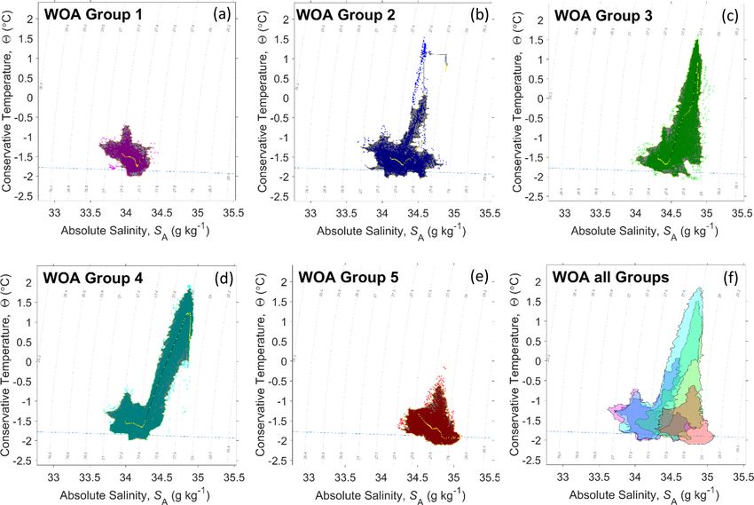
138                       Q. Sun et al.: A clustering-based approach to ocean model–data comparison around Antarctica

Figure 4. ABRS groups in metric space. Each point corresponds to a grid point, with a color corresponding to its group number, for K = 3,
5 and 6, for WOA (shown in a, c and e) and for CESM2 (shown in b, d and f).

sent in CESM2 and is replaced by the off-shelf regime in the           shelf regime) exhibits a fresh bias in WW in the upper water
Amundsen Sea.                                                          column, but the densest off-shelf water in group 4, i.e., CDW,
   Mismatches between CESM2 and WOA are also evident                   is saltier and warmer (Fig. 8c). Sea ice concentrations are bi-
in the T –S properties of these primary regimes. In general,           ased low in CESM due to positive zonal wind stress biases
HSSW in CESM2 has a fresh and warm bias relative to                    in the Southern Ocean (Singh et al., 2020). This wind stress
WOA (Fig. 8d). Combined with its reduced volume relative               bias may, in turn, lead to an overestimate of the upwelling of
to WOA, this bias in CESM2 HSSW properties suggests that               warm and salty CDW onto the ACSS. The limited extent of
weak modeled katabatic winds in the southwestern Ross Sea              the coastal fresh-water-enriched regime (group 1) in CESM2
may limit sea ice production and export. Group 4 (the off-             may result from the absence of basal melt from ice shelves.

Ocean Sci., 17, 131–145, 2021                                                               https://doi.org/10.5194/os-17-131-2021
Q. Sun et al.: A clustering-based approach to ocean model–data comparison around Antarctica                                           139

Figure 5. Mean (solid lines) WOA salinity (in blue) and temperature (in red) profiles for five groups (from a to e) shown in Fig. 3e; ±1 SD
at each depth is shown with dashed lines.

   The mixed regimes shift geographic location in CESM2.                In this parameterization, locations of the on-shore source wa-
The narrow mixing zone (group 2) between coastal fresh-                 ter at its formation regions and off-shore entrainment, which
water-enriched and off-shelf regimes in the Amundsen–                   mixes with the source water to produce the final water mass,
Bellingshausen seas is not evident in CESM2 (Fig. 3e and                are defined, and overflow water is routed to fixed locations.
f); the CESM2 is likely too coarse to resolve these mixing              While this parameterization allows transport of HSSW to the
fronts. In the Ross Sea, groups are separated into on-shelf             Southern Ocean, it is entirely artificial and does not represent
(group 2) and off-shelf (group 3) approximately along the               on-shelf mixing processes.
1000 m isobath (Fig. 3f). CESM2 fails to show the path of
export of Ross on-shelf water (group 2, Fig. 3f) along the              3.5   Assessing clustering over the ACSS
northwestern continental slope (Orsi et al., 1999) as it is seen
in the WOA (group 3, Fig. 3e). The core of on-shelf wa-                 As the K-means algorithm is based on purely statistical crite-
ter (group 2) also has less overlap with HSSW (group 5)                 ria (centroid and minimized SSD in Eq. 1) applied to specific
in the T –S diagram in CESM2 (Fig. 7f) compared to WOA                  metrics, it is valuable to assess whether clustering results are
(Fig. 6f). It is possible that these differences result from the        sensitive to different study domains. As a test case, we ap-
overflow parameterization in CESM2 (Briegleb et al., 2010).             ply the same algorithm to WOA over the entire circumpolar
                                                                        ACSS where total water depth is less than 2500 m. The met-

https://doi.org/10.5194/os-17-131-2021                                                                  Ocean Sci., 17, 131–145, 2021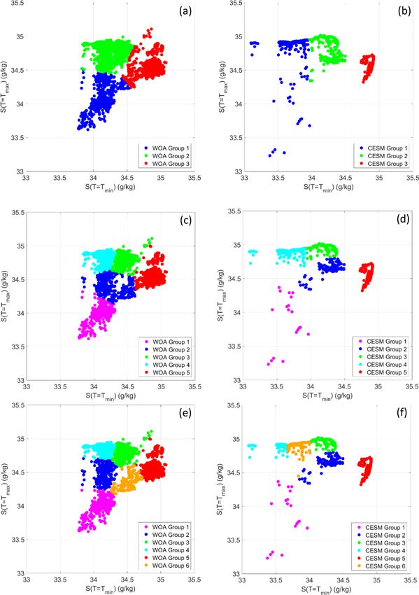
140                        Q. Sun et al.: A clustering-based approach to ocean model–data comparison around Antarctica

Figure 6. T –S properties for the five WOA groups (from a to e) shown in Fig. 3e. The dotted yellow lines show the profile of mean
temperature and salinity in each group, and the dark shaded areas are the cores of water property from the density-based clustering results.
The cores of all five groups are overlaid on the same plot in (f).

Figure 7. As in Fig. 6 but for the five groups identified in CESM2 (from a to e) shown in Fig. 3f.

rics used as input for the K-means analysis, as well as the to-             The location of five clustered water groups over the en-
tal number of groups (K = 5), are unchanged. The use of the              tire ACSS is shown in Fig. 9a. Within the ABRS domain,
uniformly gridded WOA product, rather than observational                 the geographic locations of all groups are almost unchanged,
data, avoids the possibility that the comparison is biased by            indicating the clustering results in the ABRS are insensitive
regional variations in data density.                                     to substantial enlargement of the domain. The region identi-

Ocean Sci., 17, 131–145, 2021                                                                  https://doi.org/10.5194/os-17-131-2021
Q. Sun et al.: A clustering-based approach to ocean model–data comparison around Antarctica 141
fied as group 5 in the southwestern Ross Sea, which is asso-
ciated with HSSW formation, remains. Outside the ABRS,
the clustering approach identifies water of similar properties
to group 5 in the Weddell Sea near the Filchner–Ronne Ice
Shelf, the George V Coast near the Mertz Glacier tongue,
and Bransfield Strait and south of Trinity Peninsula (regions
marked on Fig. 9b). The southern Weddell Sea experiences
similar conditions to the southwestern Ross Sea, with HSSW
formation in winter due to brine rejection from sea ice for-
mation enhanced by katabatic winds and tides driving a nar-
row but persistent along-ice-front polynya (Nicholls et al.,
2009). Along the George V Coast, HSSW is also generated
by similar processes acting near the Mertz Glacier ice tongue
(Bindoff et al., 2000; Post et al., 2011).
The waters in the subsurface of Bransfield Strait and south
of the Trinity Peninsula are also grouped with the HSSW
regions, although their surface water is warmer and fresher
than that of other HSSW regions around Antarctica. Cook
et al. (2016) showed that the regional water properties around
the tip of the Antarctica Peninsula, based on the World Ocean
Database, are very similar to HSSW. Gordon et al. (2000)
Figure 8. The core of water properties in WOA (red) and CESM2 also noted that the water properties in the center of Bransfield
(blue). Note that groups 2 and 3 have been combined for CESM2. Strait are similar to HSSW in the Weddell Sea; they inferred
that these waters are formed in western Weddell Sea coastal
polynyas and flow into Bransfield Strait.
4 Discussion
We have shown that the ABRS can be clustered into differ-
ent regions based on salinity at the vertical water temperature
minimum and maximum. This technique can help identify
regions in model and observational datasets in which wa-
ter properties are controlled by similar physical processes.
This is in contrast to traditional grid-point-based compar-
isons, which do not adequately account for misplaced water
masses.
In this study, WOA has been employed to assess CESM2
results. However, the hydrographic regimes identified in
WOA may be misleading if they result from interpolation
and extrapolation artifacts associated with non-uniform sam-
pling of data in time and space or if the water column struc-
tures are not adequately represented in WOA. One source
of uncertainty in WOA arises from differences between true
and gridded bathymetry, complicating interpolation and ex-
Figure 9. (a) WOA-based groups on the entire ACSS (same color trapolation of sparely sampled data into deeper portions of
code as Fig. 3e). (b) Four places are identified as HSSW regimes the water column. In Fig. 10, we compare the depths of
with the following color coding: blue is the southwestern Ross Sea, the deepest available data in WOA and CESM2 with water
red is the Weddell Sea near the Filchner–Ronne Ice Shelf and the depths in the International Bathymetric Chart of the Southern
George V Coast, cyan is the Bransfield Strait and south of Trinity Ocean (IBCSO, Arndt, et al., 2013). WOA has a clear mis-
Peninsula, and green is the Mertz Glacier tongue. (c) T –S proper- representation of the Amundsen–Bellingshausen seas con-
ties of group 5 (HSSW) regions, with their geographic location and
tinental shelf bathymetry (Fig. 10b). First, the 1000 m iso-
color code matched in (b).
bath is shifted substantially landward in the Amundsen Sea.
Second, deep across-shelf troughs (e.g., in Fig. 10a) are not
represented in the inner shelf of WOA, which possibly af-
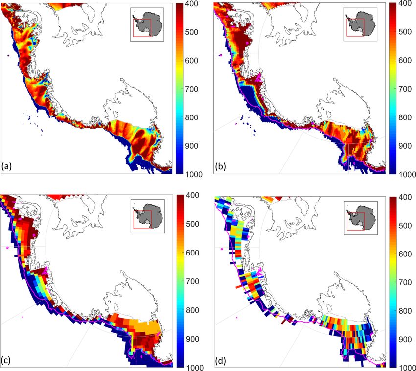
https://doi.org/10.5194/os-17-131-2021 Ocean Sci., 17, 131–145, 2021142 Q. Sun et al.: A clustering-based approach to ocean model–data comparison around Antarctica
is possible to circumvent interpolation-related issues associ-
ated with using scattered and/or sparse data. Such datasets
might include individual observations or model output on
a native grid. For example, the deepest observational tem-
perature measurements in the World Ocean Database 2018
(WOD), even at a 1◦ resolution, show that observations are
available in coastal Amundsen–Bellingshausen seas troughs
that are not present in IBCSO (compare Fig. 10d with a); see
also Padman et al. (2010). More broadly, the WOD-based
salinity and temperature climatology of Sun et al. (2019) re-
veals that its use can avoid biases created by spatial interpo-
lation of shelf water with off-shelf water.
The success of this technique at identifying locations and
properties of HSSW regimes at other locations on the Antarc-
tic continental shelf suggests that it might be used to evaluate
other global and/or regional models on a circum-Antarctic
basis. Other metrics might be employed depending on spe-
cific research goals. For example, the pycnocline depth or
the mean or maximum temperature below a fixed depth may
Figure 10. Bathymetry between 400 and 1000 m of (a) IBCSO be better metrics of subsurface water masses. It will also be
(500 m horizontal resolution), (b) WOA (0.25◦ horizontal resolu- interesting to track water masses and their pathways with
tion), (c) CESM2 (1 × 0.5◦ long/lat resolution) and (d) the WOD metrics based on their characteristic properties. However, we
bin-averaged into 1◦ horizontal resolution with all types of instru- note that comparisons of the locations of groups could be-
ment with temperature measurements. The magenta line indicates
come complex if the approach is applied to multiple models
the 1000 m IBCSO depth contour.
with substantial biases between their representations of spe-
cific water masses.
fects the value of salinity at the temperature maximum be-
cause the CDW is missing in these regions of the Amundsen– 5 Conclusions
Bellingshausen seas.
It is, therefore, unclear whether groups 1 and 2 are sep- We have demonstrated the utility and sensitivity of
arated from the shelf and continental slope waters of group a clustering-based approach for assessing hydrographic
4 in WOA (Fig. 3e) due to their upper-ocean freshwater en- regimes and their water properties on the Antarctic conti-
richment relative to other groups or if the groups are influ- nental shelf, using the World Ocean Atlas objective anal-
enced by under-sampling of hydrography in deep troughs ysis product (WOA) and numerical model output from
of the Amundsen–Bellingshausen seas. We note that the the Community Earth System Model version2 (CESM2).
bathymetry of CESM2 has similar issues to WOA in the We segregated the waters in the ABRS into five physi-
Amundsen–Bellingshausen seas (Fig. 10c). Neither WOA cally interpretable groups using the salinity at the mini-
nor CESM2 represents the water in deep troughs below about mum and maximum temperature of each water column in
300 m in these regions, and thus the differences in the groups the domain. The method identifies High-Salinity Shelf Wa-
between WOA and CESM2, i.e., the missing group 1 in the ter (HSSW), coastal fresh-water-enriched, and off-shelf hy-
Amundsen coast and narrow group 2 in the Bellingshausen drographic regimes in observations and the model. Water
Sea, are unlikely to be due to the bathymetric misrepresenta- on the continental shelf and upper continental slope in the
tion (Fig. 3e and f). We suggest, instead, that the mismatch ABRS generally shows a warm bias in CESM2 compared to
of water properties is likely to be induced by the misrepre- WOA. The near-surface ocean in CESM2 is generally fresher
sentation of freshwater input or unresolved coastal currents than in WOA but lacks a well-defined fresh-water-enriched
in CESM2 (Tseng et al., 2016; Sun et al., 2017). coastal current. In the subsurface, CESM2 is saltier in re-
We have highlighted a key advantage to assessing mod- gions of Circumpolar Deep Water but fresher than WOA
els with clustering-based approaches compared to traditional in HSSW formation regions. Our comparison suggests that
grid-point-based methods: the ability to identify geographic mean-state biases of CESM2 in the ACSS result from both
displacements of hydrographic regimes and to distinguish local and remote processes, including overestimated zonal
these displacements from biases in water mass T –S prop- winds in the Southern Ocean, unrepresented thermodynamic
erties. In addition, this approach minimizes potential biases interactions with ice shelves, and the inadequate representa-
introduced during gridding or re-gridding of data and mod- tion of overflows in the Ross Sea. A more specific investi-
els to a common grid for comparison studies. For example, it gation of coastal processes, Southern Ocean dynamics and
Ocean Sci., 17, 131–145, 2021 https://doi.org/10.5194/os-17-131-2021Q. Sun et al.: A clustering-based approach to ocean model–data comparison around Antarctica 143
atmospheric forcing will help further identify the cause of Agosta, C., Fettweis, X., and Datta, R.: Evaluation of the CMIP5
these biases. models in the aim of regional modelling of the Antarc-
The clustered hydrographic regimes in the ABRS are tic surface mass balance, The Cryosphere, 9, 2311–2321,
largely unchanged when our method is applied to the en- https://doi.org/10.5194/tc-9-2311-2015, 2015.
tire circum-Antarctic Continental Shelf sea area. HSSW- Arndt, J. E., Schenke, H. W., Jakobsson, M., Nitsche, F. O.,
Buys, G., Goleby, B., Rebesco, M., Bohoyo, F., Hong, J.,
characterized regimes emerge in WOA in the southern Wed-
Black, J., Greku, R., Udintsev, G., Barrios, F., Reynoso-
dell Sea, near Mertz Glacier tongue and in Bransfield Strait. Peralta, W., Taisei, M., and Wigley, R.: The International Bathy-
Future work will focus on applying this approach to a wider metric Chart of the Southern Ocean (IBCSO) Version 1.0 – A
range of models (e.g., CMIP6 output and circum-Antarctic new bathymetric compilation covering circum-Antarctic waters,
simulations) and establishing techniques to work with scat- Geophys. Res. Lett., 40, 3111–3117, 2013.
tered observational data. Finally, we note that the cluster- Assmann, K. M., Hellmer, H. H., and Jacobs, S. S.: Amundsen
ing results for the ACSS based on the WOA decadal data Sea ice production and transport, J. Geophys. Res.-Oceans, 110,
(1995–2004) are consistent with the results based on the most C12013, https://doi.org/10.1029/2004JC002797, 2005.
modern WOA decadal data (2005–2017). However, cluster- Barthel, A., Agosta, C., Little, C. M., Hattermann, T., Jourdain,
ing, applied to a variety of metrics, provides the potential to N. C., Goelzer, H., Nowicki, S., Seroussi, H., Straneo, F., and
identify more subtle temporal changes in hydrographic fields Bracegirdle, T. J.: CMIP5 model selection for ISMIP6 ice sheet
model forcing: Greenland and Antarctica, The Cryosphere, 14,
such as changes in regime extent in the absence of significant
855–879, https://doi.org/10.5194/tc-14-855-2020, 2020.
changes in water mass characteristics in the ACSS. Bindoff, N. L., Rosenberg, M. A., and Warner, M. J.: On the circu-
lation and water masses over the Antarctic continental slope and
rise between 80 and 150 E, Deep-Sea Res. Pt. II, 47, 2299–2326,
Data availability. The data used in this study are publicly avail- 2000.
able via the links below: World Ocean Atlas 2018 at https:// Briegleb, B. P., Danabasoglu, G., and Large, W. G.: An
www.nodc.noaa.gov/OC5/woa18/woa18data.html (NOAA, 2021a); Overflow parameterization for the ocean component of the
World Ocean Database 2018 at https://www.nodc.noaa.gov/OC5/ Community Climate System Model, University Corpora-
WOD/pr_wod.html (NOAA, 2021b); and CESM2 data at https: tion for Atmospheric Research, No. NCAR/TN-481+STR,
//esgf-node.llnl.gov/search/cmip6/ (WCRP, 2021). https://doi.org/10.5065/D69K4863, 2010.
Bromwich, D. H., Nicolas, J. P., Monaghan, A. J., Lazzara, M. A.,
Keller, L. M., Weidner, G. A., and Wilson, A. B.: Central West
Author contributions. QS performed the analyses and wrote the ar- Antarctica among the most rapidly warming regions on Earth,
ticle. CML, AMB, and LP conceived the research idea, directed the Nat. Geosci., 6, 139–145, https://doi.org/10.1038/ngeo1671,
project, and supported the article revision. 2013.
Carmack, E. C.: Water characteristics of the Southern Ocean south
of the Polar Front, in: Voyage of Discovery: George Deacon 70th
Competing interests. The authors declare that they have no conflict Anniversary, edited by: Angel, M., Pergamon, Oxford, 1977.
of interest. Castagno, P., Capozzi, V., DiTullio, G. R., Falco, P., Fusco, G., Rin-
toul, S. R., Spezie, G., and Budillon, G.: Rebound of shelf water
salinity in the Ross Sea, Nat. Commun., 10, 1–6, 2019.
Acknowledgements. The authors thank the NCAR climate model- Cook, A. J., Holland, P. R., Meredith, M. P., Murray, T., Luck-
ing groups for producing and distributing the CESM2 output. man, A., and Vaughan, D. G.: Ocean forcing of glacier retreat in
the western Antarctic Peninsula, Science, 353, 283–286, 2016.
Danabasoglu, G., Lamarque, J. F., Bachmeister, J., Bailey, D. A.,
DuVivier, A. K., Edwards, J., Emmons, L. K., Fasullo, J.,
Financial support. This research has been supported by the NSF
Garcia, R., Gettelman, A., Hannay, C., Holland, M. M.,
(grant no. 1744789), NASA (grant no. NNX17AG63G), and the
Large, W. G., Lawrence, D. M., Lenaerts, J. T. M., Lind-
DOE (HiLAT-RASM project).
say, K., Lipscomb, W. H., Mills, M. J., Neale, R., Ole-
son, K. W., Otto-Bliesner, B., Phillips, A. S., Sacks, W.,
Tilmes, S., van Kampenhout, L., Vertenstein, M., Bertini, A.,
Review statement. This paper was edited by Trevor McDougall and Dennis, J., Deser, C., Fischer, C., Fox-Kember, B., Kay, J. E.,
reviewed by two anonymous referees. Kinnison, D., Kushner, P. J., Long, M. C., Mickelson, S.,
Moore, J. K., Nienhouse, E., Polvani, L., Rasch, P. J., and
Strand, W. G.: The Community Earth System Model version
2 (CESM2), J. Adv. Model. Earth Sy., 12, e2019MS001916,
References https://doi.org/10.1029/2019MS001916, 2020.
DeConto, R. M. and Pollard, D.: Contribution of Antarctica to past
Adusumilli, S., Fricker, H. A., Medley, B., Padman, L., and and future sea-level rise, Nature, 531, 591–597, 2016.
Siegfried, M. R.: Interannual variations in meltwater input to Dinniman, M. S., Asay-Davis, X. S., Galton-Fenzi, B. K., Hol-
the Southern Ocean from Antarctic ice shelves, Nat. Geosci., 13, land, P. R., Jenkins, A., and Timmermann, R.: Modeling ice
616–620, 2020.
https://doi.org/10.5194/os-17-131-2021 Ocean Sci., 17, 131–145, 2021144 Q. Sun et al.: A clustering-based approach to ocean model–data comparison around Antarctica
shelf/ocean interaction in Antarctica: A review, Oceanography, Locarnini, R. A., Mishonov, A. V., Baranova, O. K., Boyer, T. P.,
29, 144–153, 2016. Zweng, M. M., Garcia, H. E., Reagan, J. R., Seidov, D., Weath-
Dunn, J. R. and Ridgway, K. R.: Mapping ocean properties in re- ers, K. W., Paver, C. R., and Smolyar, I. V.: World Ocean At-
gions of complex topography, Deep-Sea Res. Pt. I, 49, 591–604, las 2018, Volume 1: Temperature, in: NOAA Atlas NESDIS 81,
2002. edited by: Mishonov, A., available at: https://archimer.ifremer.fr/
Emery, W. J.: Water types and water masses, Encyclopedia of Ocean doc/00651/76338/ (last access: 16 January 2021), 2019.
Sciences, 6, 3179–3187, 2011. McDougall, T. J. and Barker, P. M.: Getting started with TEOS-
Ester, M., Kriegel, H. P., Sander, J., and Xu, X.: A density-based 10 and the Gibbs Seawater (GSW) oceanographic toolbox,
algorithm for discovering clusters in large spatial databases with SCOR/IAPSO WG, 127, 1–28, ISBN: 978-0-6465-5621-5, 2011.
noise, KDD, 96, 226–231, 1996. Moffat, C., Beardsley, R. C., Owens, B., and Van Lipzig, N.: A first
Eyring, V., Bony, S., Meehl, G. A., Senior, C. A., Stevens, B., description of the Antarctic Peninsula Coastal Current, Deep-Sea
Stouffer, R. J., and Taylor, K. E.: Overview of the Coupled Res. Pt. II, 55, 277–293, 2008.
Model Intercomparison Project Phase 6 (CMIP6) experimen- Nicholls, K. W., Østerhus, S., Makinson, K., Gammelsrød, T., and
tal design and organization, Geosci. Model Dev., 9, 1937–1958, Fahrbach, E.: Ice-ocean processes over the continental shelf of
https://doi.org/10.5194/gmd-9-1937-2016, 2016. the southern Weddell Sea Antarctica: A review, Rev. Geophys.,
Foster, T. D. and Carmack, E. C.: Frontal zone mixing and Antarctic 47, RG3003, https://doi.org/10.1029/2007RG000250, 2009.
Bottom Water formation in the southern Weddell Sea, Deep Sea NOAA: World Ocean Atlas 2018, available at: https://www.
Research and Oceanographic Abstracts, 23, 301–317, 1976. nodc.noaa.gov/OC5/woa18/woa18data.html, last access: 16 Jan-
Gardner, A. S., Moholdt, G., Scambos, T., Fahnstock, M., uary 2021a.
Ligtenberg, S., van den Broeke, M., and Nilsson, J.: In- NOAA: World Ocean Database 2018, available at: https://www.
creased West Antarctic and unchanged East Antarctic ice dis- nodc.noaa.gov/OC5/WOD/pr_wod.html, last access: 16 Jan-
charge over the last 7 years, The Cryosphere, 12, 521–547, uary 2021b.
https://doi.org/10.5194/tc-12-521-2018, 2018. Orsi, A. H. and Wiederwohl, C. L.: A recount of Ross Sea waters,
Gordon, A. L., Mensch, M., Zhaoqian, D., Smethie Jr., W. M., and Deep-Sea Res. Pt. II, 56, 778–795, 2009.
De Bettencourt, J.: Deep and bottom water of the Bransfield Orsi, A. H., Johnson, G. C., and Bullister, J. L.: Circulation, mixing,
Strait eastern and central basins, J. Geophys. Res.-Oceans, 105, and production of Antarctic Bottom Water, Prog. Oceanogr., 43,
11337–11346, 2000. 55–109, 1999.
Hjelmervik, K. T. and Hjelmervik, K.: Improved estimation of Padman, L., Costa, D. P., Bolmer, S. T., Goebel, M. E.,
oceanographic climatology using empirical orthogonal func- Huckstadt, L. A., Jenkins, A., McDonald, B. I., and
tions and clustering, in: 2013 MTS/IEEE OCEANS-Bergen, Shoosmith, D. R.: Seals map bathymetry of the Antarc-
1–5, IEEE, Bergen, Norway, https://doi.org/10.1109/OCEANS- tic continental shelf, Geophys. Res. Lett., 37, L21601,
Bergen.2013.6607987, 2013. https://doi.org/10.1029/2010GL044921, 2010.
Hobbs, W. R., Massom, R., Stammerjohn, S., Reid, P., Williams, G., Paolo, F. S., Fricker, H. A., and Padman, L.: Volume loss from
and Meier, W.: A review of recent changes in Southern Ocean sea Antarctic ice shelves is accelerating, Science, 348, 327–331,
ice, their drivers and forcings, Global Planet. Change, 143, 228– 2015.
250, 2016. Parkinsona, C. L.: A 40-y record reveals gradual Antarctic sea ice
Holland, M. M., Landrum, L., Raphael, M., and Stammerjohn, S.: increases followed by decreases at rates far exceeding the rates
Springtime winds drive Ross Sea ice variability and change in seen in the Arctic, P. Natl. Acad. Sci. USA, 116, 14414–14423,
the following autumn, Nat. Commun., 8, 1–8, 2017. 2019.
Hosking, J. S., Orr, A., Bracegirdle, T. J., and Turner, J.: Future cir- Porter, F. D., Springer, S. R., Padman, Laurie, Fricker, Helen A.,
culation changes off West Antarctica: Sensitivity of the Amund- Tinto, K. J., Riser, S. C., Bell, R. E., the ROSETTA-Ice Team:
sen Sea Low to projected anthropogenic forcing, Geophys. Res. volution of the Seasonal Surface Mixed Layerof the Ross Sea,
Lett., 43, 367–376, 2016. Antarctica, ObservedWith Autonomous Profiling Floats, J. Geo-
Hunke, E. C., Lipscomb, W. H., Turner, A. K., Jeffery, N., and El- phys. Res.-Oceans, 124, 4934–4953, 2019.
liott, S.: CICE: The Los Alamos Sea Ice Model, Documentation Post, A. L., Beaman, R. J., O’Brien, P. E., Eléaume, M., and Rid-
and Software User’s Manual, Version 5.1, T-3 Fluid Dynamics dle, M. J.: Community structure and benthic habitats across the
Group, Los Alamos National Laboratory, Tech. Rep. LA-CC-06- George V Shelf, East Antarctica: trends through space and time,
012, 2015. Deep-Sea Res. Pt. II, 58, 105–118, 2011.
Jacobs, S. S. and Giulivi, C. F.: Large multidecadal salinity trends Rickard, G. and Behrens, E.: CMIP5 Earth system models with bio-
near the Pacific–Antarctic continental margin, J. Climate, 23, geochemistry: A Ross Sea assessment, Antarct. Sci., 28, 327–
4508–4524, 2010. 346, 2016.
Jourdain, N. C., Mathiot, P., Merino, N., Durand, G., Le Sommer, J., Rignot, E., Bamber, J. L., Van Den Broeke, M. R., Davis, C., Li, Y.,
Spence, P., Dutrieux, P., and Madec, G.: Ocean circulation and Van De Berg, W. J., and Van Meijgaard, E.: Recent Antarctic ice
sea-ice thinning induced by melting ice shelves in the Amundsen mass loss from radar interferometry and regional climate mod-
Sea, J. Geophys. Res.-Oceans, 122, 2550–2573, 2017. elling, Nat. Geosci., 1, 106–110, 2008.
Little, C. M. and Urban, N. M.: CMIP5 temperature biases and 21st Rignot, E., Jacobs, S., Mouginot, E., and Scheuchl, B.: Ice-shelf
century warming around the Antarctic coast, Ann. Glaciol., 57, melting around Antarctica, Science, 341, 266–270, 2013.
69–78, 2016. Sallée, J. B., Shuckburgh, E., Bruneau, N., Meijers, A. J., Bracegir-
dle, T. J., Wang, Z., and Roy, T.: Assessment of Southern Ocean
Ocean Sci., 17, 131–145, 2021 https://doi.org/10.5194/os-17-131-2021Q. Sun et al.: A clustering-based approach to ocean model–data comparison around Antarctica 145 water mass circulation and characteristics in CMIP5 models: Sun, Q., Whitney, M. M., Bryan, F. O., and Tseng, Y.-h.: A box Historical bias and forcing response, J. Geophys. Res.-Oceans, model for representing estuarine physical processes in Earth sys- 118, 1830–1844, 2013. tem models, Ocean Model., 112, 139–153, 2017. Schmidtko, S., Johnson, G. C., and Lyman, J. M.: MIMOC: A Sun, Q., Whitney, M. M., Bryan, F. O., and Tseng, Y.-h.: As- global monthly isopycnal upper-ocean climatology, J. Geophys. sessing the skill of the improved treatment of riverine freshwa- Res.-Oceans, 118, 1658–1672, 2013. ter in the Community Earth System Model relative to a new Schmidtko, S., Heywood, K. J., Thompson, A. F., and Aoki, S.: salinity climatology, J. Adv. Model. Earth Sy., 11, 1189–1206, Multidecadal warming of Antarctic waters, Science, 346, 1227– https://doi.org/10.1029/2018MS001349, 2019. 1231, 2014. Sutterley, T. C., Velicogna, I., Rignot, E., Mouginot, J., Flament, T., Shepherd, A., Ivins, E., Rignot, E., Smith, B., van den Broeke, M., Van Den Broeke, J. M., Van Wessem, J. M., and Reijmer, C. H.: Velicogna, Is., Whitehouse, P., Briggs, K., Joughin, I., Krin- Mass loss of the Amundsen Sea Embayment of West Antarc- ner, G., Nowicki, S., Payne, T., Scambos, T., Schlegel, N., tica from four independent techniques, Geophys. Res. Lett., 41, Geruo, A., Agosta, C., Ahlstrøm, A., Babonis, G., Barletta, V., 8421–8428, 2014. Blazquez, A., Bonin, J., Csatho, B., Cullather, R., Felikson, D., Thompson, A. F., Stewart, A. L., Spence, P., and Heywood, K. J.: Fettweis, X., Forsberg, R., Gallee, H., Gardner, A., Gilbert, L., The Antarctic Slope Current in a changing climate, Rev. Geo- Groh, A., Gunter, B., Hanna, E., Harig, C., Helm, V., Horvath, A., phys., 56, 741–770, 2018. Horwath, M., Khan, S., Kjeldsen, K. K., Konrad, H., Lan- Thorndike, R. L.: Who Belongs in the Family? Psychometrika, 18, gen, P., Lecavalier, B., Loomis, B., Luthcke, S., McMillan, M., 267–276, 1953. Melini, D., Mernild, S., Mohajerani, Y., Moore, P., Moug- Timmermans, M. L., Proshutinsky, A., Golubeva, E., Jackson, J. M., inot, J., Moyano, G., Muir, A., Nagler, T., Nield, G., Nilsson, J., Krishfield, R., McCall, M., Platov, G., Toole, J., Williams, W., Noel, B., Otosaka, I., Pattle, M. E., Peltier, W. R., Pie, N., Riet- Kikuchi, T., and Nishino, S.: Mechanisms of Pacific summer wa- broek, R., Rott, H., Sandberg-Sørensen, L., Sasgen, I., Save, H., ter variability in the Arctic’s Central Canada Basin, J. Geophys. Scheuchl, B., Schrama, E., Schröder, L., Seo, K.-W., Simon- Res.-Oceans, 119, 7523–7548, 2014. sen, S., Slater, T., Spada, G., Sutterley, T., Talpe, M., Tarasov, L., Tseng, Y.-H., Bryan, F. O., and Whitney, M. M.: Impacts of the rep- van de Berg, W. J., van der Wal, W., van Wessem, M., Vish- resentation of riverine freshwater input in the community earth wakarma, B. D., Wiese, D., and Wouters, B.: Mass balance of system model, Ocean Model., 105, 71–86, 2016. the Antarctic Ice Sheet from 1992 to 2017, Nature, 558, 219– WCRP: CMIP6, CESM2 data, available at: https://esgf-node.llnl. 222, 2018. gov/search/cmip6/, last access: 16 January 2021. Singh, H. K., Landrum, L., Holland, M. M., Bailey, D. A., and Du- Zweng, M. M., Reagan, J. R., Seidov, D., Boyer, T. P., Lo- Vivier, A. K.: An Overview of Antarctic Sea Ice in the Com- carnini, R. A., Garcia, H. E., Mishonov, A. V., Baranova, O. K., munity Earth System Model version 2, Part I: Analysis of the Weathers, K. W., Paver, C. R., and Smolyar, I. V.: World Ocean Seasonal Cycle in the Context of Sea Ice Thermodynamics and Atlas 2018, Volume 2: Salinity, in: NOAA Atlas NESDIS 82, Coupled Atmosphere-Ocean-Ice Processes, J. Adv. Model. Earth edited by: Mishonov, A., available at: https://archimer.ifremer.fr/ Sy., https://doi.org/10.1029/2020MS002143, online first, 2020. doc/00651/76339/ (last access: 16 January 2021), 2019. Stammerjohn, S., Massom, R., Rind, D., and Martinson, D.: Regions of rapid sea ice change: An inter-hemispheric seasonal comparison, Geophys. Res. Lett., 39, L06501, https://doi.org/10.1029/2012GL050874, 2012. https://doi.org/10.5194/os-17-131-2021 Ocean Sci., 17, 131–145, 2021
You can also read