Robust genome wide ancestry inference for heterogeneous datasets: illustrated using the 1,000 genome project with 3D facial images - Nature
←
→
Page content transcription
If your browser does not render page correctly, please read the page content below
www.nature.com/scientificreports
OPEN Robust genome‑wide ancestry
inference for heterogeneous
datasets: illustrated using
the 1,000 genome project with 3D
facial images
Jiarui Li1,2*, Tomás González Zarzar3, Julie D. White3, Karlijne Indencleef1,4,
Hanne Hoskens1,5, Harry Matthews1,5,6, Nele Nauwelaers1,2, Arslan Zaidi3, Ryan J. Eller7,
Noah Herrick7, Torsten Günther8, Emma M. Svensson8, Mattias Jakobsson8, Susan Walsh7,
Kristel Van Steen5,9,10, Mark D. Shriver3 & Peter Claes1,2,5,6*
Estimates of individual-level genomic ancestry are routinely used in human genetics, and related
fields. The analysis of population structure and genomic ancestry can yield insights in terms of
modern and ancient populations, allowing us to address questions regarding admixture, and the
numbers and identities of the parental source populations. Unrecognized population structure is also
an important confounder to correct for in genome-wide association studies. However, it remains
challenging to work with heterogeneous datasets from multiple studies collected by different
laboratories with diverse genotyping and imputation protocols. This work presents a new approach
and an accompanying open-source toolbox that facilitates a robust integrative analysis for population
structure and genomic ancestry estimates for heterogeneous datasets. We show robustness against
individual outliers and different protocols for the projection of new samples into a reference ancestry
space, and the ability to reveal and adjust for population structure in a simulated case–control
admixed population. Given that visually evident and easily recognizable patterns of human facial
characteristics co-vary with genomic ancestry, and based on the integration of three different sources
of genome data, we generate average 3D faces to illustrate genomic ancestry variations within the
1,000 Genome project and for eight ancient-DNA profiles, respectively.
Scientists today have access to large heterogeneous datasets from many studies collected by different laborato-
ries with diverse genotyping and imputation protocols. Therefore, the joint analysis of these datasets requires a
robust and consistent inference of ancestry across all datasets involved, where one common strategy is to yield
an ancestry space generated by a reference set of individuals1. Based on open-research initiatives such as the
1,000 Genome project (1KGP)2, HapMap p roject3, Human Genome Diversity project (HGDP)4, and the POPRES
dataset5, the potential exists to create reference ancestry latent-spaces at different levels of interest, from world-
wide inter-continental to fine-scale intra-continental ancestry. A reference ancestry space allows the researcher
to collate multiple datasets facilitating analyses that are more advanced. For example, reference ancestry spaces
1
Medical Imaging Research Center, MIRC, University Hospitals Leuven, Leuven, Belgium. 2Department of Electrical
Engineering, ESAT/PSI, KU Leuven, Leuven, Belgium. 3Department of Anthropology, The Pennsylvania State
University, University Park, PA, USA. 4Department of Neurosciences, Experimental Otorhinolaryngology, KU
Leuven, Leuven, Belgium. 5Department of Human Genetics, KU Leuven, Leuven, Belgium. 6Murdoch Childrens
Research Institute, Melbourne, VIC, Australia. 7Department of Biology, Indiana University-Purdue University
Indianapolis, Indianapolis, USA. 8Department of Organismal Biology, Uppsala University, Norbyvägen 18C,
75236 Uppsala, Sweden. 9Medical Genomics Research Unit, GIGA‑R, University of Liège, Liège, Belgium. 10Walloon
Excellence in Life Sciences and Biotechnology (WELBIO), Liège, Belgium. *email: jiarui.li@kuleuven.be;
peter.claes@kuleuven.be
Scientific Reports | (2020) 10:11850 | https://doi.org/10.1038/s41598-020-68259-w 1
Vol.:(0123456789)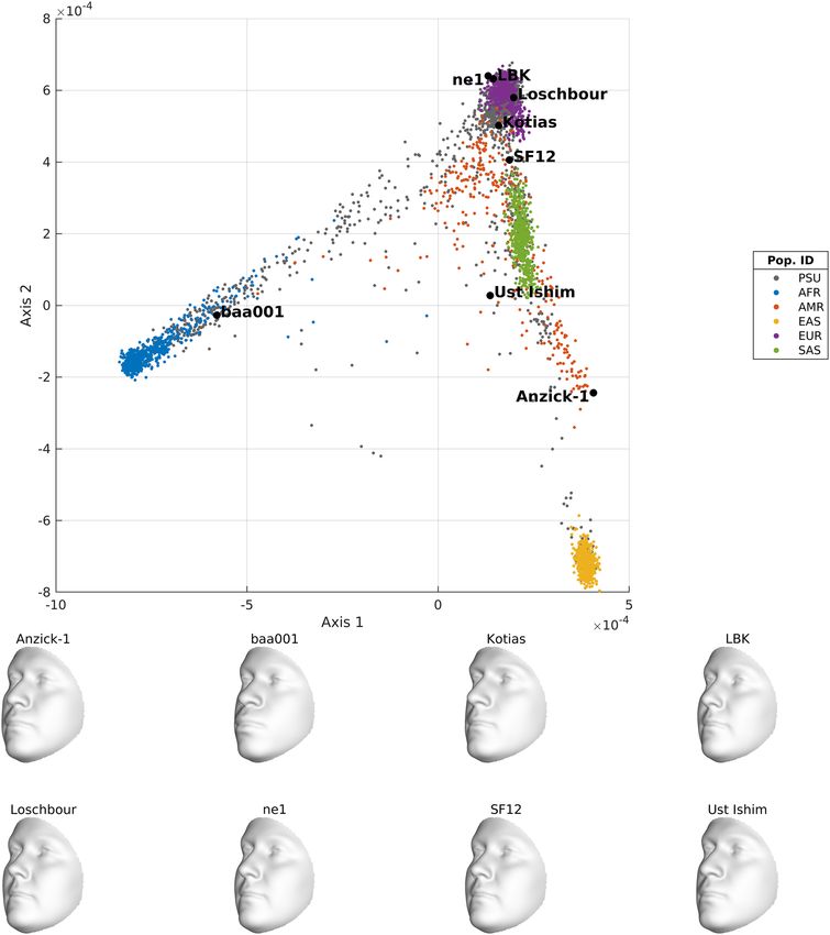
www.nature.com/scientificreports/
can be used to infer the population structure of samples with family structure or cryptic r elatedness1 and to inves-
tigate the genetic similarity between ancient DNA and modern human g enomes6. They also have the potential
to correct for population structure in a genome-wide association study (GWAS) on heterogeneous and admixed
samples. Of final interest is the association of auxiliary data (e.g. specific phenotypes, such as 3D facial shape
used in this work) present in internally collected datasets with ancestral variations captured by a reference space.
This requires the projection of the collected datasets into a reference space, followed by an association of the
projection scores with the auxiliary data presented.
Methodologically, the idea is to construct an ancestry latent-space from a reference dataset and to enable the
projection of new cases from other datasets that follow the mainstream of the reference dataset. Starting from
genome-wide single nucleotide polymorphisms (SNPs), principal component analysis (PCA) and analogous
dimension reduction techniques on normalized genotype data are popular strategies used in this c ontext7,8.
However, in construction of an ancestry space, these approaches are known to be sensitive to o utliers7,9. In addi-
tion and more importantly, in projecting new cases onto an ancestry space, PCA produces patterns of misalign-
ment (for example, “shrinkage” patterns where projected cases tend to falsely gravitate towards the center of the
ancestry space) due to missing data, missing heterozygotes, and genotyping along with imputation errors, which
is misleading without careful interpretation1. Therefore, stringent quality control and data filters are typically in
place to remove individual outliers and SNP data with high missing rates or not in Hardy–Weinberg equilibrium
(HWE). However, in heterogeneous datasets, in contrast to homogeneous datasets, such data filters are harder to
define, and potentially remove SNP data related to population structure. Furthermore, genotyping and imputa-
tion batch artefacts, not detected by quality control and different from one protocol to another, typically remain
and still affect an integrative analysis of ancestry.
In this work, we propose a novel robust genome-wide ancestry inference (referred to as SUGIBS) based on the
spectral (S) decomposition of an unnormalized genomic (UG) relationship matrix generalized by an Identity-by-
State (IBS) similarity degree of individuals’ matrix. Robustness against outliers during ancestry space construc-
tion, is obtained by absence of specific sample statistics (e.g. allele frequencies). Furthermore, SUGIBS provides
a robust projection of new samples, from different studies, onto a reference SUGIBS space. During projection,
the IBS similarity degree of unseen individuals to individuals in the reference dataset acts as a correcting term
for missing genotypes and errors, and most interestingly this correction is on an individual-by-individual basis.
We test the robustness of SUGIBS and compare its performance to PCA and Multi-Dimensional Scaling (MDS)
in revealing the underlying structure of an admixed population and adjusting for false positive findings in a
simulated case–control admixed GWAS. Using the 1KGP as reference dataset, and an additional heterogeneous
dataset containing 3D facial images, we apply SUGIBS to integrate the different datasets and combine this with a
shape regression to construct average faces that illustrate the ancestral variations captured within the 1KGP. We
further integrate eight ancient DNA profiles, which typically present higher genotyping error rates compared to
modern DNA, and reconstruct their ancestry-derived average faces. Based on the results, our method facilitates
a robust integrative analysis for ancestry estimation in heterogeneous datasets.
Results
Reference ancestry spaces with individual outliers. In the first experiment, we investigated the
robustness of SUGIBS in comparison to traditional approaches, in particular PCA using normalized or unnor-
malized genotype data and MDS using IBS distances as they are implemented in PLINK 1.910, against individual
outliers in a reference dataset. For this purpose, we first selected all unrelated individuals from the CEU and TSI
populations in the HapMap 3 project3 and used SUGIBS, PCA, unnormalized PCA (UPCA) and MDS to illus-
trate the first and second latent dimensions as ancestry components (Fig. 1, top row). In contrast to the tradition-
ally used normalized genotypes in PCA, UPCA used unnormalized genotypes that were not centralized around
the mean and were not standardized to a variance equal to one. As expected, PCA, MDS and SUGIBS are able to
differentiate between both populations along the first ancestry component. UPCA differentiates between both
populations along the second ancestry component, with the first aggregating an average SNP pattern, which is
common when running PCA on non-centered data. Surprisingly, with PCA a single outlier (NA11917) that was
not expected during the selection of both populations already affected the second ancestry component. Subse-
quently, we randomly selected one individual from four different and additional populations (CHB, GIH, MEX
and YRI) as “true outliers” in the dataset. Figure 1, bottom row, illustrates the first two ancestry components of
the four methods constructed on the dataset with outliers, where all four approaches clearly separate the outliers.
Using PCA, in contrast to MDS, UPCA and SUGIBS the clear distinction between CEU and TSI is lost within the
first two ancestry components, as they mainly capture variations due to the outliers. The main reason for robust-
ness in UPCA, MDS and SUGIBS is that these three methods use unnormalized genotype data and therefore
do not rely on specific sample statistics (e.g. allele frequencies), that otherwise increase the influence of outlier
variation. The single outlier (NA11917) in Fig. 1(A) using PCA disappears when true outliers were added to the
data in Fig. 1(E). This indicates that the population label CEU of individual NA11917 is most likely correct in the
context of variation present from multiple populations. Therefore, NA11917 is likely a false outlier, potentially
due to small errors in the data of this individual, but this is harder to verify.
Robust projection of unseen individuals onto reference ancestry spaces. In a second experiment,
we projected (“Methods”, Eq. 4) new samples on an ancestry space, based on the 1KGP as reference dataset, to
investigate the robustness of SUGIBS in comparison to PCA and UPCA against typical artifacts of different labo-
ratory protocols. Note that, since the first component of UPCA just aggregated the average SNP pattern as seen
in experiment 1, we started UPCA from the second component onwards. MDS does not allow for a straight-
forward projection of new samples on a reference space and was therefore excluded. As samples to project,
Scientific Reports | (2020) 10:11850 | https://doi.org/10.1038/s41598-020-68259-w 2
Vol:.(1234567890)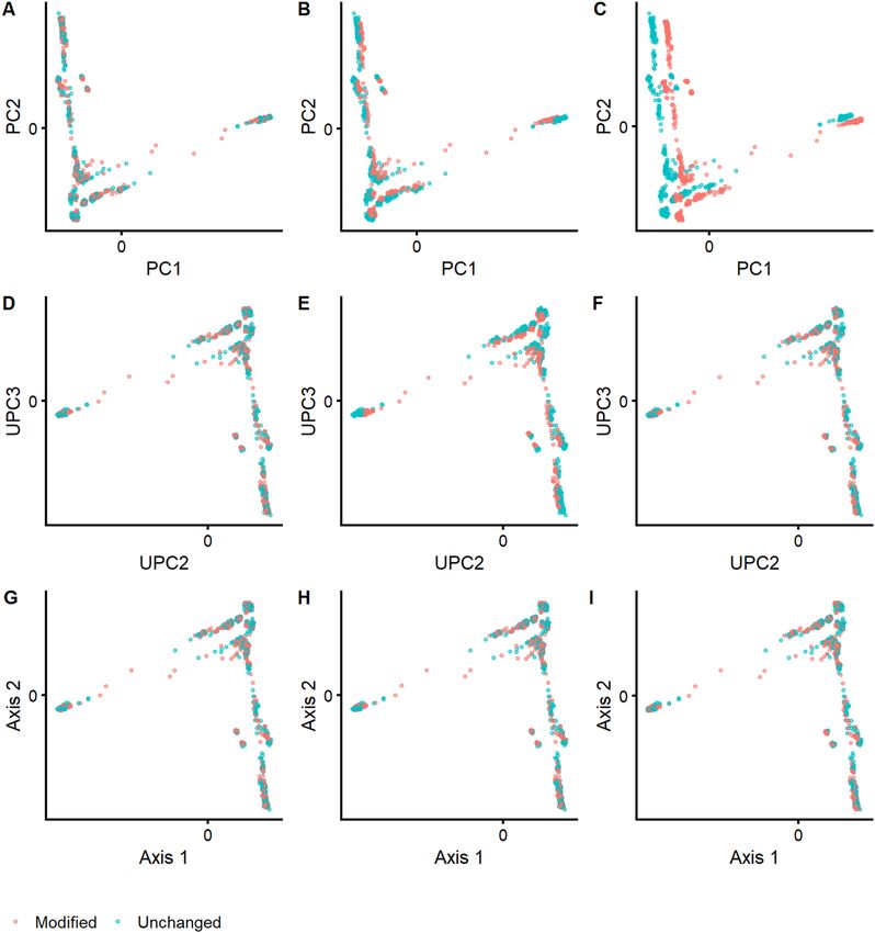
www.nature.com/scientificreports/
Figure 1. Robustness against individual outliers during the construction of an ancestry space. Top row, the
first two ancestry components for (A) PCA, (B) MDS, (C) UPCA and (D) SUGIBS using the CEU and TSI
populations from the HapMap 3 project. Bottom row, the first two ancestry components for (E) PCA, (F)
MDS, (G) UPCA and (H) SUGIBS using the CEU and TSI populations from the HapMap 3 project, but with
randomly selected single individuals from four different and additional populations (CHB, GIH, MEX and YRI)
as “outliers”.
we randomly assigned all 1,043 individuals of 51 populations from the HGDP dataset4 into two equally-sized
samples, one unchanged and one modified, respectively. To investigate the influence of different rates of missing
data, we randomly masked 5% of the SNP genotypes as missing in the modified dataset (See “Methods”). For the
influence of different rates of errors, we partially changed SNP genotypes with minor allele frequency (MAF) less
than 5% in the modified dataset (See “Methods”). Note that this was done knowing that more imputation errors
are observed in SNPs with a MAF of 5% and less11. We projected both HGDP datasets onto the PCA, UPCA
and SUGIBS reference spaces as defined by the 1KGP. In PCA, the simulated artefacts generated “shrinkage” and
“shifting” patterns of misalignment in the first two projected ancestry components (Fig. 2, top row), for missing
and erroneous genotypes, respectively. UPCA was only influenced by missing genotypes (Fig. 2, middle row).
In contrast, SUGIBS was not influenced by missing or erroneous genotypes (Fig. 2, bottom row). Figure 3 sum-
marizes the normalized root-mean-square deviations (NRMSD) of the first eight axes of SUGIBS, UPCA and
PCA of the modified HGDP dataset over 100 simulations. SUGIBS is significantly more robust than PCA in the
presence of missing and genotyping/imputation errors in new data for which ancestry needs to be inferred, by
projecting it into a reference space.
Revealing and adjusting for population structure in an admixed population. In a third experi-
ment, we investigated the ability of SUGIBS compared to PCA and MDS in representing admixture, since both
are commonly used in practice. UPCA on the other hand is not commonly used. However, it shares a strong
overlap with SUGIBS in starting from unstandardized genotypes, and therefore the results of UPCA are not
reported here since they corroborate perfectly with those of SUGIBS. Following the work of Galinsky et al.12, we
simulated data at 3,200 random independent SNPs for 200 individuals from a recent admixture of two popula-
tions, 50% from each population on average with divergences Fst = {0.001, 0.005, 0.01, 0.05, 0.1}, from an intra-
European difference to an intercontinental difference13. Because the admixture contains only one dimension of
population structure, only the first component of variation is of interest. Figure 4 presents the absolute correla-
tions between the first component of PCA, MDS and SUGIBS and the simulated ancestry proportions over 100
runs. When the Fst divergence between two populations is lower than 0.05, the correlation between the SUGIBS
component and the ancestry proportion is similar to that of MDS, but a little lower than PCA. We noticed that
when Fst ≤ 0.01, all three methods have a reduced performance to reveal the underlying admixture and when
Fst > 0.01, all three methods perform perfectly. According to the work of Patternson et al.8, the theoretical finest
divergence between two isolated populations, which can be detected by this amount of SNPs and samples would
be Fst = √3200×200/2
1
≈ 0.002. In line with this theoretical boundary, our results show that for Fst = 0.001, all
methods hardly detected any structure. At Fst = 0.005, all three methods start to detect population structure
(|r| > 0.7).
Following the work of Price et al.14, we also simulated a case–control GWAS to investigate if the population
structure inferred by SUGIBS can be used for correcting population stratification as a confounder. Only low
divergences between the two populations Fst = {0.001, 0.005, 0.01}, were tested, because for larger divergences
all three methods would perform the same as deducted from the previous experiment. Tests were conducted
Scientific Reports | (2020) 10:11850 | https://doi.org/10.1038/s41598-020-68259-w 3
Vol.:(0123456789)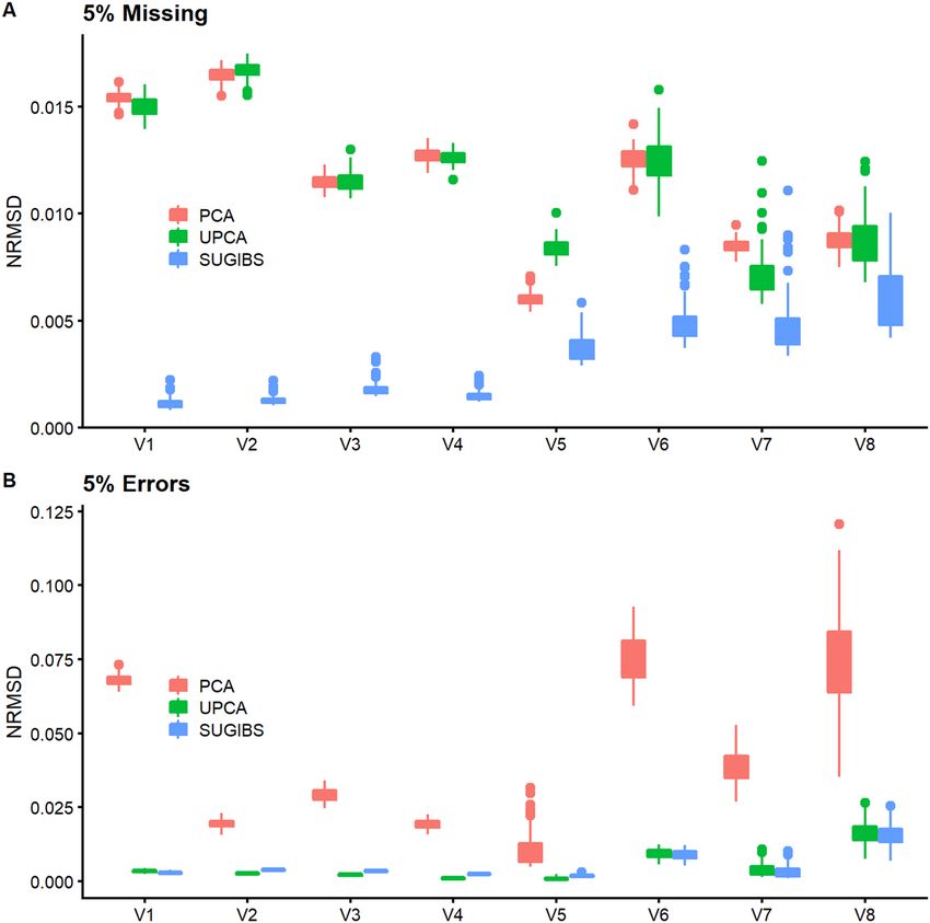
www.nature.com/scientificreports/

                                      Figure 2.  Robustness against batch artefacts during the projection of two distinct HGDP data partitioned
                                      samples, one to modify (pink) and one to remain unchanged (blue), onto a 1KGP based reference ancestry
                                      space. First Column, (A), (D), and (G), no real modification of the genotypes was done whereby both data
                                      partitions, pink and blue, overlap perfectly for PCA, UPCA and SUGIBS, respectively. Second column, (B), (E),
                                      and (H), a first actual modification was done by introducing missing genotypes in the data of the partition to
                                      modify (pink) with results for PCA, UPCA and SUGIBS, respectively. Third column, (C), (F), and (I), a second
                                      actual modification was done by modifying genotypes in the data of the partition to modify (pink) with results
                                      for PCA, UPCA and SUGIBS, respectively.

                                      with a logistic regression under four different correction scenarios: (1) no population for stratification correc-
                                      tion (Naïve), (2) PCA, (3) MDS and (4) SUGIBS, using a likelihood ratio test for the significance of each genetic
                                      marker. The experiment was conducted 100 times, using 1 million SNPs on 1,000 individuals, with average
                                      proportions of SNPs detected as significant shown in Table 1. These results indicate that in a single dimensional
                                      population structure, correcting using MDS, SUGIBS and PCA perform similarly, both in terms of Type I error
                                      and power. All three methods failed to correct the population stratification when Fst = 0.001, which is consistent
                                      with the failure of the three methods in revealing the admixture structure in the previous experiment. Finally,
                                      these results are in line with the results in the work of Price et al.14.

                                      Practical illustration of genome data integration using 3D facial images.                    Putting SUGIBS to
                                      practice in integrating multiple datasets, we projected 2,882 unrelated individuals from a large admixed and
                                      heterogeneous dataset containing individuals from varying ancestries (the PSU cohort, see Methods) and eight
                                      famous ancient DNA samples onto the first 25 SUGIBS axes established from the 26 populations in the 1KGP.
                                      Using the first eight SUGIBS scores of the PSU cohort onto the ancestry components of the 1KGP, we fitted a
                                      partial least squares regression (PLSR) to model facial variations in function of each of the first eight ancestry
                                      components. Shown in Figs. 5 and S1–5(a), the first two ancestry components separate the African (AFR) and
                                      East Asian (EAS) populations from the remaining populations, as indicated by the population labels given in

          Scientific Reports |   (2020) 10:11850 |              https://doi.org/10.1038/s41598-020-68259-w                                             4

Vol:.(1234567890)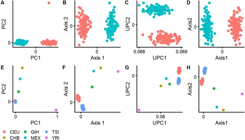
www.nature.com/scientificreports/
Figure 3. Normalized root-mean-square deviation (NRMSD) of the top eight axes of PCA, UPCA and
SUGIBS. NRMSD measures the root-mean-square differences (RMSD), for the modified HGDP dataset only
between the scores on ancestry axes generated using the original genotypes (error free) and the modified
genotypes (with simulated errors, A) missing genotypes and (B) erroneous genotypes). The RMSD values were
normalized by the range of the ancestry axes generated using the original genotypes, so that NRMSD of the
three methods (PCA, UPCA and SUGIBS) are comparable.
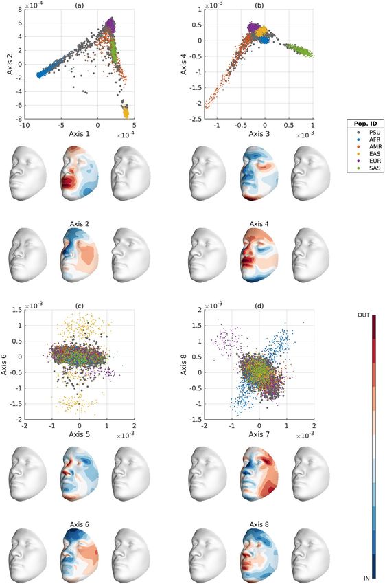
the 1KGP. The next two ancestry components in Figs. 5 and S1–5(b) separate the South Asian (SAS) population
and visualizes the admixture in the Admixed American (AMR) population, respectively. In Figs. 5 and S3(c),
the sixth ancestry component captures different subpopulations in the EAS population. In Figs. 5 and S1(d), the
seventh ancestry component is driven by African subpopulations. The separated European subpopulation on
the eighth ancestry component is the population from Finland (FIN), Fig. S4(d). The projected PSU cohort is
indicated by gray dots in Figs. 5 and S1–5 and overall it is observed that they overlay well with a wide range of
ancestry variations in the 1KGP confirming the heterogeneous and admixed nature of the PSU dataset. However,
some populations in the 1KGP are less covered by the PSU cohort, such as the population of Finland in Europe
and some African subpopulations on ancestry components seven and eight (Fig. 5d).
Based on the visually strong and recognizable human facial phenotype, we generated comprehensive illus-
trations of the population structure embedded in the 1KGP. In Fig. 5, strong facial differences are observed for
ancestry components 1–4, whilst perceptually smaller differences occur in components 5–8. This is most likely
due to a lower overlap of the PSU cohort with these ancestry components. i.e. the PSU cohort captures the vari-
ation across the larger continental population groups, but not the variation at the finer intra-continental popu-
lation level. Finally, in integrating additional data sources from ancient DNA into the same ancestry space we
derived an ancestry-driven average facial representation for eight high-coverage ancient DNA profiles (Fig. 6).
It is observed that their projections within the 1 KGP ancestry space is consistent with the intercontinental
geographical locations where these samples were discovered and what is currently known about these samples
(Supplementary Table S1).
Scientific Reports | (2020) 10:11850 | https://doi.org/10.1038/s41598-020-68259-w 5
Vol.:(0123456789)
www.nature.com/scientificreports/
Figure 4. Capturing simulated admixture in function of Fst. X-axis represents the different levels of Fst
investigated. The Y-axis represents the absolute correlation of the first component in PCA, MDS and Spectral-
IBS with the simulated ancestry proportion. The higher the correlation the better a method is able to capture the
underlying admixture.
Naive PCA MDS SUGIBS
F st = 0.001
Random 0.0002 0.0001 0.0001 0.0001
Differentiated 0.9960 0.4483 0.6370 0.5200
Causal 0.5295 0.4779 0.4865 0.4807
F st = 0.005
Random 0.0009 0.0001 0.0001 0.0001
Differentiated 0.9980 0.0002 0.0003 0.0002
Causal 0.5226 0.4249 0.4255 0.4253
F st = 0.01
Random 0.0030 0.0001 0.0001 0.0001
Differentiated 0.9971 0.0001 0.0001 0.0001
Causal 0.5166 0.4227 0.4230 0.4229
Table 1. Proportion of associations reported as statistically significant (P < 0.0001) by logistic regression
using a likelihood ratio test. Random SNPs with no association to the disease were generated by simulating
random drift with Fst divergence. Differentiated SNPs with no association to the disease were generated by
assuming population allele frequencies of 0.8 of ancestry 1 and 0.2 of ancestry 2. Causal SNPs were generated
by combining a multiplicative disease risk model while simulating the random drift with the same Fst as the
random SNPs. See methods for more details on the parameters.
Discussion
Accurate inference of population structure and individual global ancestry is of critical importance in human
genetics, epidemiology, and related fi elds15,16. The analysis of population structure in itself can yield significant
insights in terms of population dynamics, both in modern and ancient populations17–19. Through inspection of
ancestry components as well as distances in genetic latent spaces created by, for example, principal component
analysis (PCA), it is possible to infer patterns of gene flow and population movements through time. Further-
more, The inclusion of various populations in genome-wide association studies (GWAS) could increase statisti-
cal power and make better contributions to our understanding of the genetics of complex traits for the human
population as a w hole20. However, the widely used approach of PCA and analogous techniques are sensitive to
outliers, when constructing ancestry spaces, and produce patterns of misalignment due to artifacts of different
laboratory protocols when new samples are projected onto a reference ancestry s pace1,7,9. We propose a robust
alternative for genome-wide ancestry inferencing, referred to as SUGIBS. Our results confirm the erroneous influ-
ences in PCA based ancestry estimations that are misleading without careful interpretation. In constructing an
ancestry space, SUGIBS shares the same robustness against individual outliers as MDS or related spectral graph
approaches21. Furthermore, and more importantly, during dataset projections SUGIBS is robust against typical
artefacts from different laboratory protocols. In addition, SUGIBS achieved almost the same performance, under
Scientific Reports | (2020) 10:11850 | https://doi.org/10.1038/s41598-020-68259-w 6
Vol:.(1234567890)www.nature.com/scientificreports/
Figure 5. Top eight SUGIBS axes of 1KGP and projections of the PSU cohort. (A) The first (horizontal) and second (vertical)
axes. (B) The third (horizontal) and fourth (vertical) axes. (C) The fifth (horizontal) and sixth (vertical) axes. (D) The seventh
(horizontal) and eight (vertical) axes. Grouped populations of the 1KGP are coloured dots (AFR, African, AMR, Admixed
American, EAS, East Asian, EUR, European, SAS, South Asian). The projected PSU cohort are represented by grey dots.
The faces illustrate opposing variations along each of the ancestry components and are not associated to any of the 1kG
populations in particular. For each axis, we visualize a face − (left) and + (right) 3 times the standard deviation (sd) from the
1KGP mean on that axis. In the middle, the blue-red colormap highlights inward (blue) and outward (red) facial difference
going from the + 3 sd to the − 3 sd facial gestalts. The values for sex, height, weight and age were 1.5 (genderless), 165 cm,
75 kg and 30 years, respectively.
Scientific Reports | (2020) 10:11850 | https://doi.org/10.1038/s41598-020-68259-w 7
Vol.:(0123456789)www.nature.com/scientificreports/
Figure 6. Ancestry-derived facial averages based on eight ancient DNA profiles. For these facial averages,
the sex (1 for male, 2 for female) was known from the DNA profile and taken into account in the partial least
squares regression model. The values for height, weight and age were 165 cm, 75 kg and 30 years, respectively.
error-free conditions, as PCA in revealing the underlying structure of an admixed population and avoiding false
positive findings in a simulated case–control GWAS with an admixed population.
Irrespective of the method of choice, two general notes apply here. First, as with MDS and PCA, there is a
range of possible population histories that could generate the same pattern in SUGIBS. For example, a gradient
including multiple individuals could be interpreted as the result of gene flow, admixture or isolation-by-distance.
In such situations, it is important to see methods like PCA and SUGIBS as exploratory analysis only to gener-
ate hypotheses which can and should be formally tested using additional approaches (e.g. f statistics for gene
flow and admixture22). Second, although detecting and adjusting for population stratification in closely related
populations and hybrids of these are more difficult than for populations that show more differentiation (higher
Fst), there are important questions regarding how much such stratification can affect studies performed in what
are considered "homogeneous" populations with respect to admixture; in other words, cryptic stratification23. It
will also be important to understand how well cryptic stratification can be controlled by the various methods as
a function of minor allele frequency, i.e., rare SNP vs. common S NP23.
Like MDS and SUGIBS, PCA is also a “spectral” method, in which the edge similarity between individuals
is simply the covariance of normalized genotypes, commonly referred to as the genomic relationship matrix24.
Scientific Reports | (2020) 10:11850 | https://doi.org/10.1038/s41598-020-68259-w 8
Vol:.(1234567890)www.nature.com/scientificreports/
However, this covariance similarity used in PCA depends on the allele frequencies as a non-robust sample sta-
tistic to normalize the genotypes, which causes sensitivity to individual outliers. Note that in our experiments
on PCA without using allele frequencies (UPCA) robustness against individual outliers was observed. Among
the “spectral” methods, some other robust alternatives were introduced to infer population structure, including
a modified genomic r elationship21,25. MDS or related spectral graph approaches21 using IBS and Allele Sharing
Distance (ASD) similarities between individuals (available in PLINK10) are also a robust alternative against indi-
vidual outliers, as illustrated in our results. IBS and ASD are unnormalized distances, and thus less influenced by
outliers. However, MDS and the modified genomic relationship21,25, both lack the ability to project new samples
on an already established reference ancestry space. Alternatively, it might be possible to use one of the many
robust PCA approaches that have been investigated for general d ata26–28 as well as genetic d
ata29. However, in most
study data processing protocols, robust approaches are usually used for outlier detection rather than inferring
population structure, which is done by classical PCA after excluding outliers29. This is for example, a standardly
used option in the popular EIGENSOFT software7. Note that, when establishing an ancestry space from a refer-
ence dataset, it remains good practice to identify and remove individual outliers, if they are of no further interest.
The main contribution of SUGIBS is robustness against batch artifacts of different laboratory and data pro-
cessing protocols when projecting new samples onto a reference ancestry space. In the case of missing genotypes,
smaller absolute PC scores, and smaller UPC scores are wrongfully generated during the projection of samples.
These smaller and decreased scores lead to the “shrinking” and “shifting” patterns as observed in the results. (Note
that this is not to be confused with PCA shrinkage due to high dimensional and large-scale data, which is dealt
with using shrinkage eigenvalue estimations as recently implemented in EIGENSOFT). However, to correct for
this, the projected SUGIBS score matrix is weighted by the reference degree matrix, which captures the similarity
between the data to be projected and the reference data (see “Methods”). This weighting of projected SUGIBS
scores equally corrects for the effects of genotyping and imputation errors, as demonstrated in the results. To the
best of our knowledge, we are currently not aware of another related approach that offers the same robustness.
Based on the results, we argue that SUGIBS is a solid alternative to PCA and MDS and requires less stringent data
filters to operate. Our implementation of SUGIBS uses the randomized singular value decomposition a lgorithm30,
that is also used in F astPCA12. This makes the algorithm computationally tractable for datasets with tens of
thousands of individuals and millions of SNPs. E.g. the calculation of the loadings for eight components based
in 6,000 individuals using 300,000 SNPs takes two minutes compared to one hour using a standard singular value
decomposition on a Mac Pro (Late 2013), Intel Xeon CPU E5-2697 v2 @ 2.70 GHz (12 core), 64.00 GB 1,600 MHz
DDR3. SUGIBS is available as part of an open-source in-house matlab library, referred to as SNPLIB, in which we
used PLINK binary file formats as input, and provide FastPCA, logistic GWAS and all other methods, including
the simulations mentioned throughout this work. Furthermore, SUGIBS can easily be incorporated into exist-
ing and interesting extensions to derive common ancestry estimations in datasets with non-overlapping genetic
variants1, or genotyping-by-sequencing data31, or population structure inference in presence of relatedness32, or
in iterative schemes to obtain global to fine-scale ancestry e stimations33.
There are a few points of discussion and future investigations. First, a genetic similarity measure between pairs
of individuals aims to identify how they are related and different measures exist for ancestry estimations (e.g.
IBS, ASD, Identity-by-descent, normalized covariance)24. Commonly used similarity measures are normalized,
just like the traditional approach of PCA on normalized genotype data, to take the genetic composition of indi-
viduals along with the rest of the sample into account. A normalization does have the advantage that individuals
within the same population are more similar to each other than to individuals in other p opulations24. In other
words, the distinction between populations increases, which improves population identification by clustering
algorithms. However, when the normalization is performed incorrectly clustering efforts might be inaccurate.
Furthermore, as seen in our results, such a normalization increases the influence of individual outliers. Finally,
in contrast to homogeneous datasets, normalization of genotype data in heterogeneous datasets is challenging
depending on whether the dataset is unlabeled or not, imbalanced or not, and with high admixture or not.
Starting from unlabeled data, unsupervised clustering approaches such as A DMIXTURE34 and STRUCTURE35,
iteratively identify the populations individuals belong to and update the normalization accordingly. However, this
involves additional parameters to set and tune, the most important one being the amount of clusters expected
in the data. Without prior knowledge on how to set these parameters, this can turn into a challenging task.
With highly admixture data, any clustering of global ancestry into populations is even questionable. In these
situations, only local ancestry estimations, using chromosome painting a pproaches36 for example, are meaning-
ful. Alternatively, in the future, we want to investigate the use of a reference ancestry space as constructed in
this work, without assigning individuals to specific populations, in estimating normalized genotype data on
an individual-by-individual basis. I.e., an ancestry space from unnormalized genotype data is a good first step
unbiased by any sample statistics, to further deduct statistics related to individual genotype profiles. For example,
Kwong et al.37 propose the Robust Unified Test for Hardy–Weinberg Equilibrium in the context of an admixed
population, which also makes use of individual-level adjustments for ancestry. Second, future investigations of
the methodology also include the influence of Linkage Disequilibrium (LD) pruning and data filtering for SNP
selection. Population admixture is one of the main sources for LD between SNPs, therefore we prefer to avoid
excessive LD pruning before applying SUGIBS. As stated in Lawson and F alush24 any data pruning or filtering
is bound to loose information related to population structure. For example, less common variants are typically
lost in data filtering, but these might contain valuable information about population s tructure24. Since SUGIBS
is robust and computationally tractable, any data filtering can be minimized. Third, another future investigation
involves the determination of the number of relevant or significant components in SUGIBS, for which we provide
a preliminary suggestion that compares the spectrum of the data observed with that of a simulated homogenous
dataset assuming linkage equilibrium (LE) and Hardy–Weinberg Equilibrium (Supplementary Note S1).
Scientific Reports | (2020) 10:11850 | https://doi.org/10.1038/s41598-020-68259-w 9
Vol.:(0123456789)www.nature.com/scientificreports/
We recommend the following procedure to extract a common set of SNPs between a reference dataset and
another dataset being projected, for constructing SUGIBS ancestry spaces. First, exclude all the indel, mono-
morphic, and multi-allelic SNPs in both the reference dataset and the dataset to project. Subsequently, extract
the list of SNPs common in both datasets. Based on this list, we further recommend a minor allele frequency
(MAF) filtering with a MAF threshold of 1% on the reference dataset using PLINK10 as a quality control step. We
do not recommend Hardy–Weinberg disequilibrium (HWD) filtering since it is probably the result of popula-
tion admixture and thus useful for our purposes38. Although population admixture is one of the main sources
for LD between SNPs, we still recommend LD pruning since it is not unusual to have non-uniformly genotyped
genomes. Similar to PCA, SUGIBS does not explicitly model LD between SNPs so that misleading results might
be generated without LD pruning.
In application of SUGIBS we used the human face, which is a powerful phenotype to visualize and illustrate
underlying genetic ancestry variations. Indeed, faces are easy to recognize, interpret, and validate the outcomes
based on everyone’s expert knowledge in facial perception. The faces illustrating the variation in ancestry compo-
nents of the 1KGP in this work overlay well with the 1KGP super population labels that represent intercontinental
differences. Facial variations at the level of intracontinental populations were perceptually harder to observe,
mainly due to a lack of overlap of the PSU cohort with many of the 26 1KGP subpopulations. We further used
SUGIBS to integrate eight ancient DNA profiles into the 1KGP ancestry space. Despite many advances in ancient
DNA methodologies, DNA extracted from archaeological remains is usually associated with higher error rates
than modern DNA. Over time, different biochemical processes cause a degradation of the DNA molecules lead-
ing to short f ragments39 that increase the chances of mapping errors. Furthermore, post-mortem deamination of
cytosine into uracil is generating false cytosine to thymine changes after PCR and sequencing which increases the
per-sample error rate40. Furthermore, handling of human remains by other human individuals comes with the
inherent risk of modern human contamination which can be seen as another source of errors introduced into the
DNA sequence of the ancient individual. Therefore, even though any other method, such as PCA, can be used in
a shape regression framework to generate average ancestry 3D faces, SUGIBS provides a “piece of mind” against
the inevitable presence of genotyping errors and missing data as illustrated throughout the results. Finally, it is
important to note that an ancestry-derived face are not individually specific faces, but average faces that simply
visualize the ancestry background of a DNA profile. Related work on facial prediction from DNA41,42, also show
that sex and ancestry are primary factors driving the estimation of facial shape from DNA. Further information
on the potential value of ancestry-derived faces is provided in Supplementary note S2.
In conclusion, SUGIBS is a novel approach to construct an ancestry space from a reference dataset and to
project new samples from heterogeneous datasets for a consistent and robust inference of individual ancestry.
The main contributions involve robustness against outliers during the construction of an ancestry space, and
robustness against batch artefacts during the projection of new samples into an ancestry space. Therefore, SUGIBS
is a solid alternative to PCA and MDS and facilitates a robust integrative analysis for population structure and
ancestry estimations for heterogeneous datasets. Based on the visually strong and recognizable human facial
phenotype, comprehensive illustrations of genomic ancestry related variations within the 1KGP and for eight
ancient-DNA profiles were provided.
Materials and methods
SUGIBS reference‑space. Given a dataset with N individuals and M SNPs, we first create an unnormal-
ized genotype (UG) matrix X M×N with additive genotype coding (aa = − 1, Aa = 0, AA = 1 and missing = 0). The
UG relationship matrix is then defined as G = M1 X T X . From W N×N , the IBS similarity matrix of the same
dataset used to create G , the similarity degree of an individual can be defined as dii = N
j=1 wij . We followed the
algorithm implemented in PLINK to calculate the IBS similarity so that:
IBS AA Aa aa
AA 2 1 0
Aa 1 2 1
aa 0 1 2
N/A 0 0 0
However, in contrast to the calculations in PLINK, we do not normalize the IBS similarity matrix with miss-
ingness scores. This results in a similarity degree matrix D defined as the diagonal matrix with d11 , . . . , dNN on the
diagonal. We use D to define generalized eigenvectors v k = (vk1 , . . . , vkn )T of G with corresponding generalized
eigenvalues k , and 1 ≥ 2 ≥ 3 ≥ · · ·:
Gv k = k Dv k (1)
Similar to PCA on non-centered or unnormalized data, the first generalized eigenvector of D and G simply
represents the average pattern of all SNPs (see Fig. 1). Therefore, we start from the second generalized eigenvector
and define the k th component
1
of SUGIBS to be the k + 1th generalized eigenvector of G and D , v k+1.
By multiplying D− 2 on both sides of Eq. (1), we obtain:
1 1 1 1
D− 2 GD− 2 D 2 v k = k+1 D− 2 v k (2)
1 − 12 − 21
′ − 12 − 21
Subsequently, we observe that the eigenvector v k = D v k of D GD
2
1
= M1 D X T XD can be obtained
from the singular value decomposition (SVD) of the matrix X̂ = XD− 2 = U V ′T , where v k is also the i th right
′
Scientific Reports | (2020) 10:11850 | https://doi.org/10.1038/s41598-020-68259-w 10
Vol:.(1234567890)www.nature.com/scientificreports/
singular vector with singular value σk = M k+1 , is a N × N diagonal matrix, U is a M × N matrix with all
the left singular vectors
and V is a
N × N matrix with
′
all the right
singular vectors.
Denoting U k = u2 , . . . , uk+1 and k = diag σ2 , . . . , σk+1
1
, the corresponding
′ 1
left
singular vectors and
the singular values of the first k SUGIBS components V k = D− 2 V k = D− 2 v 2 , . . . , v k+1 , we have the follow-
ing equation:
1
V k = D− 2 V ′k = D−1 Sk = D−1 X T Lk = D−1 X T U k k−1 (3)
Thus, we denote Lk = U k −1
k as the SUGIBS loading matrix for the first k SUGIBS components and
Sk = X T U k −1
k as the unnormalized SUGIBS score matrix.
SUGIBS dataset projection. Given the ∼ SUGIBS loadings Lk from a reference dataset with N individuals
and M SNPs and given a new dataset with N individuals and the same ∼
set of SNPs as the reference sample, we
denote the∼ unnormalized
∼ ∼
genotype matrix of the new dataset as X . We then define the reference degree
N
d ii = j w ij , where w ij is denoted as the IBS similarity between the i th individual ∼
in the target dataset and the
j th individual in the reference dataset. The reference similarity degree matrix D of the new dataset is a diagonal
∼ ∼
matrix with d 11 , . . . , d ∼ ∼ on the diagonal. For the first k SUGIBS components, the projected score matrix of the
NN
target dataset is then obtained as:
−1 −1 T −1 T
Ṽ k = D̃ S̃k = D̃ X̃ Lk = D̃ X̃ U k −1
k (4)
∼
In Eq. (4), the reference similarity degree matrix D acts as a normalization term correcting the missing
genotypes and errors in the samples to be projected. As an example, consider a rare SNP with major allele A
and minor allele G, and an individual with true genotype AA that is wrongfully coded as GG for that particular
SNP. Since the major genotype in the reference data of this SNP is AA, the number of shared alleles of this SNP
between this individual to the majority of individuals in the reference dataset would reduce from 2 to 0. The
unnormalized genotype coding of this person also changes∼ from 1 to − 1. Thus, the influence of such∼a genotyp-
ing error on the unnormalized SUGIBS score matrix S k and the reference similarity degree matrix D are along
∼ −1
the same direction so that the final SUGIBS scores are corrected by D . Other typical batch artefact errors and
missing genotypes in the new dataset are corrected for in a similar way and, most interestingly, this correction
is provided on an individual by individual basis.
The following is a description of the data used for each of the three experiments. An overview of different
data filtering steps for each of the experiments is provided in Supplementary Table S2.
Experiment 1, individual outlier robustness. The basic dataset to investigate robustness against indi-
vidual outliers in a reference dataset consists of the individuals from the CEU population (111 individuals) and
the TSI population (102 individuals) from the HapMap 3 dataset3, after excluding non-founders. Individuals
with more than 10% missing genotypes were removed. Related individuals were identified using KING43 with
threshold 0.044, which is the threshold for 3rd degree relatives, after which one of each pair of related individu-
als was randomly removed. We randomly selected one individual as outlier from four other populations (CHB,
MEX, GIH, and YRI). These individuals specifically are NA18798 (CHB), NA19740 (MEX), NA21124 (GIH),
and NA19262 (YRI). After removing the monomorphic SNPs in each of these three datasets, we built SUGIBS,
MDS, UPCA and PCA spaces using 892,338 autosomal SNPs remaining in all three datasets. We intentionally
did not perform either minor allele frequency (MAF) filtering or HWE filtering on the SNPs since many rare
SNPs and SNPs violating HWE are due to the outliers and were therefore not checked for during the testing for
robustness.
Experiment 2, simulated laboratory artefacts. We used the 1,000 Genomes Project dataset (2,504
unrelated individuals from 26 populations) as the reference dataset to infer ancestry spaces. We used the HGDP
dataset that analyzed genomic data from 1,043 individuals from around the world as the dataset to project.
For both 1KGP and HGDP dataset, individuals with more than 10% missing genotypes were removed. For the
1KGP only, related individuals were identified using K ING43 with threshold 0.044, after which one of each pair
of related individuals was randomly removed. First, we remapped the HGDP dataset from the NCBI36 (hg18)
assembly to the GRCh37 (hg19) assembly using the NCBI Genome Remapping Service. We further performed a
LD pruning with a window size of 50, a moving step of 5 and a threshold r 2 > 0.2 for several times until no more
SNPS were e xcluded12. LD pruning is a common practice when using PCA. Therefore, we followed this addi-
tional step to make the results based on PCA, UPCA and SUGIBS comparable for this particular experiment.
Doing so, we selected 154,199 autosomal SNPs to construct the ancestry spaces. We then extracted the first eight
ancestry components from the reference dataset. After extracting the same set of SNPs in the HGDP dataset, we
took care to ensure that the alternate alleles were the same as in the reference dataset.
Since PLINK binary file format stores the genotypes of four consecutive individuals in a single byte, we
assigned one of every two “bytes” (four individuals) into dataset A (the dataset to modify) and the other indi-
viduals into dataset B (the dataset to remain unchanged) of the HGDP dataset. This resulted in 523 individuals
for dataset A and 520 individuals for dataset B. In order to simulate laboratory artefacts, we randomly masked
5% genotype calls as missing and changed 5% genotype calls (e.g., from AA to Aa or aa) of the rare SNPs
(MAF < 0.05) in dataset A. Random genotype masking and changing were also performed on the “byte” level,
i.e. four individuals at a time. For both genotyping masking and changing, we generated 100 datasets to project
on the 1KGP reference ancestry space. Subsequently, as input to Fig. 3, we calculated the root-mean-square
Scientific Reports | (2020) 10:11850 | https://doi.org/10.1038/s41598-020-68259-w 11
Vol.:(0123456789)www.nature.com/scientificreports/
deviations (RMSD) between the scores of the top eight ancestry axes generated using the original genotypes and
the modified genotypes in dataset A and further normalized them by the range of the axes generated using the
original genotypes so that normalized root-mean-square deviations (NRMSD) across methods are comparable.
Experiment 3A, simulated admixed population. Our admixture simulations were adapted from the
section “Simulation Framework” in Galinsky et al.12. 100 times we similated data at 3,200 random independent
SNPs for 200 individuals. For a given SNP i , the ancestral allele frequency pi was sampled from a Uniform(0.1, 0.9)
distribution. Population allele frequencies were generated by simulating random drift in two populations of fixed
effective size Ne for τ generations as pi1 and pi2, whose initial values were set to pi . In each generation, the num-
ber of alternate alleles zi1 and zi2 were sampled from two binomial distributions with 2N e number of trials and
pi1 and pi2 success probabilities. The population allele frequencies were then updated by pi1 = 2N zi1
e
and pi2 = 2N
zi2
e
.
For all simulations, population allele frequency simulations were run for 20 generations
and the effective popula-
τ 44
tion size Ne was calculated for a target Fst by Fst = −log 1 − 2N e
. This was done for
Fst = {0.001, 0.005, 0.01, 0.05, 0.1}, Ne ≈ {10k, 2k, 1k, 200, 100} with τ = 20.
The ancestry proportions αj were sampled from a beta(0.5, 0.5) distribution so that the proportion from each
ancestry
is 50% on average. For a given individual j with ancestry proportionj of αj from Population
one and
1 − αj from population two, the individual allele frequency for SNP i was pi = αj pi1 + 1 − αj pi2 and the
j
genotype was sampled from a binomial distribution with 2 trials and pi success probability.
Experiment 3B, simulated GWAS. Our GWAS simulation is similar to the one carried out in Price
et al.14. To simulate a case–control GWAS, we generated 1,000,000 SNPs for 1,000 individuals from a popula-
tion admixed from two ancestries. The case–control status was simulated using a disease risk proportional to r α,
based on an ancestral risk of r = 3. We generated three categories of SNPs (random, differentiating and causal)
to compare the performance of PCA, MDS, and SUGIBS in correcting for population stratification. For the first
category (random SNPs with no association to the disease), we generated the SNPs by simulating random drift
with a certain Fst divergence. For the second category (differentiated SNPs with no association), we assumed
population allele frequencies of 0.8 for ancestry one and 0.2 for ancestry two. For the third category (causal
SNPs), we generated SNPs by combining a multiplicative disease risk model while simulating the random drift
with the same Fst as the random SNPs.
We simulated the case–control status according to Price et al.7. For individuals with an ancestry propor-
tion of α from population one and (1 −a α) from population two, the case–control status was simulated with
the probability of disease equal to log(r)r 7
2(r−1) , which ensures an average value of 0.5 across all the values of α . For
the case individuals, the population allele frequencies pi1 and pi2 of the causal SNP i were further updated to
Rpi1 Rpi2
1−pi1 +Rpi1 and pi2 = 1−pi2 +Rpi2 with a relative risk of R = 3, respectively.
∗ =
pi1 ∗
PSU cohort and 3D facial images. Study participants in the PSU cohort were collected with informed
consent as part of several studies based at The Pennsylvania State University and sampled in the following loca-
tions: State College, PA (IRB #44929 & #4320); New York, NY (#45727); Urbana-Champaign, IL (#13103); Cape
Verde; Dublin, Ireland; Rome, Italy; Warsaw, Poland, and Porto, Portugal (#32341); and Twinsburg, OH (#2503).
The individuals were genotyped on the 23andMe v3 and v4 arrays (23andMe, Mountainview, CA) and Illumina
HumanHp200v1 BeadChip (Illumina Inc., San Diego, CA) platforms. After filtering out SNPs with more than
10% missing genotypes, the intersection of these two arrays compromised of approximately 600 K SNPs. We
removed individuals with misclassified sex information, missing covariate data, and those with more than 10%
missing genotypes. Relatives were identified as pairs of individuals using a KING43 with threshold (0.044, which
is the threshold for 3rd degree relatives), after which one of each pair was randomly removed, resulting in a set of
2,882 individuals. Genotypes were imputed to the 1,000 Genomes Project Phase 3 reference panel, using SHA-
PEIT2 for prephasing of haplotypes and imputed using the Sanger Imputation Server PBWT pipeline.
3D facial images were taken using the 3dMDface (3dMD, Atlanta, GA) and the Vectra H1 (Canfield, Parsip-
pany, NJ) imaging systems. Height and weight were measured using an Accustat stadiometer (Genentech, San
Francisco, CA), a clinical scale (Tanita, Arlington Heights, IL), or by self-report. 3D facial images were imported
into matlab 2016b in .obj wavefront format to perform spatially dense registration ( MeshMonk45). This resulted
in homologous spatially dense configurations of 7,160 quasi-landmarks per facial image. In other words, each 3D
image is represented with the same amount of 3D points that are in full one-to-one correspondence with all other
images. Reflected images were created by changing the sign of the x-coordinate of the original mapped images.
Both the original and the reflected remapped faces were then superimposed following a generalized Procrustes
superimposition to eliminate differences in orientation, position and scale46. Symmetrized images were created
by averaging the original and the reflected images.
Constructing ancestry‑derived average 3D faces. In total, we had 69,194 overlapping autosomal SNPs
that were present in the 1KGP dataset, the PSU cohort and the ancient-DNA profiles following a MAF filtering of
1%, HWE filtering with p-value threshold 1e-6, and LD pruning: window size, 50 step size, 5 and LD threshold of
0.2. Based on this selection, we constructed 25 SUGIBS ancestry components using the 1KGP dataset, which is
theoretically sufficient to separate 26 populations, from the 1KGP reference dataset. Subsequently, we projected
the 2,882 individuals from the PSU cohort and the eight ancient-DNA profiles onto the 1KGP ancestry com-
ponents using the same 69,194 overlapping autosomal SNPs. Then, we fitted a partial least-squares regression
(PLSR) model (plsregress function in matlab 2016b) using the superimposed and symmetrized 3D facial images
with 7,160 quasi-landmarks collected in the PSU cohort as the response variables, and the first eight projected
Scientific Reports | (2020) 10:11850 | https://doi.org/10.1038/s41598-020-68259-w 12
Vol:.(1234567890)www.nature.com/scientificreports/
SUGIBS scores of the PSU cohort together with four covariates [age (years), sex (1 = male; 2 = female), height
(cm) and weight (kg)] as the explanatory or predictor variables.
Given specific ancestry scores on the ancestry components of the 1KGP ancestry space, together with age,
height, weight and sex, the PLSR model was able to generate an ancestry-derived average face as response vari-
able. To illustrate the ancestry components in Fig. 5, we simply varied a single score along each ancestry compo-
nent separately, while keeping the scores on the other ancestry components fixed and equal to zero with following
values for age = 30 years, height = 165 cm, weight = 75 kg and sex = 1.5 (reflecting a genderless face). For example,
for the first axis in Fig. 5(a), the face along the positive direction of this axis was constructed using X = [30 1.5
165 75 mean (axis11kgp ) + 3*std (axis11kgp) 0 0 0 0 0 0 0] and the face along the negative direction of this axis was
constructed using X = [30 1.5 165 75 mean (axis11kgp) − 3*std (axis11kgp) 0 0 0 0 0 0 0]. The projected ancestry
scores of the eight ancient-DNA profiles were used together with the genome-derived sex values, age = 30 years,
height = 165 cm, weight = 75 kg as predictors in the PLSR model to construct the ancestry average 3D faces of
the respective ancient-DNA profiles.
Ethics statement. Institutional review board (IRB) approval was obtained at each recruitment site and
all participants gave their written informed consent prior to participation; for children, written consent was
obtained from a parent or legal guardian. For the PSU cohort, the following local ethics approvals were obtained:
State College, PA (IRB #44929 and #4320 New York, NY (IRB #45727); Urbana-Champaign, IL (IRB #13103);
Dublin, Ireland; Rome, Italy; Warsaw, Poland; and Porto, Portugal (IRB #32341); and Twinsburg, OH (IRB
#2503).
Consent for publication. All methods were carried out in accordance with relevant guidelines and regula-
tions.
Data availability
The data used to develop, validate and test SUGIBS in this work originates solely from public open-source pro-
jects, including the HapMap 3 project, 1,000 Genome project and the HGDP dataset. For access to this data, we
refer to their respective webpages as indicated under the URL section. An implementation of SUGIBS is freely
available (see URLs below). This comprises a matlab toolbox, referred to as SNPLIB, and contains implementa-
tions of all the methods and including the simulations used in this work. The data used to apply SUGIBS in
the context of facial shape variations was based on participants comprising the Penn State University dataset
(PSU cohort). However, these were not collected with broad data sharing consent. Given the highly identifiable
nature of both facial and genomic information and unresolved issues regarding risks to participants of inherent
reidentification, participants were not consented for inclusion in repositories or the posting of individual data.
Broad data sharing of the PSU cohort would thus be both a legal and ethical violation of the informed consent
document signed by the researchers and participants. This restriction is not because of any personal or commer-
cial interests. However, on the webpage of SNPLIB (see URLs below), we do provide the resulting PLSR model
and other necessary data (without the need to access the raw images), along with demo scripts, to replicate the
ancestry facial images obtained in this work. HapMap 3 Data: https: //www.genome .gov/100016 88/intern ation
al-
hapmap-project/. 1,000 Genome Project: https://www.internationalgenome.org/. HGDP dataset: https://www.
cephb.fr/hgdp/. SNPLIB: https://github.com/jiarui-li/SNPLIB. MeshMonk: https://github.com/TheWebMonks/
meshmonk. NCBI Genome Remapping Service: https://www.ncbi.nlm.nih.gov/genome/tools/remap.
Received: 9 February 2020; Accepted: 19 June 2020
References
1. Wang, C., Zhan, X., Liang, L., Abecasis, G. R. & Lin, X. Improved ancestry estimation for both genotyping and sequencing data
using projection procrustes analysis and genotype imputation. Am. J. Hum. Genet. https://doi.org/10.1016/j.ajhg.2015.04.018
(2015).
2. Auton, A. et al. A global reference for human genetic variation. Nature 526, 68–74 (2015).
3. Belmont, J. W. et al. The international HapMap project. Nature 426, 789–796 (2003).
4. Li, J. Z. et al. Worldwide human relationships inferred from genome-wide patterns of variation. Science 319, 1100–1104 (2008).
5. Nelson, M. R. et al. The population reference sample, POPRES: A resource for population, disease, and pharmacological genetics
research. Am. J. Hum. Genet. https://doi.org/10.1016/j.ajhg.2008.08.005 (2008).
6. Skoglund, P. et al. Genomic diversity and admixture differs for stone-age Scandinavian foragers and farmers. Science https://doi.
org/10.1126/science.1253448 (2014).
7. Price, A. L. et al. Principal components analysis corrects for stratification in genome-wide association studies. Nat. Genet. 38,
904–909 (2006).
8. Patterson, N., Price, A. L. & Reich, D. Population structure and eigenanalysis. PLoS Genet. 2, 2074–2093 (2006).
9. Clayton, D. G. et al. Population structure, differential bias and genomic control in a large-scale, case–control association study.
Nat. Genet. 37, 1243–1246 (2005).
10. Purcell, S. et al. PLINK: A tool set for whole-genome association and population-based linkage analyses. Am. J. Hum. Genet. 81,
559–575 (2007).
11. Mitt, M. et al. Improved imputation accuracy of rare and low-frequency variants using population-specific high-coverage WGS-
based imputation reference panel. Eur. J. Hum. Genet. 25, 869–876 (2017).
12. Galinsky, K. J. et al. Fast principal-component analysis reveals convergent evolution of ADH1B in Europe and East Asia. Am. J.
Hum. Genet. 98, 456–472 (2016).
13. Nelis, M. et al. Genetic structure of Europeans: A view from the north-east. PLoS ONE https: //doi.org/10.1371/journa l.pone.00054
72 (2009).
14. Price, A. L., Zaitlen, N. A., Reich, D. & Patterson, N. New approaches to population stratification in genome-wide association
studies. Nat. Rev. Genet. 11, 459–463 (2010).
Scientific Reports | (2020) 10:11850 | https://doi.org/10.1038/s41598-020-68259-w 13
Vol.:(0123456789)You can also read