Study of Globular Cluster Sources using eRASS1 data - Vorgelegt von Roman Laktionov - Black ...
←
→
Page content transcription
If your browser does not render page correctly, please read the page content below
Study of Globular Cluster Sources using eRASS1 data

               Bachelorarbeit aus der Physik

                      Vorgelegt von
                   Roman Laktionov
                     27. April 2021

                Dr. Karl Remeis-Sternwarte
    Friedrich-Alexander-Universität Erlangen-Nürnberg

          Betreuerin: Prof. Dr. Manami Sasaki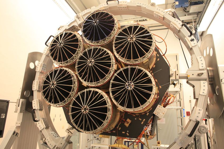
Abstract
Due to the high stellar density in globular clusters (GCs), they provide an ideal envi-
ronment for the formation of X-ray luminous objects, e.g. cataclysmic variables and
low-mass X-ray binaries. Those X-ray sources have, in the advent of ambitious observa-
tion campaigns like the eROSITA mission, become accessible for extensive population
studies.
During the course of this thesis, X-ray data in the direction of the Milky Way’s GCs
was extracted from the eRASS1 All-Sky Survey and then analyzed. The first few chap-
ters serve to provide an overview on the physical properties of GCs, the goals of the
eROSITA mission and the different types of X-ray sources. Afterwards, the methods
and results of the analysis will be presented.
Using data of the eRASS1 survey taken between December 13th, 2019 and June 11th,
2020, 113 X-ray sources were found in the field of view of 39 GCs, including Omega Cen-
tauri, 47 Tucanae and Liller 1. A Cross-correlation with optical/infrared catalogs and
the subsequent analysis of various diagrams enabled the identification of 6 foreground
stars, as well as numerous background candidates and stellar sources. Furthermore,
hardness ratio diagrams were used to select 16 bright sources, possibly of GC origin,
for a spectral analysis. By marking them in X-ray and optical images, it was concluded
that 6 of these sources represent the bright central emission of their host GC, while 10
are located outside of the GC center. For 3 out of 4 soft sources, the GC membership
was verified by plotting their counterparts in optical/infrared color-magnitude diagrams
of the host GC.
Contents
   List of Figures . . . . . . . . . . . . . . . . . . . . . . . . . . . . . . . . . . . . III
   List of Tables . . . . . . . . . . . . . . . . . . . . . . . . . . . . . . . . . . . . V

1 Introduction                                                                                                                         1

2 Globular Clusters                                                                                                                    2
  2.1 Formation, Age, Composition . . . . . . . . . . . . . . . . . . . . . . . .                                                      3
  2.2 Shape and Physical Properties . . . . . . . . . . . . . . . . . . . . . . . .                                                    4
  2.3 Color-Magnitude Diagrams . . . . . . . . . . . . . . . . . . . . . . . . . .                                                     5

3 eROSITA Mission and X-ray Sources                                                                                                     6
  3.1 eROSITA Mission . . . . . . . . .        .   .   .   .   .   .   .   .   .   .   .   .   .   .   .   .   .   .   .   .   .   .    6
  3.2 X-ray Sources . . . . . . . . . . .      .   .   .   .   .   .   .   .   .   .   .   .   .   .   .   .   .   .   .   .   .   .    7
      3.2.1 Foreground Sources . . . .         .   .   .   .   .   .   .   .   .   .   .   .   .   .   .   .   .   .   .   .   .   .    8
      3.2.2 Background Sources . . .           .   .   .   .   .   .   .   .   .   .   .   .   .   .   .   .   .   .   .   .   .   .    8
      3.2.3 Globular Cluster sources .         .   .   .   .   .   .   .   .   .   .   .   .   .   .   .   .   .   .   .   .   .   .    8

4 Analysis of eROSITA Data                                                                                                             11
  4.1 Source Selection . . . . . . . . . . . . . . . .                 .   .   .   .   .   .   .   .   .   .   .   .   .   .   .   .   11
  4.2 Hardness Ratios and Count Rates . . . . . .                      .   .   .   .   .   .   .   .   .   .   .   .   .   .   .   .   12
  4.3 Cross-matching with other catalogues . . . .                     .   .   .   .   .   .   .   .   .   .   .   .   .   .   .   .   13
  4.4 Interpreting Diagrams . . . . . . . . . . . .                    .   .   .   .   .   .   .   .   .   .   .   .   .   .   .   .   14
      4.4.1 Foreground and Background sources                          .   .   .   .   .   .   .   .   .   .   .   .   .   .   .   .   14
      4.4.2 Hardness Ratio Diagrams . . . . . .                        .   .   .   .   .   .   .   .   .   .   .   .   .   .   .   .   16
  4.5 Analysis of Globular Cluster Sources . . . .                     .   .   .   .   .   .   .   .   .   .   .   .   .   .   .   .   19

5 Conclusion                                                                                                                           38

6 Tables with Globular Cluster and Source Parameters                                                                                   40

Appendix                                                                                                                               47

Acknowledgements                                                                                                                       49

Bibliography                                                                                                                           51

Eigenständigkeitserklärung                                                                                                           56

                                                                                                                                        I
List of Figures
2.1 Optical image of the globular cluster Messier 80. . . . . . . . . . . . . . . 2
2.2 Distribution of the GCs in the Milky Way. . . . . . . . . . . . . . . . . . 3
3.1 The eROSITA X-ray telescope. . . . . . . . . . . . . . . . . . . . . . . . 6
4.1 Distance-magnitude diagram (Gaia g magnitude over distance). . . . . . 14
4.2 allWISE categorization of celestial objects. . . . . . . . . . . . . . . . . . 15
4.3 Infrared color-color diagram (allWISE bands W1-W2 over W2-W3). . . . 16
4.4 HR-HR diagram (HR2 over HR1 ). . . . . . . . . . . . . . . . . . . . . . . 17
4.5 HR-count rate diagram (C0 over HR1 ). . . . . . . . . . . . . . . . . . . . 18
4.6 HR-count rate diagram (C0 over HR2 ). . . . . . . . . . . . . . . . . . . . 18
4.7 Optical and X-ray images of Liller 1 . . . . . . . . . . . . . . . . . . . . . 22
4.8 Spectrum of Liller-1-86. . . . . . . . . . . . . . . . . . . . . . . . . . . . 22
4.9 Optical and X-ray images of Terzan 2 . . . . . . . . . . . . . . . . . . . . 23
4.10 Spectrum of Terzan-2-80. . . . . . . . . . . . . . . . . . . . . . . . . . . . 24
4.11 Spectrum of Terzan-2-81. . . . . . . . . . . . . . . . . . . . . . . . . . . . 24
4.12 Optical and X-ray images of NGC 1851 . . . . . . . . . . . . . . . . . . . 24
4.13 Spectrum of NGC-1851-13. . . . . . . . . . . . . . . . . . . . . . . . . . . 25
4.14 Optical and X-ray images of NGC 2808 . . . . . . . . . . . . . . . . . . . 25
4.15 Spectrum of NGC-2808-20. . . . . . . . . . . . . . . . . . . . . . . . . . . 26
4.16 Optical and X-ray images of NGC 5139 . . . . . . . . . . . . . . . . . . . 27
4.17 Spectrum of NGC-5139-45. . . . . . . . . . . . . . . . . . . . . . . . . . . 27
4.18 Optical and X-ray images of NGC 6441. . . . . . . . . . . . . . . . . . . 28
4.19 Spectrum of NGC-6441-101, source 1. . . . . . . . . . . . . . . . . . . . . 29
4.20 Optical and X-ray images of NGC 104 . . . . . . . . . . . . . . . . . . . 29
4.21 Spectrum of NGC-104-0. . . . . . . . . . . . . . . . . . . . . . . . . . . . 30
4.22 2mass near IR color-magnitude diagram (K over J-K) of NGC 104. . . . 31
4.23 Optical and X-ray images of NGC 6121 . . . . . . . . . . . . . . . . . . . 32
4.24 Spectrum of NGC-6121-64. . . . . . . . . . . . . . . . . . . . . . . . . . . 32
4.25 2mass near IR color-magnitude diagram (K over J-K) of NGC 6121. . . . 33
4.26 SkyMapper optical color-magnitude diagram (g over g-r) of NGC 6121. . 33
4.27 Optical and X-ray images of NGC 4372 . . . . . . . . . . . . . . . . . . . 34
4.28 Spectrum of NGC-4372-26. . . . . . . . . . . . . . . . . . . . . . . . . . . 35
4.29 Spectrum of NGC-4372-27. . . . . . . . . . . . . . . . . . . . . . . . . . . 35
4.30 2mass near IR color-magnitude diagram (K over J-K) of NGC 4372. . . . 36
4.31 SkyMapper optical color-magnitude diagram (g over g-r) of NGC 4372. . 36
6.1 Color-magnitude diagram (2mass band K over J-K). . . . . . . . . . . . . 47
IIIList of Figures
6.2 Color-magnitude diagram (SkyMapper band g over g-r). . . . . . . . . . 48
IVList of Tables
4.1 Globular Cluster ID with amount of eRASS1 sources in field of view. . . 12
4.2 X-ray bands of eRASS sources. . . . . . . . . . . . . . . . . . . . . . . . 12
4.3 Used catalogue bands and their wavelengths. . . . . . . . . . . . . . . . . 13
4.4 Globular cluster sources. . . . . . . . . . . . . . . . . . . . . . . . . . . . 19
4.5 Model parameters of analyzed sources. . . . . . . . . . . . . . . . . . . . 20
4.6 Overview of GC parameters. . . . . . . . . . . . . . . . . . . . . . . . . . 35
4.7 Probable nature of previously detected X-ray sources. . . . . . . . . . . . 37
6.1 Known GCs in the Milky Way. . . . . . . . . . . . . . . . . . . . . . . . 43
6.2 eRASS1 sources that were found via the source selection. . . . . . . . . . 46
V1 Introduction
The field of X-ray astronomy has experienced significant progress in the recent decades.
Modern X-ray satellites like Chandra and XMM-Newton have equipped us with im-
portant insights into the various X-ray source populations of the Universe, while the
ROSAT satelite delivered the first all-sky survey in the X-ray band. The most recent
addition to our inventory of X-ray instruments is the eROSITA telescope. Launched
into orbit in 2019, it aims to significantly improve our picture of the X-ray sky. After
completing 8 full scans of the celestial sphere, the eROSITA All-Sky survey will be
finished in 2023.
Among other sources, X-rays are emitted by hot intergalactic material, active galactic
nuclei (AGNs) and X-ray binaries.
X-ray binaries categorize X-ray emitting binary star systems, e.g. main-sequence stars
with a white dwarf (Cataclysmic Variables) or a neutron star companion (Low-mass X-
ray binaries), as well as systems of two main-sequence-stars (active binaries) and others.
Although X-ray binaries can occur in the Galactic disk, they are far more abundant in
the dense cores of GCs. The high stellar density leads to a high rate of stellar encounters
and thus drives the formation of these systems.
Studying observations of GCs is therefore a crucial branch of X-ray astronomy and,
following the launch of the Chandra telescope, enabled the identification of over 1500
X-ray sources (Pooley, 2010). The goal of this thesis is to improve our understanding of
these source populations by analyzing the X-ray sources detected in the first eROSITA
scan of the celestial sphere: eRASS1.
Since the field of view of the Milky Way’s GCs is typically obscured with foreground
stars and background galaxies/AGNs, it is important to identify these objects and
exclude them from further analysis. This can be achieved by cross-matching the X-
ray sources with catalogues at other wavelengths and investigating their counterparts.
Afterwards, the focus is laid upon the analysis of the GC sources. For detections
with sufficient count rates, physical properties can be constrained through a spectral
analysis. Furthermore, imaging software can be used to display the position of the
detected sources. Color-magnitude diagrams unveil whether a source coincides with a
stellar branch of the investigated GC.
During the course of this thesis, those methods will be used to acquire new information
about the X-ray sources detected in the eRASS1 scan. It turns out that some GC sources
represent the bright central emission of the GC, while others are located outside of the
central GC region. Further analysis is required to confidently constrain the nature of
these sources.
12 Globular Clusters
While the galactic disk of spiral galaxies is typically filled with a variety of objects and
matter, e.g. stars, gas and dust, the outer galactic regions remain relatively empty.
There is one kind of celestial bodies, however, that is almost exclusively found in the
galactic halo: globular clusters (GCs).
GCs are compact agglomerates of old, metal-poor stars, with a density increasing from
approximately 0.4 stars per cubic parsec in the outer regions to 100 - 1000 stars per
cubic parsec in the central core. In total, GCs typically contain a few hundred thousand
stars (Talpur, 1997). Due to their high density, GCs are strongly bound by gravity and
therefore possess a symmetrical, roughly spherical shape. This lies in contrast to the
asymmetrically arranged open star clusters, which are located in the galactic disk and
encompass up to a few thousand stars (Frommert et al., 2007). GCs can be interpreted
as an intermediate object between such open star clusters and more massive celestial
bodies, e.g. nuclear star clusters and dwarf galaxies, due to the fact that they show
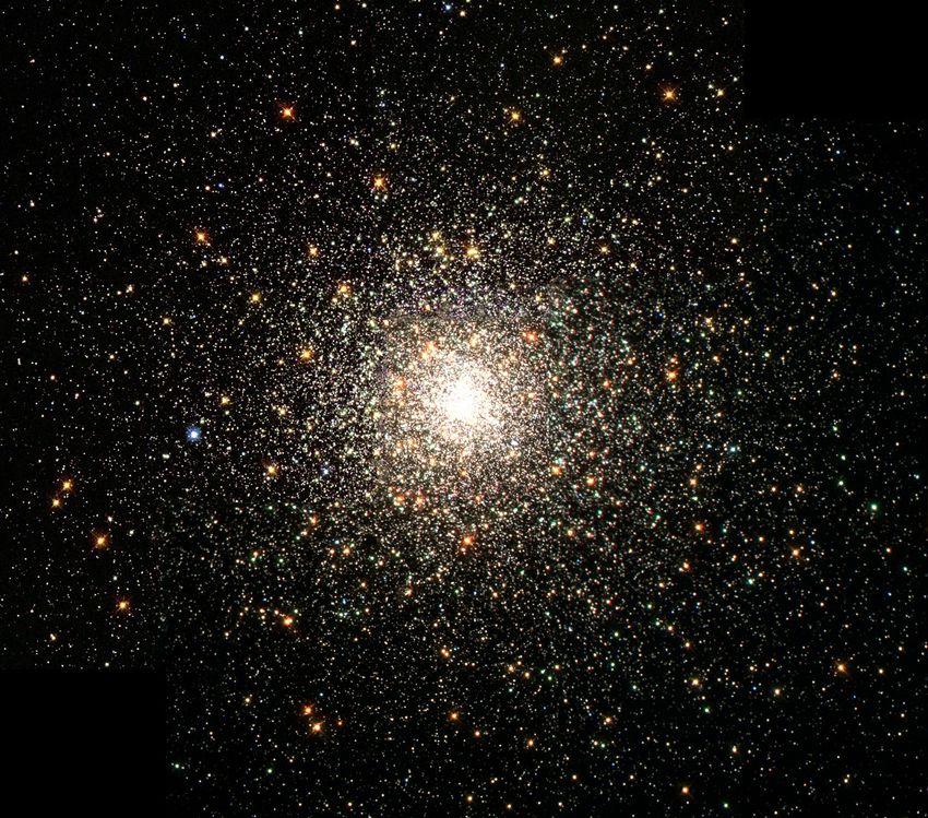
signs of chemical evolution (Gratton et al., 2019). An optical image of the globular
cluster Messier 80 is shown in Figure 2.1.
Fig. 2.1: Optical image of the globular cluster Messier 80 (Messier 80 2017).
Messier 80 is located in the Scorpius Constellation south to the center of the Milky
22 Globular Clusters
Way. It accounts for one of Milky Way’s most densly populated GCs (Carretta et al.,
2015).
In general, GCs are rather common, and can be found in the vicinity of nearly every
sufficiently massive galaxy (Harris, 1991). The Milky Way alone is orbited by at least
147 GCs (Harris, 1997). The precise number remains unknown, however, since some
Galactic regions cannot be properly observed due to obscuration by dust in the Galactic
disk. According to estimates, about ten to twenty local GCs are still undiscovered
(Ashman et al., 1992).
The GCs are positioned in a roughly spherical halo around the Milky Way. Many are
located close to the Galactic center, but fairly few are close to the Galactic plane. A
map of the GC distribution in the Milky Way is shown in Figure 2.2.
Fig. 2.2: Left: Spatial distribution of the inner GCs in the Milky Way in the YZ plane.
The Galactic center is positioned at (0,0). Right: Spatial distribution of the
more distant GCs. (Harris, 2001).
The largest galaxy in our cosmic neighborhood, the Andromeda Galaxy, may contain
up to 500 GCs (Barmby et al., 2001). Massive elliptical galaxies, such as M87, likely
account for as many as 13000 GCs (McLaughlin et al., 1994).
During the course of this section, the most important physical aspects of GCs will be
reviewed.
2.1 Formation, Age, Composition
For the largest part, the formation of GCs takes place in areas of efficient star formation
with exceptionally high densities, e.g. in interacting galaxies and starburst regions
(Elmegreen et al., 1999). However, GCs are among the oldest objects in a galaxy. Those
star formation processes presumably ended a long time ago and thereby exhausted the
amount of available gas and dust. In accordance to that, observations show that they
32 Globular Clusters are dust- and gas-free (Talpur, 1997). It is possible that GCs evolved from even larger collections of stars, known as super star clusters. Only very few of those objects have been discovered in the Milky Way, such as Westerlund 1 and NGC 3603 (ESO, 2005). One of the key goals of studying GCs is to determine their age and therefore improve our understanding of their formation process in respect to the host galaxy. This is of special interest, since GCs formed before the end of reionization (12.8 Gyrs ago at z ≈ 6) might have played a role in reionizing the Universe. It is also possible, however, that most GCs were shaped during the peak in the cosmic star formation rate at z ≈ 2. Observations of almost 70 GCs in the Milky Way point towards the coexistence of two separate GC populations: a dominant branch of old, mostly metal-poor GCs, and a younger, higher-metallicity branch. By deriving age-metallicity relations using color-magnitude diagrams from observations of the ACS on board of the Hubble Space Telescope, those GC populations have been estimated to be approximately 12.5 Gyrs and 11.5 Gyrs old. However, due to the large uncertainties of those results, formation during the same time period cannot be ruled out. Furthermore, it is possible that the younger branch GCs have been accreted from satellite galaxies like the Sagittarius Dwarf Spheroidal Galaxy (Forbes et al., 2018). In addition to the initial formation of the entire GCs, it is also important to consider the individual stars. To this day, it remains unclear whether the stars in a GC are generated during a single event, or across multiple formation periods over hundreds of millions of years. While the better part of stars in most GCs is at roughly the same stage of stellar evolution, some GCs feature distinct star populations. Close approaches of large molecular clouds can significantly alter their star formation history. Such events likely triggered a second round of star formation in the GCs of the Large Magellanic Cloud during their early ages (Piotto, 2009). It is also possible to attribute this kind of multiplicity to mergers of distinct GCs, especially in dense regions (Amaro-Seoane et al., 2013). Despite possible variations in the star formation history, GCs typically exhibit old and metal-poor stars. They can be compared to stars located in the bulge of spiral galaxies. However, they are confined inside a much smaller volume (Talpur, 1997). The enormously high mass of GCs like Omega Centauri and Mayall II indicates, that some GCs embody the cores of previously consumed dwarf galaxies (Bekki et al., 2003). According to estimates, this holds true for roughly one fourth of the Milky Way’s GC population (Forbes et al., 2010). 2.2 Shape and Physical Properties While the GCs in the halo of the Milky Way and the Andromeda Galaxy are mostly spherical, those in the Small and Large Magellanic Cloud posses a more elliptical shape. Such ellipticities can result due to tidal interactions between the stars in a GC (Frenk et al., 1980). Following their formation, the stars exert a gravitational force on each other, and thereby continuously alter their motion through the GC. After the so-called relaxation time, their velocity has been completely renewed. In general, GCs remain gravitationally bound as long as most of the stars haven’t exceeded their life span 4
2 Globular Clusters

(Benacquista, 2006).
Due to the high amount of stars concentrated in a small volume, GCs are extremely lu-
minous. Within the Local Group, the GC luminosities can be represented by a gaussian
curve. This luminosity distribution is called the Globular Cluster Luminosity Function
and it yields an average magnitude MV and a variance σ 2 . For GCs in the Milky Way,
those values correspond to MV = −7.20 ± 0.13 and σ 2 = 1.1 ± 0.1 (Secker, 1992).
In the Milky Way, NGC-5139, also referred to as Omega Centauri, represents the
brightest GC. At a distance of 5.1 kpc from the Sun, its absolute visual magnitude
of −10.24 mag appears as bright as 3.68 mag (Harris, 1997). Typically, small GCs pos-
sess masses on the order of 104 M , while the largest ones exceed 106 M . Omega
Centauri, for instance, has a mass of (3.55 ± 0.03) · 106 M (Baumgardt et al., 2018).
The corresponding radii can be calculated in different ways. Since the luminosity of GCs
decreases, along with the star-density, with distance from the core, one can define a core-
radius Rc , aswell as a half-light radius Rh . While the core-radius marks the distance,
at which the apparent luminosity of the GC surface has decreased to 50 percent of the
central value (Janes, 2000), the half-light radius contains the area that emits half of
the total luminosity. Most GCs possess a half-light radius lower than 10 pc. However,
a small fraction has exceptionally high radii, as in case of Palomar 14, which has a
half-light radius of 25 pc (Bergh et al., 2007). Additionally, the half-mass radius Rm ,
and the tidal radius Rt are introduced (Buonanno et al., 1994). The half-mass radius
encompasses half of the GC’s mass and can be used to determine whether the GC has
an unusually dense core. The tidal radius on the other hand, marks the distance from
the core, at which the gravitational pull of the host galaxy becomes strong enough to
separate the stars from the GC (Janes, 2000).

2.3 Color-Magnitude Diagrams
A Color-Magnitude Diagram (also called Hertzsprung-Russell diagram) represents the
correlation between the absolute magnitude and the color index of a selection of stars.
The color index B −V of a star can be calculated by subtracting the star’s magnitude in
the V-band from its magnitude in the B-band. Since the stars of a GC typically formed
in the same time period from the same materials, plotting the absolute magnitude
of these stars over their color index will often yield a well-defined curve. The only
dissimilarity between those stars is their initial mass. This lies in contrast to galactic
star populations, where this sloping curve, the main-sequence, represents stars of diverse
compositions, ages and masses (Sandage, 1957).

                                                                                         5
3 eROSITA Mission and X-ray Sources
3.1 eROSITA Mission
eROSITA (extended ROentgen Survey with an Imaging Telescope Array) is an X-ray
instrument developed by the Max Planck Institute for extraterrestrial Physics (MPE).
On July 13, 2019, it has been launched from the Baikonour cosmodrome as a part of the
Russian-German Spectrum-Roentgen-Gamma (SRG) mission. The eROSITA mission
started on December 13, 2019 and aims to complete an all-sky survey in energy bands
between 0.2 and 8 keV by the end of 2023. An image of the eROSITA telescope is
displayed in Figure 3.1.
Fig. 3.1: The eROSITA X-ray telescope (Friedrich, 2019).
Alongside eROSITA, which is the primary X-ray telescope, the SRG observatory also
carries the ART-XC (Astronomical Roentgen Telescope X-ray Concentrator). The
ART-XC is an X-ray mirror telescope and complements the sensitivity of eROSITA
at higher energies. It was developed under the lead of the Russian Space Research In-
stitute IKI. Both instruments are attached to the Navigator spacecraft platform. Since
63 eROSITA Mission and X-ray Sources
the eROSITA mission was developed under german-russian collaboration, it has been
agreed to divide the observational data between the two nations. The southern hemi-
sphere has been assigned for studies by the german side, and the nothern hemisphere
for studies by the russian side.
The concept of the eROSITA instrument is an advancement of previously developed
devices by the MPE, e.g. the X-ray telescope for the ROSAT X-ray satelite mission.
The first complete all-sky survey with an imaging X-ray telescope was carried out by
ROSAT in energy bands between 0.1 and 2.4 keV. By completing 8 complete scans of
the celestial sphere, the eROSITA mission aims to increase the sensitivity of the ROSAT
All-Sky Survey by a factor of 25 and to provide the first imaging survey in the hard 2.3
- 8 keV band. Each of these eRASS scans will last 6 months.
The primary goal of the eROSITA mission is to detect large samples of galaxy clusters
up to redshifts z > 1. Such detections will greatly increase our understanding of the
large-scale structure of the universe and provide crucial new data for the testing of
cosmological models (Predehl et al., 2020). In particular, the results may constrain
the rate of expansion of the Universe and deliver new insights into the nature of Dark
Energy.
Galaxy Clusters can be detected due to X-ray emission from their hot intergalactic
material. The eROSITA mission is expected to find 50 - 100 thousand of such galaxy
clusters. Furthermore, it will enable the detection of obscured accreting black holes
in nearby galaxies and millions of distant active galactic nuclei (AGNs) (eROSITA
2021). Those new detections will provide important new insights into the evolution of
supermassive black holes (Predehl et al., 2020).
However, in addition to driving the study of cosmic structure evolution, the eROSITA
mission will also greatly impact the study of Galactic X-ray source populations, such as
supernova remnants, X-ray binaries, and active stars. The increased sensitivity of the
eROSITA all-sky survey will allow the identification of these objects and deliver new
insights into their properties.
Due to the high stellar density in GCs, they provide an ideal environment for the
formation of such X-ray luminous objects. Their population of luminous low-mass X-
ray binaries per unit stellar mass, for instance, is by a factor 100 higher than in the rest
of the Galaxy (Homer et al., 2002). A promising method of identifying and studying
X-ray luminous sources is therefore to target GC observations.
3.2 X-ray Sources
Within the framework of this study, the focus has been laid upon GC observations of
the eRASS1 scan of the celestial sphere. The source selection has yielded 113 detections
in the field of view of the Milky Way’s GCs. It is important to note, that those findings
only include sources within the southern hemisphere, which was assigned for german
studies. Those detections include foreground- and background sources, as well as X-
ray sources within the core and the outer regions of the GCs. The most commonly
detected X-ray sources in GCs are active binaries (ABs), cataclysmic variables (CVs),
millisecond Pulsars (MSPs) and low-mass X-ray binaries (LMXBs).
73 eROSITA Mission and X-ray Sources The goal of is this study is to identify the fore- and background sources within the 113 detections, and focus on the analysis of the GC sources (see chapter 4). The following sections serve to provide an overview over the different types of X-ray sources. 3.2.1 Foreground Sources Foreground sources are objects that are located in the field of view of an observation, but are positioned in the foreground of the observed source. They do not belong to the GCs and are typically stars within the spiral arms of the Milky Way. Therefore they are not interesting for this study and will be eliminated from further analysis. One way to identify foreground stars is by comparing their emission in different energy bands. Within the soft X-ray bands, their emission is typically much stronger than in harder X-ray bands. An example of this can be seen in Figure 4.18, where an X-ray emitting source is located to the right side of the GC extraction region. The soft nature of the emission indicates that the source is a foreground star. In addition, foreground sources can be identified through bright emission in optical and infrared bands. The flux of their optical counterpart exceeds the flux of their X-ray emission (Egg, 2020). 3.2.2 Background Sources Background sources are bright X-ray emitters that are located in the background of an observed source. This source category includes galaxies and AGNs. Although they are very distant, they still contribute to the X-ray flux. Since they don’t belong to the GCs, they will also be eliminated from further analysis. Background sources can be identified by analyzing their infrared counterparts. Radio counterparts, for instance, indicate that the source might be an AGN (Egg, 2020). 3.2.3 Globular Cluster sources Over the last couple of decades, ambitious observation campaigns have yielded im- portant new insights into the X-ray source populations of GCs. Einstein and ROSAT observations revealed an overabundance of low-luminosity X-ray sources (< 1033 erg s−1 ) compared to the Galactic field, while Uhuru and OSO-7 confirmed an enrichment with highly luminous X-ray sources (> 1036 erg s−1 ). Prior to the development of modern X-ray telescopes, the classification of those low-luminosity sources proved to be a big challenge. However, with the emergence of new instruments, e.g. the Chandra X-ray observatory, high-resolution observations enabled counterpart identifications and deliv- ered new constraints regarding the nature of those sources (through multiwavelength analysis). By now, Chandra observations revealed at least 1500 X-ray sources in over 80 GCs. Various studies confirmed a correlation between the number of detected X-ray sources and the stellar encounter rate of a GC (Pooley, 2010). Due to the high stellar densities in their cores, GCs often have extremely high stellar encounter rates (Bhattacharya et al., 2017) (including most of the GCs observed with 8
3 eROSITA Mission and X-ray Sources

Chandra (Bassa et al., 2004)). Such conditions provide an ideal environment for the for-
mation of various binary systems (Homer et al., 2002), including LMXBs in quiescence,
CVs, ABs and MSPs. High-luminosity LMXBs were found to be orders of magnitude
more common per unit mass compared to the rest of the Galaxy (Pooley, 2010). Most
of these systems were formed via close stellar encounters (Bassa et al., 2004). The
majority of X-ray binaries is expected to be positioned within the GCs half-mass radius
(Servillat et al., 2008).

Low-mass X-ray Binaries

The brightest X-ray sources in GCs are low-mass X-ray binaries (Bassa et al., 2004).
They are binary star systems composed of a donor and a neutron star or black hole
accretor. The donor is either a main sequence star, a red giant or a white dwarf.
The accretor is surrounded by an accretion disk due to mass transfer from the donor.
The infalling matter leads to a release of gravitational potential energy in the form of
X-rays. Hence, LMXBs are typically bright in X-rays, but faint in the optical. The
accretion disk is the brightest part of the system (Tauris et al., 2006). In addition,
some neutron star LMXBs have been observed to emit periodic X-ray bursts, which
are typically by a factor 100 more luminous than their ordinary emission. Such events
are categorized in Type I and Type II X-ray bursts. They are believed to occur when
the accumulated matter from the donor star leads to bursting fusion reactions on the
neutron star’s surface. Type I bursts are a consequence of thermonuclear runaway and
gradually decline after a sharp rise in luminosity. Type II bursts, on the other hand,
result from gravitational potential energy release and can occur many times in a row as
a quick pulse shape. Type I bursts are far more common. In fact, Type II bursts have
only been detected from two sources (Lewin et al., 1993), e.g. the Rapid Burster in the
GC Liller 1 (see section 4.5).
Despite the fact that GCs only contribute to ∼ 0.01 % of the total stellar mass within
the Galaxy, 13 out of the ∼ 100 Galactic LMXBs are hosted by GCs (Zurek et al.,
2009), most of them in quiescence (Pooley, 2010).
This can be explained by the fact that some dynamical LMXB formation channels might
only exist in the dense cores of GCs. LMXBs can be created by exchange interactions
between neutron stars and primordial binaries, the tidal capture of a main sequence
star by a neutron star, or by direct collision of a neutron star with a red giant (Zurek
et al., 2009). The evolution of a LMXB out of a primordial binary system on the other
hand, is far less likely (Servillat et al., 2008).
It is possible that a large fraction of bright LMXBs in GCs are ultracompact X-ray
binaries (UCXBs). UCXBs categorize interacting binaries that have very small binary
seperations a ' 1010 cm and orbital periods P . 1 hr. In the Galactic field, UCXBs
only account for a small percentage of LMXBs (Zurek et al., 2009).
A subcategory of LMXB are the so-called Millisecond Pulsars (MSPs). They are pulsars
with short rotational periods, and about as luminous as CVs (Bassa et al., 2004). MSPs
are believed to be neutron stars from LMXB systems, that have been spinned up due
to angular momentum transfer from the companion star. Such MSPs are typically
observed in the radio band and can therefore by identified by their radio counterpart

                                                                                      9
3 eROSITA Mission and X-ray Sources (Servillat et al., 2008). In some cases, however, a portion of the MSP surface near the magnetic poles can generate X-ray radiation due to heating by relativistic particles from the magnetosphere. In addition, it is possible that those relativistic particles generate non-thermal, pulsed X-ray emission (Bhattacharya et al., 2017). High-metallicity GCs with high stellar encounter rates typically exhibit a larger abundance of MSPs (Saracino et al., 2015). Cataclysmic Variables In terms of brightness, LMXBs are followed by white dwarfs that are accreting material from low-mass companions (CVs). Such systems are common within the Galactic field, and even more abundant in GCs. They can either originate from primordial binaries, or result from close stellar encounters. However, a correlation between the number of faint sources and the stellar encounter rate of a GC indicates that most GC CVs are formed via close stellar encounters (Bassa et al., 2004). They can be identified by a blue, variable optical counterpart (Servillat et al., 2008). Active Binaries Chromospherically or magnetically active binaries are typically fainter than LMXBs and CVs. They are categorized in 3 different types. The first two are detached binary sys- tems of either two main sequence stars, or a main sequence star and a giant/sub-giant, while the third type are contact binaries (Bassa et al., 2004). ABs can be identified by their main-sequence-like, variable optical counterparts (Servillat et al., 2008). 10
4 Analysis of eROSITA Data

4.1 Source Selection

The observational data of the GCs in the vicinity of the Milky Way has been acquired
from The catalogueue of Globular Clusters (Harris, 1997). The catalogue provides a
database of parameters on the mentioned GCs, including measurements for the cluster
distance, luminosity, spectral types, metallicity, as well as other structural and dynam-
ical parameters. In addition to the list of parameters, the catalogueue also provides
a complete bibliography for the literature sources of every displayed quantity. The
parameters are frequently updated, as new data emerges.
The goal of this section is to extract positional and dimensional data of the GCs, that
are listed in the catalogue, in order to identify eRASS1 sources in the field of view of
those GCs for further analysis. This was achieved by downloading an ascii-table of
all 147 GCs from the VizieR website. A complete table of the 147 GCs (Table 6.1),
including their IDs, as well as their position (RA = right ascension, DE = declination),
their distance (Rsun = distance to the sun, Rgc = distance to the Galactic center) and
their radii (Rc = core radius, Rm = half-mass radius) is displayed in chapter 6.
In order to select all of the important sources encompassed by the GCs, the area for
source-selection has been defined as a circle with a radius of 5 · Rm around the center
of the considered GC. Those regions were used to acquire fits-files containing data of
the eRASS1 sources in field of view of all 147 GCs. It is important to note, though,
that the available eRASS data only includes half of the sky (the other half is reserved
for russian studies). The results of the source-selection yielded 113 detections, with 39
of the 147 GCs containing at least one eRASS1 source. All GCs with at least three
eRASS1 sources in their field of view are listed in Table 4.1.
The acquired data includes the eRASS catalogue ID of the sources, as well as their
position (RA and DE (J2000)), spatial expansion, the amount of detected X-ray counts
and the count rate. The latter two are separated into three distinct energy bands, and an
additional band encompassing the total number of counts. The corresponding energy
ranges are displayed in Table 4.2. Those energy bands will be used to calculate the
hardness ratios of the eRASS sources in the next section. The X-ray counts for each
source were detected in a circle with a radius of 42 arcsec around the source position.
The coordinates, counts and count rates of all 113 detections are listed in Table 6.2.
Source 112 has been discarded from further analysis due to missing data.

                                                                                      11
4 Analysis of eROSITA Data
ID Sources
NGC 5139 16
NGC 4372 11
NGC 104 9
NGC 6397 8
NGC 5053 5
NGC 6121 5 X-ray band Energy range
NGC 1851 4 total 0.2 − 5.0 keV
NGC 2808 4 soft 0.2 − 0.6 keV
NGC 6101 4 medium 0.6 − 2.3 keV
NGC 6441 3 hard 2.3 − 5.0 keV
NGC 6752 3
NGC 362 3 Tab. 4.2: X-ray bands of eRASS sources.
Terzan 2 3
Liller 1 3
Tab. 4.1: Globular Cluster ID with
amount of eRASS1 sources in
field of view.
4.2 Hardness Ratios and Count Rates
The eRASS source catalogue provides the X-ray counts, as well as the X-ray count rate
of the sources for each energy band. Those values can be used to calculate the hardness
ratios HRi :
Bi+1 − Bi
HRi = (4.1)
Bi+1 + Bi
where Bi are the total counts in the corresponding X-ray band for i ∈ {1, 2, 3}. Those
calculations have been performed in accordance with Sasaki et al., 2018, using the
counts instead of the count rates, as they provide more reliable results in the considered
case.
By analyzing hardness ratios, one can acquire new information about the spectral prop-
erties of the investigated sources. They are particularly useful for the comparison of
emission characteristics in different parts of the electromagnetic spectrum, since one
hardness ratio contains information on two distinct bands. In the considered case, HR1
represents a relation between the soft (i = 1) and the medium (i = 2) band, and HR1
a relation between the medium and the hard (i = 3) band. The corresponding errors
∆HRi are defined as (Sasaki et al., 2018):
p
(Bi+1 ∆Bi )2 + (Bi ∆Bi+1 )2
∆HRi = 2 (4.2)
(Bi+1 + Bi )2
In the following, the count rates of a specific energy band are denoted as Ci , and the
corresponding errors as ∆Ci . Since count rate errors are not given by the eRASS source
124 Analysis of eROSITA Data
catalogue, they must be calculated using the relation
Bi
τi = (4.3)
Ci
where τi represents the exposure time of the observation. Subsequently, the count rate
error can be written as:
∆Bi
∆Ci = (4.4)
τi
The hardness ratios HR1 and HR2 have been calculated for each selected eRASS source
with a self-written python 3 script. During the course of this thesis, the hardness ratios,
as well as the count rates, will be used to acquire new information regarding the nature
of the sources.
4.3 Cross-matching with other catalogues
The investigation of fluxes throughout the whole electromagnetic spectrum represents,
similarly to the comparison of distinct X-ray bands, a viable method to acquire new
knowledge on the analyzed sources. This is due to the fact that many types of celestial
objects display characteristic emission features, which provide hints on their chemical
makeup, as well as their origin. Henceforth, the goal of this section will be to cross-match
the selected eRASS sources with surveys that were carried out at other wavelengths,
and thereby acquire the fluxes of their counterparts. Afterwards, the new data can be
used to provide new constraints on the type of object represented by the source.
catalogue Band Wavelength [µm]
allWISE W1 3.4
allWISE W2 4.6
allWISE W3 12
allWISE W4 22
2mass J 1.25
2mass K 2.17
SkyMapper g 0.40 - 0.67
SkyMapper r 0.48 - 0.73
gaia g 0.3 - 1.1
Tab. 4.3: Used catalogue bands and their wavelengths (Cutri et al., 2012, About 2MASS
2006, Data Release DR2. Release documentation 2019, Gaia DR2 Passbands
2018).
Within the framework of this thesis, a script designated as artemis (written by Jonathan
Knies, Dr. Karl Remeis-Observatory Bamberg), which operates upon the NWAY al-
gorithm, will be used for the cross-matching with other catalogues. Those catalogues
are based on observational data from the Wide-field Infrared Survey Explorer mission
(allWISE ), the Two Micron All Sky Survey (2mass), the SkyMapper telescope, as well
134 Analysis of eROSITA Data
as the Gaia space observatory. 2mass provides counterparts in the near-infrared band,
whereas the SkyMapper and Gaia catalogue provide optical counterparts. In addition,
the Gaia catalogue also provides distance measurements.
The electromagnetic bands displayed in Table 4.3 are of particular interest for the
following analysis and classification of the eRASS sources selected in section 4.1.
4.4 Interpreting Diagrams
To identify and study the X-ray sources located in the GCs of the Milky Way, other
sources, e.g. foreground stars and background sources have to be eliminated. This
was carried out by using the flux data, as well as the obtained counterparts, for the
modelling of a variety of different plots. The subsequent classification was performed
with an analysis of the source distribution in the resulting diagrams: discrimination of
the sources in accordance to specific criteria.
4.4.1 Foreground and Background sources
As the Gaia space observatory was designed for astrometry (ESA, 2013), it acommo-
dates for valuable distance measurements, that can be used for the identification of
sources located outside of the proximity of the investigated GCs.
8 Rup-106-37
Stellar sources
Count Rate < 0.5
10 Background candidates
NGC-5053-41
NGC-5053-42 Foreground sources
12
NGC-6121-67
14 NGC-6723-107
NGC-6121-65 NGC-6121-66
g
16 NGC-4372-34
NGC-4372-32
18 NGC-5053-43
NGC-4372-36
20 NGC-5053-40
NGC-5053-44 NGC-5897-61
NGC-6101-71 NGC-6101-69NGC-6101-72
NGC-5897-62 NGC-6121-68
0 1000 2000 3000 4000 5000 6000 7000
distance in pc
Fig. 4.1: Distance-magnitude diagram (Gaia g magnitude over distance).
144 Analysis of eROSITA Data
The sources, for which the cross-match with the gaia catalogue was successful, have been
assigned to the GC in their field of view and implemented in the distance-magnitude
diagram shown in Figure 4.1. Out of the 18 sources that were matched to a source from
the gaia catalogue, 16 yielded a considerably smaller distance measurement, than the
corresponding GC. Despite that, the parallax distance measurements were accompanied
by large uncertainties for all but six of the 18 sources. The significance of those mea-
surements has been checked by examining whether they fulfil the four relevant criteria
established by Arenou et al., 2018 and Lindegren et al., 2018.
However, due to the lack of flux data for the gaia GBP and GRP band, the examination
did not yield meaningful results.
In conclusion, the six sources with low distance uncertainties (marked by blue crosses,
seen in the upper left corner of Figure 4.1) were classified as foreground stars, whereas
the remaining sources were ignored.
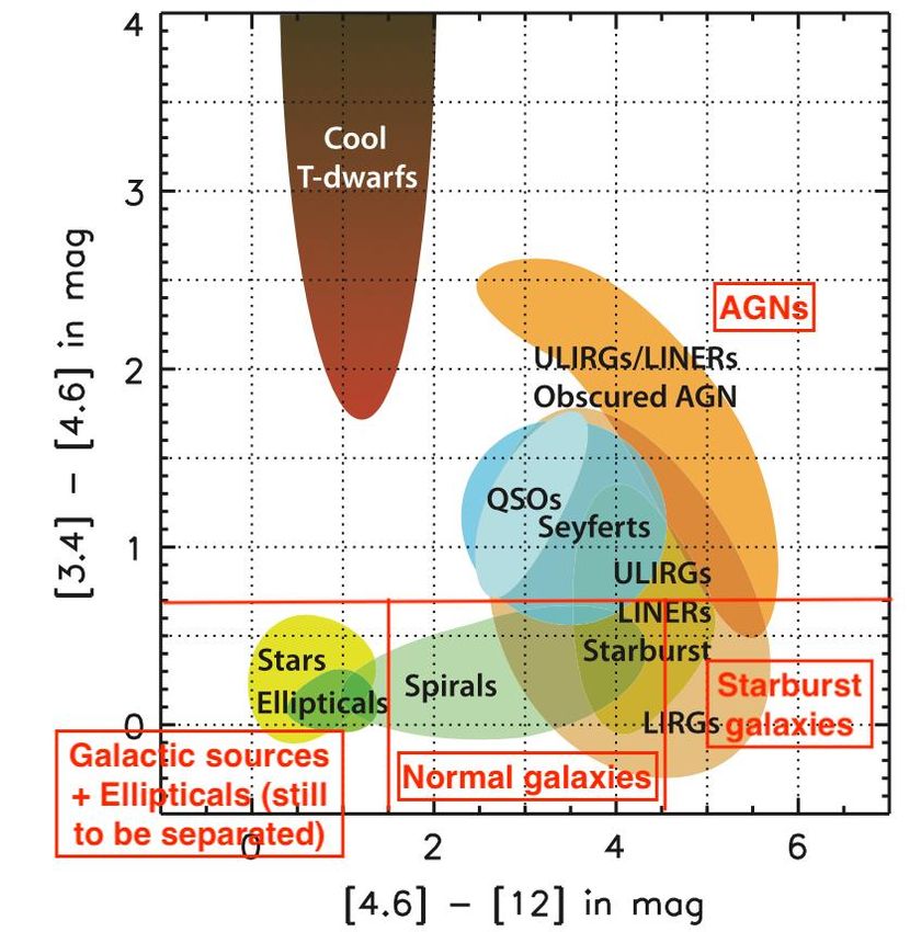
Fig. 4.2: Categorization of celestial objects according to their position in the allWISE
infrared color-color diagram (W1-W2 over W2-W3) (Wright et al., 2010), red
descriptions were added by Manami Sasaki.
In the next step of source identification, the eRASS sources were classified according to
the categorization scheme displayed in Figure 4.2. Here, celestial bodies are separated
into AGNs, Galactic sources and different kinds of galaxies according to their positioning
154 Analysis of eROSITA Data
in an infrared color-color diagram, where the allWISE bands W1-W2 are plotted over
the bands W2-W3.
The same diagram including the cross-matched allWISE magnitudes of the eRASS
sources is shown in Figure 4.3. As apparent from Figure 4.2, Galactic sources and
elliptical galaxies are found in the lower-left section with W2 − W3 < 1.5 and W1 −
W2 < 0.7. Therefore, all sources, which fulfil these criteria, have been classified as
stellar soruces (marked as light-blue stars).
AGNs on the other hand, are located in the section with W1 − W2 > 0.7, and starburst
galaxies in the section with W2 − W3 > 4.5 and W1 − W2 < 0.7. In accordance to
that, the corresponding eRASS sources have been classified as background candidates
(marked as red crosses). The normal galaxies section can also include globular cluster
sources.
1.5 Central GC object
Stellar sources
1.0 Count Rate < 0.5
GC sources
Background candidates NGC-5139-45
0.5 Foreground sources
NGC-4372-26
0.0 NGC-6121-64
NGC-4372-27
Terzan-2-81
W1 - W2
Terzan-2-80
NGC-1851-14
0.5 NGC-2808-20
NGC-1851-13
1.0
1.5 NGC-104-0
2.0
2 1 0 1 2 3 4
W2 - W3
Fig. 4.3: Infrared color-color diagram (allWISE bands W1-W2 over W2-W3).
4.4.2 Hardness Ratio Diagrams
Further constraints on the nature of the sources have been acquired by plotting their
hardness ratios and count rates. Since the X-ray counts are split into three distinct
energy bands, only two sets of hardness ratios can be obtained: HR1 and HR2 (see
section 4.2). These are plotted against each other in a HR1 -HR2 diagram shown in
Figure 4.4.
In addition, the plot contains six lines based on PyXspec spectral analysis models
created by Sara Saeedi. Those lines represent regions of expected hardness ratio values
164 Analysis of eROSITA Data
in dependence of the physical properties of the sources. The models include three
power-law models (photon-index = 1, 2, 3) and three plasma temperature models (kT
= 0.2 keV, 1.0 keV, 2.0 keV) at column densities between NH = 0.01 · 1022 cm−2 and
NH = 100 · 1022 cm−2 . However, the distribution of the sources does not show a clear
correlation to the models. This leads to the conclusion, that the standard eROSITA
energy bands are not useful for source-classification. In future studies, this could be
dealt with by adding an additional energy band for the X-ray counts.
1.00
0.75
0.50 N_H = 0.5
N_H = 0.1
0.25 N_H = 0.01
N_H = 0.5
kT = 0.2
0.00
HR2
kT = 1.0
kT = 2.0 N_H = 0.1 nH = 0.5
0.25 Photon-index 1
Photon-index 2
N_H = 0.01
N_H = 0.5
nH = 0.1
Photon-index 3 N_H = 0.01
0.50 Central GC object
Stellar sources N_H = 0.1
N_H = 0.01
Count Rate < 0.5 N_H = 0.5
0.75 GC sources
N_H = 0.01 N_H = 0.1
Background candidates
Foreground sources N_H = 0.01
1.00 N_H = 0.1 N_H = 0.5
1.00 0.75 0.50 0.25 0.00 0.25 0.50 0.75 1.00
HR1
Fig. 4.4: HR-HR diagram (HR2 over HR1 ) with power-law and plasma temperature
models. NH values are given in 1022 cm−2 .
The figures in this section have been created under the assumption that all sources
have a sufficiently high number of counts for the calculation of hardness ratios. This
is not the case, however, as indicated by the sources on the bottom and right-hand
edge of Figure 4.4. In order to provide a clear overview on the X-ray luminosity of
the sources, the total count rate C0 has been plotted against HR1 and HR2 , as can
be seen in Figure 4.5 and Figure 4.6, respectively. Subsequently, all sources with a
total count rate C0 < 0.5 s−1 have been highlighted as light-green rhombuses. Although
some of them are likely GC sources, their X-ray intensity is not sufficient for confident
constraints on their properties. Therefore, those sources will not be further analyzed.
After subtraction of the fore- and background sources, as well as the sources with
insufficient X-ray counts, nine objects remained. It can be concluded, that those sources
are either part of a GC or represent a central GC object. Therefore, they have been
classified as GC sources and marked by orange crosses/rhombuses in all diagrams.
174 Analysis of eROSITA Data
102
Central GC object
NGC-1851-13 NGC-6441-101
Stellar sources
NGC-2808-20
Terzan-2-80
Count Rate < 0.5 Liller-1-86
101 GC sources
Background candidates Terzan-2-82
Total count rate
Liller-1-87
Foreground sources Liller-1-88
NGC-1851-16
NGC-6121-64 NGC-1851-14
NGC-104-0
100 NGC-4372-27 NGC-5139-45
NGC-4372-26
Terzan-2-81
10 1
0.75 0.50 0.25 0.00 0.25 0.50 0.75 1.00
HR1
Fig. 4.5: HR-count rate diagram (C0 over HR1 ).
103
Central GC object
Stellar sources
Count Rate < 0.5
102 NGC-1851-13 NGC-6441-101
GC sources
NGC-2808-20
Terzan-2-80 Background candidates
Foreground sources
Total count rate
Liller-1-86
101 Terzan-2-82 Liller-1-87
Liller-1-88
NGC-1851-16
NGC-6121-64 NGC-1851-14
100 NGC-104-0 NGC-5139-45
NGC-4372-27 NGC-4372-26 Terzan-2-81
10 1
1.0 0.8 0.6 0.4 0.2 0.0 0.2
HR2
Fig. 4.6: HR-count rate diagram (C0 over HR2 ).
184 Analysis of eROSITA Data
As apparent from Figure 4.5, the GC sources are clustered in the upper right corner
of the HR1 -count rate diagram. In addition to the nine initially classified GC sources,
seven stellar sources were located in the same region. Those have also been categorized
as GC sources.
Afterwards, each of these sources has been assigned to their host GC and flagged with a
corresponding designation. The designations have been constructed from the ID of the
GC and the source. All globular cluster sources, as well as their positional data, is listed
in Table 4.4. After a more detailed source-analysis in section 4.5, the presumed detection
type and the contained objects have also been added to the sources in Table 4.4.
GC ID NGC ID Src. RA [◦ ] DE [◦ ] Type Contains
Liller 1 86 263.351048 -33.387020 1 LMXB
Liller 1 87 263.367080 -33.398725 2
Liller 1 88 263.317705 -33.369826 2
Terzan 2 80 261.886976 -30.800186 1 LMXB
Terzan 2 81 261.828809 -30.828867 2
Terzan 2 82 261.904339 -30.789197 2
Caldwell 73 NGC 1851 13 78.525579 -40.043858 1 LMXB & MSP
Caldwell 73 NGC 1851 14 78.511218 -40.061486 2
Caldwell 73 NGC 1851 16 78.581367 -40.043111 2
Melotte 95 NGC 2808 20 138.009602 -64.866835 1 LMXB & CVs
Omega Cen NGC 5139 45 202.170112 -47.463716 2
NGC 6441 NGC 6441 101 267.550853 -37.050205 1 LMXB & MSPs
47 Tucanae NGC 104 0 6.010449 -72.081343 1 LMXB & others
Messier 4 NGC 6121 64 245.845533 -26.370861 2
Caldwell 108 NGC 4372 26 186.299651 -72.450269 2
Caldwell 108 NGC 4372 27 186.392734 -72.462313 2
Tab. 4.4: Globular cluster sources. Type 1: central GC region, Type 2: outside of GC
center.
4.5 Analysis of Globular Cluster Sources
Following the classification of the detected sources, the GC sources displayed in Table 4.4
have been further analyzed.
During the first step, optical images of the GCs have been acquired from the SkyView
website (SkyView, 2021). Since the GC sources are located in the southern hemisphere,
the DSS total band of the Optical:DSS survey has been chosen. Those images have
then been used to plot the positions of the eRASS1 sources (small green circles with
the corresponding source ID) and the source extraction region of each GC (large green
circle). This was achieved through a self-written shell script operating upon the image
tool SAOImageDS9. The results show the extent of the GC (five half-mass radii), as
well as the position/distance of the sources in respect to the GC core. In addition, it
can be seen whether the X-ray sources coincide with noticeably bright emission in the
optical band. The images are presented during the course of this section.
194 Analysis of eROSITA Data
Afterwards, the focus was laid onto the X-ray band. Using observational data from
the eRASS1 mission (acquired by Sara Saeedi), RGB X-ray images were created in a
similar way to the optical images. These images provide a more detailed insight into the
distribution of X-ray emission within the GCs and the X-ray emission characteristics of
the eRASS1 sources. Blue marks represent emission in the soft X-ray band, red marks
emission in the medium X-ray band, and green marks emission in the hard X-ray band
(see Table 4.2).
The images have been used to constrain the nature of the GC sources. For detections
in the central region of a GC, it can be concluded that they represent the emission of
sources within the GC core. Since the cores of GCs contain a large amount of sources
(on the order of 105 − 106 sources), often including X-ray emitters like CVs, MSPs,
ABs and LMXBs, it is possible that the detection is composed of the emission of a
large number of sources. Detections of this type have been classified as Type 1, while
detections outside of the central GC region have been classified as Type 2. Type 2
detections, which coincide with a peak in X-ray emission in the corresponding X-ray
image, presumably represent a single bright X-ray source or a small number of X-ray
emitting sources in close proximity to each other. However, some of the detections
generated relatively high X-ray counts although they don’t coincide with a peak in
emission in the X-ray images. These detections are mostly located close to the GC
center where the stellar density (and the amount of X-ray binaries) is still relatively
high. It is therefore possible that those detections were triggered by an above-average
number of bright X-ray emitters in the detection circle (with a radius of 42 arcsec) and
were discarded from further analysis. The detection type of each GC source is shown
in Table 4.4.
Host GC Src. ID Model NH kT Photon-index χ2 /DOF
10 cm−2
22
keV
Liller 1 86 tbabs(po) 2.09+0.26
−0.24 - 0.60+0.19
−0.18 1.03
Terzan 2 80 tbabs(po) 1.38+0.12
−0.11 - 1.96+0.17
−0.16 1.20
NGC 1851 13 tbabs(bb+po) 0.05+0.01
−0.01 0.30+0.05
−0.04 1.54+0.07
−0.07 1.21
NGC 2808 20 tbabs(bb+po) 0.16+0.05
−0.05 0.55+0.04
−0.03 1.15+0.27
−0.31 1.12
Omega Cen 45 tbabs(bb) < 0.11 0.39+0.11
−0.09 - 1.44
NGC 6441 101 tbabs(bb+po) 0.33+0.05
−0.08
+0.31
0.76−0.20 1.33+0.31
−0.35 1.10
47 Tuc 0 tbabs(bb) < 0.03 0.23+0.03
−0.02 - 1.41
Messier 4 64 tbabs(bb) 0.43+0.36
−0.31
+0.06
0.12−0.03 - 1.33
NGC 4372 26 tbabs(bb) < 0.04 0.23+0.02
−0.02 - 1.02
+0.02
NGC 4372 27 tbabs(bb) < 0.09 0.22−0.04 - 1.15
Tab. 4.5: Model parameters of analyzed sources.
The next goal was the modelling of the X-ray spectra of the GC sources. After the
204 Analysis of eROSITA Data
extraction of the eRASS1 spectra by Sara Saeedi, they were analyzed with the X-Ray
Spectral Fitting Package Xspec. Bad channels were removed in order to minimize the
errors.
The X-ray emission of the sources is expected to be predominantly generated by elec-
trons that are accelerated in magnetic fields around a compact object (synchrotron radi-
ation), or as thermal emission from the compact objects surface and accretion disk. The
non-thermal synchrotron radiation can be modelled by a powerlaw, while the thermal
emission can be described by a blackbody model. Therefore, powerlaw and blackbody
models, aswell as a combination of both models, were fitted onto the spectra. The
spectra with the best fitting model are presented during the course of this section. In
most cases, the blackbody model has been chosen for soft sources, and a combination
of the blackbody and powerlaw model for sources with a wide energy-range spectrum.
The resulting parameters of the models, as well as the uncertainty of the model (χ2
divided by the number of degrees of freedom), are listed in Table 4.5.
NH characterizes the column density in the field of view of the source, kT the tempera-
ture of the source and Photon-index the index of the powerlaw model. Initial fit values
for NH have been derived from NASA’s HEASARC Column Density Tool 2021.
The spectra of the sources NGC-104-0, NGC-6121-64, NGC-4372-26 and NGC-4372-27
are softer than the rest. Therefore, those sources are discussed in greater detail. 2mass
near IR color-magnitude diagrams, as well as SkyMapper optical color-magnitude dia-
grams have been plotted for the host GCs of those sources in order to further constrain
the origin of those sources.
In addition to the analysis of the eRASS1 sources, a search for previously detected X-ray
sources in the host GCs has been conducted. The most interesting findings have been
marked in the corresponding X-ray images by yellow and orange circles. The details
are presented in separate sections for each GC. In most cases, the designations for the
previously detected X-ray sources are equivalent to those in their respective studies. At
the end of this section, Table 4.7 summarizes the probable nature of those sources.
Liller 1
With a distance of only 0.8 kpc to the center of the Milky Way, the high-density GC
(log ρcore = 7.85 M /pc3 ) (Baumgardt et al., 2018) Liller 1 is one of the few GCs posi-
tioned within 1 kpc from the Galactic center. In addition, it is located in close proximity
to the Galactic plane. The high stellar density in this Galactic region leads to a large
foreground extinction of Liller 1 observations. Therefore, the available observational
data is very shallow. However, the properties of Liller 1 suggest that it provides an
optimal environment for the formation of exotic objects (CVs, LMXBs, MSPs). The
creation of such objects is likely catalyzed by dynamical interactions within the GC, e.g.
stellar collisions. In addition to being one of the most metal-rich GCs in the Galactic
buldge after Terzan 5, Liller 1 has the highest stellar encounter rate of all star clusters
in the Galaxy. However, the only identified exotic object in the core of Liller 1 is the
LMXB MXB 1730-335, also called Rapid Burster. It is the only LMXB in the Galaxy
that emits type I, as well as type II X-ray bursts. The position of the LMXB is marked
by the yellow circle in Figure 4.7. The outburst phase lasts a few weeks and occurs
214 Analysis of eROSITA Data
every 6 to 8 months. During that phase, the time interval between the bursts can
drop down to seven seconds, with varying burst fluxes. Moreover, Homer et al., 2001
detected three further low-luminosity X-ray sources within two core-radii (quiescent
LMXB candidates). Another interesting characteristic of Liller 1 is its γ-ray emission.
The Large Area Telescope on board the Fermi Telescope has detected the most intense
γ-ray emission from a Galactic GC in the direction of Liller 1. This is another indicator
that Liller 1 hosts a large amount of MSPs (Saracino et al., 2015).
Fig. 4.7: Left: Optical image of Liller 1 (DSS total band).
Right: X-ray image of Liller 1. Blue marks represent emission in the soft X-
ray band, red marks emission in the medium X-ray band, and green marks
emission in the hard X-ray band. The large green circle marks a region of 5Rm
around the GC, the small green circles mark a 420 region around the eRASS1
sources. The Yellow circle marks the LMXB MXB 1730-335.
The eRASS source selection in the di-
rection of Liller 1 has yielded three re-
sults: source 86, 87 and 88. All three
out of these sources have been classi-
fied as a GC source. As apparent from
the X-ray image (Figure 4.7), Source
86 encompasses bright X-ray emission
in the central GC region. The LMXB
MXB 1730-335 is also located in the
bright central region of the GC. It can
be concluded that source 86, which gen-
erated 1949.05 counts, represents the
combined X-ray emission of multiple
sources in the GC core, including the
Fig. 4.8: Spectrum of Liller-1-86. emission from MXB 1730-335.
With 827.27 and 587.25 counts, respectively, source 87 and 88 are also relatively bright.
However, neither of them coincide with a peak in emission in the X-ray image. The
224 Analysis of eROSITA Data
detections represent the enhanced X-ray emission within an extended circle (with a
radius of 42 arcsec) in close proximity to the GC center. The emission likely originates
from multiple X-ray emitting sources within the encircled region.
The spectrum of source 86 is displayed in Figure 4.8. It covers a wide energy range
(roughly 1 − 10 keV). With a χ2 /DOF value of 1.03, the powerlaw-model yielded the
best fit.
Terzan 2
Terzan 2 is positioned in close proximity to the Galactic center (Rgc = 1.6 kpc). It
is a relatively dim GC in a distance of 9.5 kpc to the sun. However, it contains the
bursting LMXB 4U 1722-30. The variable hard X-ray source has been detected with the
SIGMA γ-ray telescope onboard the GRANAT satelite at energies exceeding 40 keV by
Mereghetti et al., 1995. It is marked by the yellow circle in the X-ray image (Figure 4.9).
Signs of quasi-periodic oscillations have been discovered in the energy range 2-8 keV at
a constant level of the source flux (1.3 · 10−13 Jm−2 s−1 ) (Belli et al., 1986).
Fig. 4.9: Left: Optical image of Terzan 2 (DSS total band)
Right: X-ray image of Terzan 2 (similar to Figure 4.7), yellow circle marks the
LMXB 4U 1722-30.
All three eRASS sources in the direction of Terzan 2 (source 80, 81 and 82) have been
classified as GC sources. Source 82 doesn’t coincide with a peak in emission in the
X-ray image. Source 81 on the other hand, encompasses a visibly brighter region in
the X-ray image than the surrounding area, although the flux is relatively low (78.52
counts). It is possible that multiple X-ray emitting GC sources are concentrated in
the central area of detection 81. Source 80 coincides with bright X-ray emission in the
central GC region. The LMXB 4U 1722-30 is also located in the bright central region
of the GC. It can be concluded that source 80 represents the combined X-ray emission
of multiple sources in the GC core, including the emission of 4U 1722-30.
The spectral analysis included source 80 and 81. However, for source 81, the number
of detected counts was too low for modelling. The spectrum of source 81 is displayed
23You can also read


