Active Object Recognition with Convolutional Neural Networks
←
→
Page content transcription
If your browser does not render page correctly, please read the page content below
Active Object Recognition with Convolutional
              Neural Networks

                                    Dimitri Gallos

                                Master of Engineering

                 Department of Electrical and Computer Engineering

                                  McGill University
                                  Montreal, Quebec
                                     April 3, 2019

A thesis submitted to McGill University in partial fulfilment of the requirements of the
                         degree of Master of Engineering.

                               c Dimitri Gallos 2018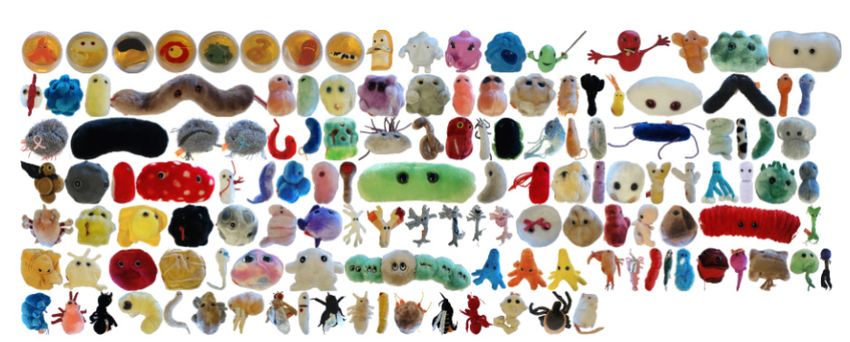
PREFACE

    This thesis presents original scholarship by the author. The results, analysis and views
reported throughout reflect work done largely by the author with assistance from Prof. Frank
Ferrie at McGill University.

                                             ii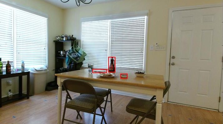
ACKNOWLEDGEMENTS

    Thanks to everyone in the Lab for useful discussions and inputs, namely: Michael, Amir,
Yan, Tony, Olivier and Prasun. Thanks to professor Ferrie for his guidance and allowing me
to explore a diverse topics during my time as a graduate student. Thanks to everyone in
McConnell 444 and also Seby for the interesting discussions on various topics in computer
vision. Lastly, thanks to Gilbert, ex-member of the Lab and ex-manager for pushing me to
achieve many goals during my work at 36Pix, which ultimately made me grow as an engineer.

                                            iii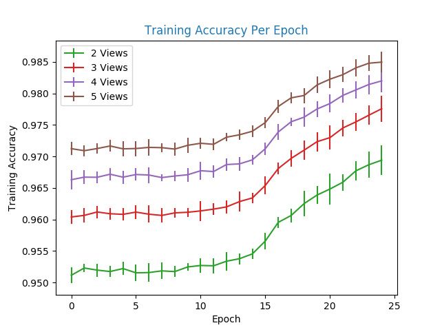
ABSTRACT

    In this work, we examine the literature of active object recognition in the past and
present. We note that methods in the past used a notion of recognition ambiguity in order
to motivate an agent to move the camera in order to take more views and disambiguate the
object. Present methods on the other hand are using deep reinforcement learning to learn
camera movement policies from the data. We show on a public dataset, that reinforcement
learning methods are not superior to a policy of adequately sampling the object view-sphere.
Instead of focusing on finding the next best view of the camera, we examine a recent method
of quantifying recognition uncertainty in deep learning and its potential application to active
object recognition. We find that predictions with this technique are well calibrated with
respect to the performance of a network on a test-set. However, we find no evidence that
this method can offer better results than directly looking at the network’s confidence in order
to gauge uncertainty in a rudimentary active object recognition experiment.

                                              iv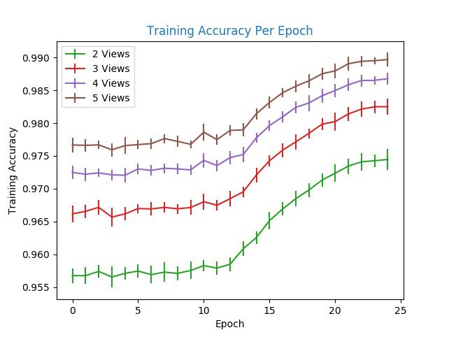
ABRÉGÉ

    Dans ce travail, nous examinons la littérature sur la reconnaissance active d’objets dans
le passé et présent. Nous notons que les méthodes utilisées dans le passé utilisaient la notion
d’ambiguïté de reconnaissance afin de motiver un agent à déplacer la caméra afin de prendre
plus de vues et de lever l’ambiguïté de l’objet. Les méthodes actuelles, en revanche, utilisent
l’apprentissage par renforcement en profondeur pour apprendre les règles de mouvement
de la caméra à partir des données. Nous montrons sur un ensemble de données public
que les méthodes d’apprentissage par renforcement ne sont pas supérieures à une politique
d’échantillonnage adéquat de la sphère de vue de l’objet. Au lieu de nous concentrer sur la
recherche de la meilleure vue possible de la caméra, nous examinons une méthode récente de
quantification de l’incertitude de reconnaissance dans l’apprentissage en profondeur et de son
application potentielle à la reconnaissance active d’objet. Nous trouvons que les prédictions
avec cette technique sont bien calibrées en ce qui concerne les performances d’un réseau sur
un ensemble de tests. Cependant, nous ne trouvons aucune preuve que cette méthode puisse
offrir de meilleurs résultats que d’utiliser directement la confiance du réseau afin de jauger
les incertitudes d’une expérience de reconnaissance d’objet actif rudimentaire.

                                              v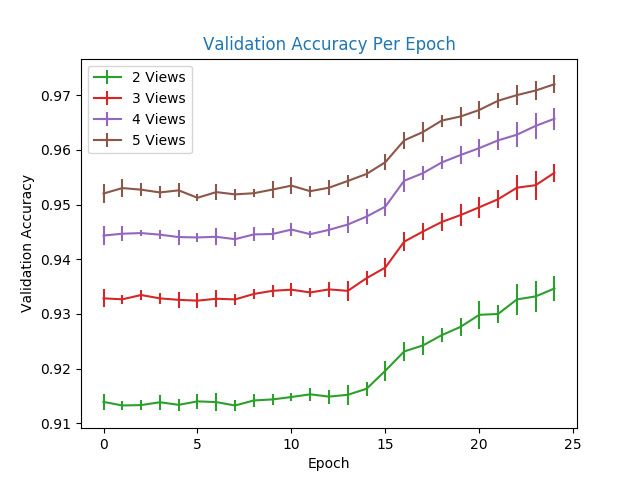
TABLE OF CONTENTS

PREFACE . . . . . . . . . . . . . . . . . . . . . . . . . . . . . . . . . . . . . . . . .           ii
ACKNOWLEDGEMENTS . . . . . . . . . . . . . . . . . . . . . . . . . . . . . . . .                   iii
ABSTRACT . . . . . . . . . . . . . . . . . . . . . . . . . . . . . . . . . . . . . . . .           iv
ABRÉGÉ . . . . . . . . . . . . . . . . . . . . . . . . . . . . . . . . . . . . . . . . . .          v
LIST OF TABLES . . . . . . . . . . . . . . . . . . . . . . . . . . . . . . . . . . . . .          viii
LIST OF FIGURES . . . . . . . . . . . . . . . . . . . . . . . . . . . . . . . . . . . .            ix
KEY TO ABBREVIATIONS . . . . . . . . . . . . . . . . . . . . . . . . . . . . . . .                 xi
1    Introduction . . . . . . . . . . . . . . . . . . . . . . . . . . . . . . . . . . . . . .       1
     1.1    Motivation . . . . . . . . . . . . . . . . . . . . . . . . . . . . . . . . . . .        1
     1.2    Overview of this Work . . . . . . . . . . . . . . . . . . . . . . . . . . . .           2
2    Literature Review . . . . . . . . . . . . . . . . . . . . . . . . . . . . . . . . . . .        4
     2.1    Active Object Recognition . . . . . . . . . . .      . . . . . . . . . . . . . . .      4
     2.2    Convolutional Neural Networks (CNNs) in the          Context of Active Object
              Recognition . . . . . . . . . . . . . . . . . .    . . . . . . . . . . . . . . .     12
            2.2.1 Object Recognition Using CNNs . . . .          . . . . . . . . . . . . . . .     12
            2.2.2 Capturing Classification Uncertainty . .        . . . . . . . . . . . . . . .     13
     2.3    Datasets . . . . . . . . . . . . . . . . . . . . .   . . . . . . . . . . . . . . .     16
3    Methodology . . . . . . . . . . . . . . . . . . . . . . . . . . . . . . . . . . . . .         19
     3.1    Reinforcement Learning for Active Object Recognition . . . . . . . .            . .    19
            3.1.1 Summary of the Reinforcement Learning Method by Malmir et                 al.
                     [30] . . . . . . . . . . . . . . . . . . . . . . . . . . . . . . . .   . .    19
     3.2    MC-Dropout for Active Object Recognition . . . . . . . . . . . . . . .          . .    21
            3.2.1 Motivation . . . . . . . . . . . . . . . . . . . . . . . . . . . . .      . .    21
            3.2.2 Experimental Setup . . . . . . . . . . . . . . . . . . . . . . . .        . .    22
            3.2.3 Probability Calculation and Uncertainty Measurements . . . .              . .    25
            3.2.4 Reliability Graphs and Calibration Error . . . . . . . . . . . .          . .    27
            3.2.5 Simple Active Vision Scenario . . . . . . . . . . . . . . . . . .         . .    28

                                                vi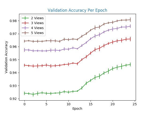
4    Results and Discussion . . . . . . . . . . . . . . . . . . . . . . . . . . . . . . . .   30
     4.1    Investigation of Reinforcement Learning Benchmark in [30] . . . . . . . .         30
     4.2    Experiments on the Modelnet Dataset . . . . . . . . . . . . . . . . . . . .       39
            4.2.1 Overview . . . . . . . . . . . . . . . . . . . . . . . . . . . . . . . .    39
            4.2.2 Training Details and Results for Networks Used in Modelnet Dataset          39
            4.2.3 Reliability Graphs, Expected and Maximum Calibration Error . .              40
            4.2.4 Simple Active Vision Scenario Results . . . . . . . . . . . . . . . .       45
5    Conclusion and Future Work . . . . . . . . . . . . . . . . . . . . . . . . . . . . .     50
Appendix A      Additional GERMS Results for the Right Arm . . . . . . . . . . . . .          53
REFERENCES . . . . . . . . . . . . . . . . . . . . . . . . . . . . . . . . . . . . . . .      57

                                              vii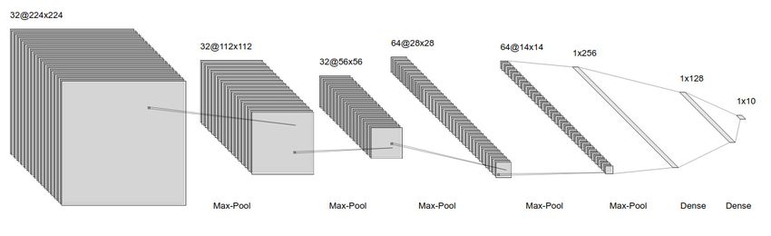
LIST OF TABLES
Table                                                                                          page
  4–1 The classification accuracy of various algorithms in the literature on the
        GERMS dataset over 5 views, compared to our Large Step Policy that
        adequately samples the viewsphere of the object, for the left arm of the robot. 38
  4–2 The classification accuracy of various algorithms in the literature on the
        GERMS dataset over 5 views, compared to our Large Step Policy that
        adequately samples the viewsphere of the object, for the right arm of the
        robot. . . . . . . . . . . . . . . . . . . . . . . . . . . . . . . . . . . . . . . .     38
  4–3 Classification Accuracy of the Models for Half the Training Data and All the
        Training Data on the Modelnet Test Set. . . . . . . . . . . . . . . . . . . .            40
  4–4 Expected Calibration Error and Maximum Calibration Error for a Standard
        CNN and a CNN Trained with Dropout. . . . . . . . . . . . . . . . . . . .                45
  4–5 The accuracy in picking the view giving the correct recognition from pairs of
        random views for the Modelnet dataset, where for each object we take 50
        random view pairs. . . . . . . . . . . . . . . . . . . . . . . . . . . . . . . .         49

                                              viii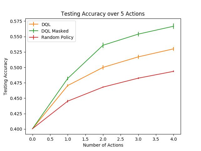
LIST OF FIGURES
Figure page
2–1 Objects used in the experiments of [5] . . . . . . . . . . . . . . . . . . . . . . 10
2–2 Objects used in the experiments of [30], [29], [19], [28] . . . . . . . . . . . . . 11
2–3 Objects used in the experiments of [35] . . . . . . . . . . . . . . . . . . . . . 11
2–4 Example scene from the Active Vision dataset presented in [2] . . . . . . . . 17
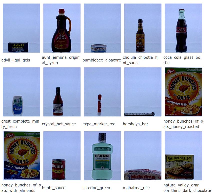
2–5 A subset of object instances from the Active Vision dataset presented in [2] . 18
3–1 Overview of the Method Presented in [30] . . . . . . . . . . . . . . . . . . . . 21
3–2 The set of views for an object in category bathtub. . . . . . . . . . . . . . . 23
3–3 The set of views for an object in category chair. . . . . . . . . . . . . . . . . 24
3–4 Model architecture for CNN-A and BNN-A. The only difference between the
two networks is that the latter has Dropout applied to it after every layer. 25
4–1 Training Loss per Epoch for the Left Arm . . . . . . . . . . . . . . . . . . . 32
4–2 Validation Loss per Epoch for the Left Arm . . . . . . . . . . . . . . . . . . 33
4–3 Testing Recognition Accuracy over 5 Views for the Left Arm . . . . . . . . . 34
4–4 Testing Recognition Accuracy over 5 Views for the Right Arm . . . . . . . . 35
4–5 Training Recognition Accuracy per Epoch for the Left Arm . . . . . . . . . . 36
4–6 Validation Recognition Accuracy per Epoch for the Left Arm . . . . . . . . . 37
4–7 Accuracy over 100 epochs for BNN-A with full training views (top) and half
the training views (bottom) . . . . . . . . . . . . . . . . . . . . . . . . . . 41
4–8 Accuracy over 100 epochs for CNN-A with full training views (top) and half
the training views (bottom) . . . . . . . . . . . . . . . . . . . . . . . . . . 42
4–9 Loss over 100 epochs for BNN-A with full training views (top) and half the
training views (bottom) . . . . . . . . . . . . . . . . . . . . . . . . . . . . 43
4–10 Loss over 100 epochs for CNN-A with full training views (top) and half the
training views (bottom) . . . . . . . . . . . . . . . . . . . . . . . . . . . . 44
ix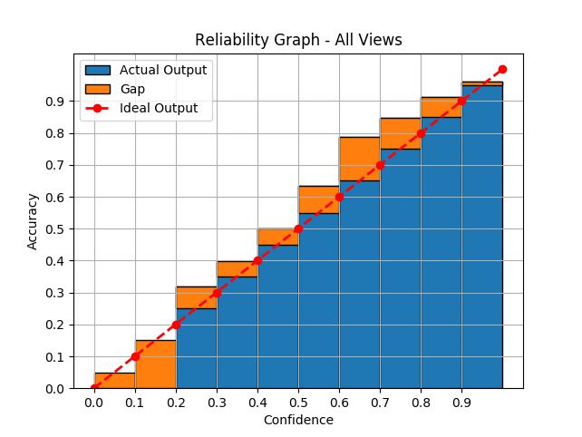
4–11 Reliability Graphs for CNN-VGG (top) and BNN-VGG (bottom) for all
       training data . . . . . . . . . . . . . . . . . . . . . . . . . . . . . . . . . .   46
4–12 Reliability Graphs for CNN-A for all training data and half training data . .         47
4–13 Reliability Graphs for BNN-A for all training data and half training data . .         48
A–1 Training Loss per Epoch for the Right Arm . . . . . . . . . . . . . . . . . . .        53
A–2 Validation Loss per Epoch for the Right Arm . . . . . . . . . . . . . . . . . .        54
A–3 Training Recognition Accuracy per Epoch for the Right Arm . . . . . . . . .            55
A–4 Validation Recognition Accuracy per Epoch for the Right Arm . . . . . . . .            56

                                            x
KEY TO ABBREVIATIONS
BNN : Bayesian Neural Network
CAD : Computer Aided Design
CNN : Convolutional Neural Network
COIL : Columbia University Image Library
ECE : Expected Calibration Error
HMM : Hidden Markov Model
KL : Kullback-Leibler
MCE : Maximum Calibration Error
RBF : Radial Basis Function
ReLU : Rectified linear Unit
SIFT : Scale Invariant Feature Transform
VGG : Visual Geometry Group
xiChapter 1
Introduction
1.1 Motivation
As computer vision systems based on deep learning are increasingly used in everyday
life, including safety critical applications such as autonomous driving, research needs to be
focused on evaluating and improving their robustness in face of unexpected input, which may
lie away from the data these systems were trained on. This unexpected input can be due to
various reasons such as uninformative view-points, bad lighting or weather conditions.
A common technique to deal with these challenges is data augmentation (creating more
data by processing existing data in some way) or simply collecting more data in a hope to
learn as many mappings as possible. However, in many practical applications, there are
limitations on how much data we can actually acquire or how much data augmentation can
help our cause.
Bad lighting for example, could cause an occluding effect on the object of interest.
Given that the light source and object can have an arbitrary relationship, it is unrealistic to
expect that we can include all the lighting possibilities for all objects in the training data,
by augmenting or otherwise collecting data with all possible lighting conditions.
When it comes to viewpoint, consider the simple example of a cup and a pan. Seen
from the top, a cup shares many common features as the pan, however it is hard to mistake
a pan as a cup from most other views. In this case, features of two different objects are
similar from a subset of viewpoints, while very different in other viewpoints. It is unrealistic
to think that we can train all objects from all different viewpoints, not only because the data
acquisition is hard, but also because even if we could, it is inevitable that some objects will
have similar features at different viewpoints.
1Furthermore, in situations where we have very little data in training and certainly not
enough data to adequately sample all the viewpoints of an object, it is important to know
when the network is unsure of its answer and acquire more data in order to disambiguate
the object.
The essential problem we are dealing with is a recognition ambiguity. We know from
information theory that by acquiring more informative data we can reduce this ambiguity.
Thus, this suggests an active vision solution, where an agent controls the camera and gathers
more data in order to reduce recognition ambiguity. By using this extra information, we can
also hopefully provide some guarantees as to the quality of our classification. Given that
this is a broad problem, we will focus on recognition ambiguity as a result of uninformative
view-points.
In particular, we will examine the current and historical literature on active object
recognition and show that finding the next-best-view, as the problem is currently framed,
is of less importance than evaluating the quality of the recognition at each time-step. We
will explore a recent technique of obtaining uncertainty estimates in the context of deep
networks and attempt to evaluate the quality of those uncertainty estimates in an active
vision scenario. Our goal is to determine whether this technique yields a better quantification
of uncertainty in the face of unexpected input, compared to simply taking the output of the
Softmax of a standard network.
1.2 Overview of this Work
This work is organized as follows: in Chapter 2 we first review the Active Object Recog-
nition literature from the early work to modern attempts using deep learning approaches
in Section 2.1, which focus mainly on Next-Best-View (NBV) prediction. Then, in Sec-
tion 2.2 we discuss Convolutional Neural Networks (CNNs) in the context of active object
recognition. Namely, although CNNs can be powerful enough to dispense for the need of
a sophisticated NBV strategy, the actual challenges relate to the fact that the output of
the CNN can be not informative as a metric to quantify recognition uncertainty. Lastly,
2in Section 2.3 we describe the various datasets used in the recent literature, as a way to
benchmark active object recognition algorithms.
In Chapter 3, we discuss the experimental setup. In Section 3.1 we discuss the experi-
mental setup of a work in the existing literature that proposed a reinforcement learning NBV
policy. In Section 3.2 we discuss the experimental setup for evaluating different signals to be
used as part of the feedback loop in an active vision scenario. In Chapter 4, we discuss the
results of the experiments described in Chapter 3. Specifically, in Section 4.1 we discuss the
results obtained in the experiment described in Section 3.1, while in Section 4.2 we discuss
the results in the experiment described in Section 3.2.
Lastly, in Chapter 5 we summarize the insights gained by examining the current liter-
ature and from the results of the experiments comparing the different output signals. We
finally offer some ideas for future work to extend this investigation.
3Chapter 2
Literature Review
2.1 Active Object Recognition
Active vision approaches have a rich history in the computer vision literature. Aloi-
monos, who popularized the term Active Vision, showed that a number of low level vision
problems such as shape from shading, depth computation, shape from texture and struc-
ture from motion that are ill-posed for a passive observer, are simplified when addressed by
an active observer [1]. In this section however, we will focus on active object recognition
approaches.
Bajcsy introduces the concept of active perception as using an intelligent controlling
strategy to guide the data acquisition process [3]. That strategy, she argues, requires measure
parameters and errors from the scene to be fed back in order to guide the data acquisition
process. Thus, instead of trying to improve imperfect data, that imperfect data can be used
to change the sensor state parameters. Wilkes and Tsotsos [44] apply this concept to the
task of object recognition. In their work, they show that by using a mobile camera they can
overcome difficulties due to variations such as changes in imaging geometry and illumination
by driving a mobile camera to a standard view, using a tree-based indexing scheme. The
system is tested on a set of 8 origami objects.
In line with Bajcsy’s ideas of using errors from the scene in order to guide a data
acquisition process, Callari and Ferrie’s method for view selection uses scene ambiguity due
to noisy measurements and uncertain models in order to efficiently gather new data [5]. In
fact, their work was inspired by and largely based on Whaite and Ferrie’s earlier work [43],
where they propose an autonomous exploration technique to model volumetric shapes. The
central idea behind Whaite and Ferrie’s technique was to take measurements wherever the
predicted uncertainty in model parameters was the largest, thus maximizing the information
4gain in model parameters. Extending this work for active object recognition, Callari and
Ferrie [5] showed that taking measurements in areas with largest predicted uncertainty is
not sufficient for the object recognition task, since these areas can lie parallel to the inter-
class decision boundary. Thus, the relationship between measurement location and inter-
class decision boundary must be taken into account as well in order to optimally guide the
autonomous agent. It is important, for later discussion, to note that the precise definition
of the recognition ambiguity in this work is the Shannon entropy of the posterior object
distribution, and the information gain across two successive views simply the difference in
entropy of the first view minus the second view.
Following in the footsteps of the work in [44], Dickinson and Tsotsos [7] expand on
the ambiguities inherent to single view recognition, including the impossibility of inverting
projection, problems with feature detectability and view degeneracies. They use a Bayesian
based attention mechanism that performs a probabilistic search through a hierarchy of fea-
tures such as geon primitives, faces and boundary groups in order to guide the camera
to a new viewpoint whenever the features recovered do not provide a unique mapping to
an object. The main driving force of the active recognition framework are the conditional
probabilities that the authors extract by sampling geons from a Gaussian sphere.
The Shannon entropy as a measure of object recognition uncertainty in the context of
probabilistic object recognition is also used by [38] , where they use concepts from infor-
mation theory for their active object recognition algorithm in order to determine the most
discriminant viewpoint. The main idea is to use receptive field histograms in order to rep-
resent the appearance of each object and then greedily select views in order to reduce the
information-theoretic uncertainty of the category hypothesis.
Paletta and Pinz are the first to introduce reinforcement learning techniques in the
context of active recognition [35] in 2000, long before the recent resurgence in interest in the
topic. In their paper they describe how reinforcement learning can be used in order to learn
the strategy for efficient exploration, thus dispensing the need for explicit reasoning-based
5viewpoint planning such as in [38] and [5]. In particular, they use Q-Learning with an RBF
neural network where the reward depends on the information gain defined as the reduction of
Shannon entropy between two successive views. With the Q-Learning approach the actions
taken by the agent are those that are determined to maximize the expected reward, in this
case the actions that minimize the Shannon entropy.
In the robotics literature we have methods such as the one by Browatzki et al. [4] who
develop a technique for active object recognition on a humanoid robot, using particle filtering
for object exploration based on color features that is tested on 5 cups with different color tape
taped at the bottom. There is also the work by Potthast et al. [37], who extract SIFT features
from the image and then use those features as an input to a Hidden Markov Model (HMM)
that estimates the recognition state and a next viewpoint selection strategy dependent on the
expected loss of entropy. These techniques are motivated more by computational constraints
and simple practical applications.
At this point, it becomes pertinent to discuss the reason why there was such extensive
work on finding the most discriminant view in the early literature. The object recognition
methods of that era were a lot more error prone than modern methods based on deep
convolutional neural networks. As Dickinson notes : "degenerate views occupy a significant
fraction of the viewing sphere surrounding an object" [8]. However, as we will see in Section
2.2 and Section 3, convolutional neural networks do not appear to suffer from the same
limitations for a large class of problems due to the rich feature hierarchy they learn and
the effect of pooling. On the other hand, it is more difficult to evaluate the quality of their
recognition in order to use errors as part of a feedback model to acquire new views.
End-to-end methods using deep networks have been proven tremendously successful in
many computer vision tasks such as object recognition, semantic segmentation and object
detection. In fact, much of the recent literature in computer vision has been focused on deep
learning methods including the, relatively sparse, literature on active object recognition.
Thus, more recent attempts on active object recognition resemble that of Paletta and Pinz
6[35]. However, despite the resemblance to [35], the interest in using reinforcement learning for
view planning can be traced to the famous "Playing Atari with Deep Reinforcement Learn-
ing" paper by DeepMind [31]. The challenges of using Deep Learning methods (stochastic
gradient descent on a neural network) for reinforcement learning include the fact that data
samples are not independent, but actually highly correlated, while the distribution changes
over time. This violates the assumptions used when training neural networks with stochastic
gradient descent. The paper describes simple practical methods to overcome these problems,
namely experience replay and epsilon-greedy exploration. This makes training stable and
shows how the benefits of deep learning (ability to learn complex mappings while maintaining
good generalization) can be extended to the domain of optimal policy selection.
Following that breakthrough in reinforcement learning research, the recent papers [30]
[29] [2] [28] on active object recognition almost exclusively use variants of reinforcement
learning to learn control policies end-to-end , while [19] uses recurrent neural networks, still
learning the control policy end-to-end. Learning an end-to-end policy using reinforcement
learning or other learning methods requires a large amount of data, thus along with their
methods, [30] and [2] present relatively large scale datasets in comparison to the ones used
in the past. The datasets, as well as their limitations will be discussed more in detail in
Section 2.3.
The method described in [30] is based on Q-Learning and is evaluated on the GERMS
dataset, which is introduced in the same paper. In particular, a VGG-16 CNN is used
to classify the objects in a set of probabilities through the softmax layer, in this case 136
probabilities each representing a given class. The state of the system Bt is defined as Bt =
O1 ∗ O2 ∗ ...Ot , where Oi is the softmax output at the current timestep. Recognition is done
after a pre-defined number of moves determined by performance on the validation set, in
this case 5 moves. The output class c is simply argmaxc (Bt ). The camera movements are
determined by an action network that outputs the most optimal action, which is the action
with the highest Q-value at the current state. The Q-value Q(s, a) for each action at each
7state is learned through training the action network using standard reinforcement learning
techniques. The method will be described in more detail in Section 3.1. In [29] they train
both the recognition and action model end-to-end and evaluate various ways to integrate the
belief of the system on its prediction at each timestep, achieving slightly higher recognition
rates than their work in [30].
Ammirato et al. [2] introduce another dataset along with their method. Their method
however is very similar to the one in [30] in that an action network is optimized to produce a
next-best-view action, where the state of the system depends on the output of a convolutional
network. Instead of using the output of the softmax, they use an N-dimensional feature vector
extracted by a convolutional network as the state. Instead of using Q-Learning, they use the
REINFORCE algorithm [45] to train their action network.
Lastly,[19] train four modules end-to-end in order to produce the next-best-view action
and validate their method on the GERMS dataset. The modules used are an actor, sensor,
aggregator and classifier models, which are all neural networks that have different roles. The
sensor module produces a feature vector that is fed to the aggregator that produces an ag-
gregated feature vector taking into account feature vectors produced in previous timesteps.
The classifier module classifies the object at a given timestep and the actor module produces
a next-best-view based on the aggregated feature vectors. All modules are trained using
stochastic gradient descent, while the actor network is trained using the REINFORCE al-
gorithm [45]. The central idea behind the paper is to let a network learn four important
functionalities of an active object recognition system, namely how to classify the objects,
which features from the image to use, how to integrate the features over time and what the
next-best-view should be. This is a symptom of the times, where computer vision tasks are
left to a neural network, without an effort to understand the underlying laws that govern
recognition.
The method described in [20] is one exception to the use of reinforcement learning vari-
ants for next-best-view prediction. The main idea is to use Convolutional Neural Networks
8to perform trajectory optimization, by decomposing an image sequence into image pairs
and mapping directly from observation to new viewpoints. They render grayscale images
around the view sphere of 3D CAD meshes in the Modelnet dataset [21] and create a set of
M (M −1)
N = 2
view pairs for a sequence of M views to explore. They use a Siamese CNN,
which is two CNNs that have shared weights, to compute a class probability distribution for
each view pair. Following that, a second CNN is trained to output the best viewpoint to
move to for any given image. To train the second CNN, they use the output of the first CNN
for the view-pair associated with a given training image xk that gives the highest output for
the ground truth class, with the label being the relative pose. At test time, a single image is
passed through the second CNN which outputs the next-best-view. Lastly, in order to take
into account all images in the trajectory, a third CNN is trained to map a single image to a
distribution of predicted cross-entropies around the view sphere in order to find a trajectory
with the minimum sum of cross-entropies. The problem with this approach is that it treats
the classification output of the CNN as a valid probability distribution, which as we will see
in Section 2.2.2 is not the case.
At this point it becomes pertinent to compare and contrast the methods seen in the
literature. Early methods such as [7], [5], [38], use principled scientific methods based on
errors present in the scene to guide the agent. The authors make an effort to understand
how and where the object recognition methods of that time fail. On the other hand, recent
methods based on reinforcement learning make little effort to assess those errors and recog-
nition failure modes and let the action network decide on what to use in order to drive the
agent. Thus, the only assessment on the quality of recognition comes through metrics on
a test set, which does little to increase understanding of what can go wrong in single view
recognition using modern convolutional neural networks.
Due to computational constraints of that time along with the constraints of object
recognition methods back then, the experiments are done on a small scale with relatively
simplistic objects. For example, [5] use a simple set of clay objects to validate their method as
9depicted in Figure 2–1, while [35] validate their method on a set of 16 objects shown in Figure
2–3. The small scale of the experiments and the fact that many of the datasets used are
proprietary, makes it difficult to compare and evaluate these methods. One exception is [38],
who used the publicly available Columbia University Image Libracy (COIL-100) dataset [33]
containing 100 objects sampled every 5 degrees of rotation on a turn-table. Recent methods
use relatively large scale datasets that were developed to train the agent. For example, [30],
[29], [28] and [19] all validate their methods on the GERMS dataset [30] that contains 136
objects in 816 training and 549 testing tracks, where each track has 145 ± 12 annotated
frames. The objects used in the datasets are quite complex as shown in Figure 2–2 and the
fact that the data as well as the environment are publicly available helps benchmark and
compare different methods.
Figure 2–1 – Objects used in the experiments of [5]
The main weakness of deep reinforcement learning solutions is that they require a lot
of data in order to train the action network. This is hardly practical in many engineering
applications. In fact, one of the main reasons why actively controlling a sensor is necessary is
the fact that we might have inadequate sampling of the objects in question. These methods
are also system and dataset specific. An action network trained on a specific object - action
system is quite useless when either the objects or the system change, requiring a whole new
10Figure 2–2 – Objects used in the experiments of [30], [29], [19], [28]
Figure 2–3 – Objects used in the experiments of [35]
11data acquisition process to take place. On the other hand, methods in the past with the
exception of [35], did not rely on a network to make trajectory optimization decisions but
used feedback directly from the scene, which means that the general principles could be
used, in theory, for camera trajectory optimization in different environments and with other
objects without relying on expensive data acquisition.
2.2 Convolutional Neural Networks (CNNs) in the Context of Active Object
Recognition
2.2.1 Object Recognition Using CNNs
A detailed review of how Convolutional Neural Networks (CNNs) work in the context
of classification is out of scope for this work, but in this section we will review some of the
relevant aspects in regards to active object recognition.
Although there are an inexhaustible number of CNN variants in the literature, they
typically share the following layers : convolutional layers and pooling layers, along with a
non-linear activation layer [14], in a sequence whose depth and size depends on the specific
architecture.
The pooling layer, down samples the output of a layer by replacing each k x l neighbor-
hood of the feature map with its summary statistics [13], where the size of the neighborhood
depends on the specific network architecture. Max pooling, for example, replaces each k x l
neighborhood of values in the feature map with the maximum value of that neighborhood.
This creates invariance to small translations in the input. In fact, pooling can be thought
of an infinitely strong prior that each activation unit in the network should be invariant to
small translation [13].
To further understand how CNNs work and gain intuition regarding their operation we
can visualize the learned features. In their very influential paper, Zeiler and Fergus [47] use
a deconvolutional network to map the activities of intermediate layers to the input pixel
space, thus being able to visualize which pattern in the image activates each feature map.
The features learned by the CNN are determined to be hierarchical in nature, increasing in
12their complexity the deeper in the network they are. They show that the second layer of the
network responds to corners, edges and colors, the third layer to textures while the last two
layers are class specific, responding to complex patterns such as faces and even entire objects.
One of the most important conclusions, which is related to active object recognition is that
small transformations in the input image have a dramatic effect in the first layer’s features,
but less impact on the abstract feature layers, thus rendering the network largely invariant to
translation and scaling of the input. Therefore, if an abstract feature used for classification
is present anywhere in the image, the network’s output is not likely to be affected.
A more recent and very popular technique of visualizing which parts of an image influ-
ence classification is introduced by Selvaraju et al. [39], which unlike the method in [47],
does not require a deconvolution network while the visualizations are class discriminative.
The technique uses the gradient passed to the last convolutional layer after a classification
and passes it back to the input space by backpropagation in order to visualize which part of
the input affects classification. By using this technique one can gain an intuition behind a
network’s decisions, without the need of making any modifications to the network structure.
The aforementioned techniques are useful in terms of gaining intuition regarding the
failure modes due to self-occlusion that we are trying to overcome with active object recog-
nition. They do not provide however a usable signal on which to base an active recognition
algorithm since they are purely for visualization purposes.
2.2.2 Capturing Classification Uncertainty
As we saw in Section 2.1, a core theme in the early active vision literature is using errors
from the scene as a signal to a feedback mechanism that guides an intelligent data acquisition
strategy. Although the models used for object recognition were fairly weak compared to
CNNs, they provided signals in the form of uncertainty that could be used as a part of an
active recognition strategy. A common mistake of engineers that do not have experience with
deep networks is to try to interpret the output probability of a softmax layer as a meaningful
13probability distribution that conveys the network’s confidence on each class. In this section
we will see that this is not the case both by theoretical and experimental work.
Back in 2005, Niculescu et al. [34] showed that neural networks provide well calibrated
predictions. In a multi-class classification setting, perfectly calibrated predictions are defined
as:
P (Ŷ = Y |P̂ = p) = p, ∀p ∈ [0, 1] (2.1)
Where Y is the label, Ŷ is the prediction and P̂ its confidence. In practical terms, we
want given 100 predictions each with confidence 0.8, that 80 are correctly classified. However,
Guo et al. [16] show that modern deep networks, including CNNs, are not well calibrated.
In fact, networks tend to have overconfident predictions, even if they are wrong.Thus, the
confidence of a network to its prediction cannot be reliably used as part of an active vision
strategy.
Having established that the output of the Softmax layer is not useful in an active
vision strategy from an empirical standpoint, we can go into more detail of why this is
the case. Deep networks and by extension CNNs provide only a point estimate of weights
and predictions [13], that can be accurate within the confines of the data distribution that
the network was trained on [9]. Unlike Bayesian Neural Networks (BNNs) that contain
uncertainty information in their predictions, deep networks provide deterministic function
approximations [9]. In fact, when deep networks are faced with unexpected input, in our
case an unexpected viewpoint or occlusion, the behaviour of the network is undefined and
can output any value with any confidence. With BNNs, given training data X with labels Y ,
Bayesian Inference is used to compute the posterior distribution over the weights of a network
p(W |X, Y ), which captures the distribution of model parameters that could explain the data
and therefore allow us to compute the model uncertainty on its prediction. By placing a
prior distribution over the weights p(W ), we can use Bayes theorem to evaluate this posterior
p(Y |X,W )p(W )
as p(W |X, Y ) = p(Y |X)
. However, calculating the posterior for complex models is
14intractable due to the p(Y |X) term. In the BNN literature, there are various approximate
inference techniques to estimate it by learning a simpler approximate distribution q(W ) and
minimizing the Kullback-Leibler divergence between this approximate distribution and the
true posterior:
q(W ) = argminq(W ) KL(q(W )||p(W |X, Y )). (2.2)
But so far, BNNs have limited practicality in engineering applications compared to deep
networks[9].
Gal and Ghahramani [10] provide a practical method to obtain uncertainty estimates in
networks that provide state-of-the-art results in various applications, including CNNs. They
show that training a network with stochastic regularization techniques such as Dropout
[40] applied to it at every layer during training with a cross-entropy loss, is equivalent to
minimizing the KL-divergence between q(W) and the true posterior in Equation 2.2. At
test time, using Monte Carlo sampling with T stochastic forward passes over the network
with Dropout, uncertainty estimates can be obtained using well known methods such as the
Shannon entropy and variation ratios for classification tasks.
In followup work Kendall and Gal discuss the types of uncertainty estimates needed
for computer vision applications [24]. They describe the two major types of uncertainty as
aleatoric and epistemic uncertainty. Aleatoric uncertainty relates to the noise in the data,
while epistemic uncertainty relates to the uncertainty of the model in its predictions. They
observe that modeling epistemic uncertainty is most useful in low data regimes, as it can
capture out of distribution examples. This epistemic uncertainty can be captured simply
by training a network with Dropout and performing T stochastic passes with Dropout still
on in testing[23]. This method of obtaining uncertainty estimates will be henceforth refered
to as MC-Dropout. They provide experimental results in semantic segmentation and pixel-
wise depth regression, showing that by explicitly modelling uncertainty there is a 1% to 3%
improvement on existing methods.
15Gal’s method for estimating uncertainty has found a wide range of applications in the
literature, including semantic segmentation [22], pose estimation [23], active learning [11]
and medical imaging [27]. In Section 4.2 we will attempt to experimentally validate whether
or not this uncertainty information can be used as a signal in an active object recognition
strategy.
2.3 Datasets
The datasets used to develop and test active object recognition approaches in the early
literature are simplistic and small by today’s standards. Other recent methods, such as [37]
use small proprietary table top datasets. In the recent literature, there are three public
datasets that could be useful in developing and benchmarking active vision techniques using
deep learning methods, the GERMS dataset [30], the Active Vision dataset presented in [2]
and finally the ModelNet dataset [46] which contains CAD models.
The GERMS dataset contains 136 objects as shown in Figure 2–2 with 816 training video
tracks and 549 testing tracks of a robot handling the objects and rotating its wrist by 180
degrees as to actively examine them. The tracks are divided based on the arm of the robot,
with around half the training and testing tracks being the left arm and the other half the right
arm. In each clip the object is handed to the robot in one of 6 predetermined poses. In the
π
original work, the author allows rotations of ± , π, π
64 32 16
, π
8
and π
4
degrees, for a total of 10
possible moves, allowing both fine-grained inspection and large wrist movements. Although
this dataset is much larger than any other before it, it suffers from serious limitations. One is
that although there are around 22000 total images, the objects in both training and testing
are the same, just with a different starting position. Furthermore, the data is simply not
enough to train a CNN, which is why in their original work the authors just extracted features
with a pre-trained CNN and fine-tuned just the softmax layer in order to extract the use the
softmax probabilities as part of an active vision strategy.
The dataset presented by Ammirato et al. [2] contains 30000 RGBD images with 30
object instances. The dataset simulates motion of a robot that actively examines object
16instances in 15 different scenes. The authors provide bounding boxes for the instances in
question to simplify the recognition process. The simulated motions are a step up, down,
left and right as well as a clockwise and counter-clockwise rotation through the scene. An
example of the objects in the scene can be seen in Figure 2–4 and a subset of the instances
used in Figure 2–5. The dataset however has the same limitations as the GERMS dataset.
Although there are many images per sample covering several viewpoints, the number of
distinct samples are very few. The authors acknowledge in their paper that deep networks
can easily over-fit due to the small number of samples.
Figure 2–4 – Example scene from the Active Vision dataset presented in [2]
Lastly, there is the ModelNet dataset [46] which has 127915 CAD models from 662
categories. By rendering the CAD models it is straightforward to acquire grayscale images
around the view-sphere of each object. This dataset is by far the richest one in terms of
training and testing examples. However, the data tends to be a bit simplistic to the point
where existing methods [21] achieve up to 98% classification accuracy. Also, there is no color
information and categories tend to be quite distinct.
17Figure 2–5 – A subset of object instances from the Active Vision dataset presented in [2]
18Chapter 3
Methodology
3.1 Reinforcement Learning for Active Object Recognition
3.1.1 Summary of the Reinforcement Learning Method by Malmir et al. [30]
In this section we will explain the main ideas behind the method for next-best-view
selection presented in [30], which is based on Q-Learning. The main idea of the paper is
to use reinforcement learning to learn a policy that chooses the next-best-view for an agent
actively examining the object in order to maximize recognition accuracy with the fewest
number of steps.
The system architecture is based on the Figure 3–1. By fine-tuning the Softmax layer
of an AlexNet [25] network pre-trained on Imagenet for the GERMS dataset, the author
obtains a vector with dimensionality corresponding to the number of classes, which is 136
for this dataset. These outputs are included in the dataset presented in the same work, along
with the joint position of the robot.
Ot ∗Bt−1
At each timestep t, the state of the system is updated by the following rule Bt = Ot +Bt−1
,
where Bt is the state of the system and Ot is the softmax output at the view in timestep t.
This vector Bt becomes the input to the Action Network at the current timestep.
The Action Network is a standard fully connected neural network with ReLU activation
functions. The output of the network is a vector of Q-values, one for each action, for a total
of 10 values. At each timestep, the optimal action is determined to be the one with the
highest Q-value. The problem then becomes one of estimating the Q-value Q(s, a) of the
each action α at each state s. Thus, the iterative update for estimating Q(s, a) becomes:
Q(s, a) ← Q(s, a) + λ(R(s, a) + γ a Q(s , α ) − Q(s, a)) (3.1)
max
19Equation 3.1 is the classical Q-Value update rule described in [42]. It is a simple way
to learn optimal policies in a Markovian domain. The estimate of Q(s, a) is iteratively
improved using the current estimate, and the estimate of the optimal value of the next state
a Q(s , α ). The estimate update is scaled by the learning rate λ. R(s, a) is the reward,
max
in this case given to the agent if the recognition is correct. Lastly, γ denotes the discount
factor, which if set to be γ < 1, weighs down future rewards in favor of more short term
rewards.
The iterative weight update for a neural network with weights W with Bt being the
state then becomes:
∂
W ← W − λ(R + γ a Q(Bt+1 , a) − Q(Bt , at )) Q(Bt , at ) (3.2)
max ∂W
In practical terms, using the Keras machine learning package [6], a fully connected
neural network with three layers with 136, 512 and 10 units respectively is created, where
the first two layers are followed by a ReLU non-linearity, while the last layer is followed by
a Softmax. To get the weight update in Equation 3.2 using Keras automatic differentiation
the following Loss function is needed:
1
L(W ) = (R + γ a (Q(Bt , a) − Q(Bt , a))2 ) (3.3)
2N max
Here, Equation 3.3 is the square error loss between the largest Q-value of the next action
and the estimate of the highest Q value at the current timestep. The network is trained using
standard stochastic gradient descent.
To avoid repeated actions during training, - greedy exploration is used during training,
whereupon a random action is taken with probability .
20Figure 3–1 – Overview of the Method Presented in [30]
3.2 MC-Dropout for Active Object Recognition
3.2.1 Motivation
As will be shown in Section 4.1, the method proposed by Malmir et al.[30], as well
as other methods in the recent literature do not outperform a simple policy of adequately
sampling the view space of the object in the GERMS dataset by taking large steps and
naively integrating the Softmax outputs. So, instead of focusing on the next-best-view, in
this section we focus on the evaluation of feedback signals.
In an active recognition setting, it is important to have a reliable assessment of the
recognition uncertainty. This can prompt the agent to start taking new views and can also
be used to decide when to stop acquiring new views. It can also help when integrating
the information from different timesteps, weighing the predictions by their uncertainty for
example. Assuming we have a fixed policy of always moving the camera in one direction in
large steps, we would like to assess whether the method of obtaining uncertainty by using
Monte Carlo sampling of a network trained with Dropout as proposed by Gal et al. [10] is
useful in an active recognition scenario. The network trained in this fashion will henceforth
be referred to as BNN, while a standard network as CNN.
21Unfortunately, the GERMS dataset [30] and the Active Vision Dataset [2] do not provide
enough data to train a CNN network in a way to get these uncertainty estimates. In this
section, we will discuss the methodology behind the assessment of BNNs for active vision
using the Modelnet Dataset [46].
3.2.2 Experimental Setup
As described in Section 2.3 the ModelNet Dataset [46] comprises of 3D CAD meshes. To
render grayscale images we use perspective projection with objects scaled uniformly to fit the
viewing window and Phong shading [36]. We use the ModelNet10 subset of the dataset for
our experiments, containing 1000 objects with 12 views for each object, similarly to [20]. The
views are taken at an elevation of 30 degrees from the ground plane, with camera movements
of 30 degrees around the object for a total of 12 views for each object. An example is shown
in Figures 3–2 and 3–3. It is important to note that images are aligned. This means that, for
example, every chair in the dataset has the view at 0 degrees facing forward like the example
in Figure 3–3 and subsequently rotated clockwise 30 degrees at a time for every subsequent
view.
We experiment with two scenarios: one where we are allowed to train with full sampling
of the view-sphere and another where we only have access to half the views for training. The
first scenario attempts to assess whether using the uncertainty provided by BNNs is more
informative than the Softmax output of a standard CNN in disambiguating views that can
be confused with views of other objects. The second scenario deals with inadequate sampling
of the objects. We remove half the views from the training set of each object category so as
to bring certain viewpoints outside the training distribution. Since the dataset is aligned,
we completely eliminate half the view-sphere for each training object in a consistent way.
This means that all the images containing certain viewpoints, eg. a forward facing chair, are
eliminated from all objects in the training set. The three first views to be masked are chosen
at random for each object. The subsequent three views are those 180 degrees away from each
of the first three views. This is due to the fact that many objects are symmetric, such as
22Figure 3–2 – The set of views for an object in category bathtub.
23Figure 3–3 – The set of views for an object in category chair.
24the bathtubs in Figure 3–2. At test time, we evaluate whether the uncertainty estimates of
the BNN are better than the CNN output at predicting whether we are out of distribution,
in order to prompt the agent to acquire new views.
Two networks are used in the experiments, a network that has Dropout applied to it
after each layer, and a network where Dropout is applied only for regularization, which we
term as BNN-A and CNN-A respectively for the purposes of this work. These networks have
identical architecture with a small number of parameters due to the relatively small size of
the dataset. They comprise of 5 Convolutional layers, each followed by a pooling layer and
3 fully connected layers as in Figure 3–4.
Figure 3–4 – Model architecture for CNN-A and BNN-A. The only difference between the
two networks is that the latter has Dropout applied to it after every layer.
3.2.3 Probability Calculation and Uncertainty Measurements
Following the discussion in Section 2.2.2, we train BNN-A and CNN-A with a standard
cross entropy loss as in Equation 3.4, with L2-regularization applied to the weights to prevent
over-fitting due to the small size of the dataset. Then, by doing T stochastic forward passes
through the network with Dropout, we can approximate an actual probability distribution
for our prediction as a mean over the Softmax outputs [23], shown in Equation 3.5. Where
25Wt are the weights, y the output, T the number of stochastic passes through the network
and X the dataset with labels Y .
1
N
L(Wi ) = − logp(yi |f Wi (xi )) + ||Wi ||2 (3.4)
N i=1
1
T
p(y = c|x, X, Y ) = Sof tmax(f Wt (x)) (3.5)
T t=1
Lastly, since we get an approximation of the true probability with Equation 3.5, we can
use standard ways of quantifying uncertainty. In our experiments, we use the uncertainty
measures proposed by Gal in [9] for classification tasks, namely Variation Ratios, Shannon
Entropy and Mutual Information described below.
The calculation of the Variation Ratio is shown in Equation 3.6, where T is, again, the
number of stochastic forward passes through the BNN, 1 the indicator function and c the
mode of the predicted class over the T forward passes. Lastly, ŷ denotes the prediction,
given input x and dataset X with labels Y .
T
t=1 1[yt = c]
variation − ratio[ŷ|x, X, Y ] = 1 − (3.6)
T
The Shannon Entropy H is approximated as in Equation 3.7, where we simply use
Equation 3.5 as a probability approximation.
1 1
T T
H[ŷ|x, X, Y ] ≈ − p(yt |x, Wt )log( p(yt |x, Wt )). (3.7)
T t=1 T t=1
Lastly, we can also approximate the Mutual Information of our T predictions by sub-
tracting the entropy from the entropy expectation over all T predictions as in Equation
3.8.
M I[ŷ, W |x, X, Y ] ≈ H[ŷ|x, X, Y ] − E[H[ŷ, W ]]. (3.8)
26The difference between Mutual Information and the other metrics is that Mutual In-
formation can capture the model’s confidence in its output, while Shannon Entropy and
Variation Ratios capture the uncertainty in the prediction [9]. For example, in a scenario
where a CNN outputs the same prediction in a binary classification task with the output
y = 0.5 for all T stochastic passes through the network, Shannon Entropy and Variation
ratios would indicate high uncertainty, while Mutual Information would output high confi-
dence, since it measures the model’s consistency in its prediction.
3.2.4 Reliability Graphs and Calibration Error
The output of a network is defined as perfectly calibrated if Equation 2.1 holds. Any
deviation from Equation 2.1 is defined as the miscalibration of the network predictions. In
an active vision scenario we would like the network’s predictions to have minimal calibration
error, so we can use the output confidence in order to make decisions on whether to take
a next view. We hypothesize that the output probability computed by Equation 3.5 for
BNN-A, would exhibit lower calibration error than the Softmax output of CNN-A. We also
hypothesize that as certain viewpoints become out of distribution in the low data scenario,
the miscalibration increases. However, we also hypothesize that the miscalibration for this
scenario would be lower in the case of BNNs, because epistemic uncertainty is supposed
to be able to capture the model’s uncertainty in data it has not trained on. In order to
test the above hypotheses, we use reliability graphs [34] to visualize the calibration error
and Expected Calibration Error (ECE) and Maximum Calibration Error to quantify the
miscalibration (MCE) [32].
The reliability graph [34] shows the accuracy versus confidence of the predictions. Specif-
1
ically, we place the predictions into N bins of size , where in our case N = 10. Then,
N
n−1 n
bin Bn contains the predictions that have confidence between and . The accu-
N N
racy of bin Bn is simply the accuracy of the predictions contained within: acc(Bn ) =
1
1(ŷi = yi ). Similarly, the confidence of each bin is the average confidence in
|Bn | i∈Bn
271
that bin con(Bn ) = p̂i . For perfectly calibrated predictions, it is evident that the
|Bn | i∈Bn
graph would represent the identity.
The reliability graph described above is a good visualization tool but it does not provide
useful metrics. Thus, we calculate scalar summaries of the miscalibration, in the form of
the Expected Calibration Error (ECE) and Maximum Calibration Error(MCE) [32], which
also involve binning. The expected calibration error approximates the expected difference
between accuracy and confidence. It does so by computing the weighted average of the
absolute difference between the networks average accuracy at each bin with its average
|Bn |
confidence : ECE = N n=1 |acc(Bn ) − conf (Bn )|. Lastly, MCE calculates the maximum
n
error encountered in any bin Bn , which could be important for safety critical applications.
Thus, M CE = maxn∈1,..N |acc(Bn ) − con(Bn )|.
3.2.5 Simple Active Vision Scenario
Although the calculation of ECE and MCE can be useful as an indication of whether
Equation 3.5 gives us a better probability than a Softmax with which to work with, in
an active vision scenario we are more interested in performing a gradient descent on some
uncertainty metric on an object to find the least ambiguous viewpoint. Thus, we want lower
uncertainties to correlate with higher recognition accuracy on an object. In this experiment
we try to find if this is the case.
The environment to simulate an active vision setting is the following for both scenarios:
starting with a random view, the agent takes an additional view with a random large rotation
of 90-150 degrees in the clockwise direction. Then, in the case where the prediction between
those two views differs, the agent has to pick one. We evaluate the output confidence of
the standard CNN, the BNNs and also the uncertainty metrics described in Equations 3.6,
3.7 and 3.8 in their ability to discriminate on which is the correct recognition and which is
not. Obviously, the output with the highest confidence and lowest uncertainty is picked each
time. Due to the stochasticity of the experiment, we repeat the experiment 50 times, each
time with a random initial view for each object. The hypothesis is that the confidence of
28BNN-A as well as the uncertainty metrics will be better able to discriminate a correct versus
an incorrect recognition for an object. Due to the fact that we can have different baseline
recognition accuracy for each network, we make the comparison fair by only counting the
times each metric led to a correct decision over the total number of decisions needed to be
made, ensuring that at least one of the views leads to the correct decision for all networks.
29Chapter 4
Results and Discussion
4.1 Investigation of Reinforcement Learning Benchmark in [30]
First of all, due to the stochasticity of the next best action predictions due to the effect
of -greedy exploration the results presented below are all averaged over 20 experiments,
with the mean and standard deviation reported in each result. The training and validation
loss with the loss function in Equation 3.3 is monitored to determine how many epochs to
train the action network. As shown in Figure 4–2 the validation loss stops improving after
around 25 epochs for the data in the left arm. This is also the case for the right arm. The
equivalent figures for the right arm can be found in Appendix A.
We observe that even by taking random new views, the recognition accuracy is improved
showing the necessity of actively examining objects. As seen in Figures 4–3 and 4–4, the
method by Malmir et al. [30] performs better than random policy selection. In our investi-
gation, we found that the method performs worse than the results described in the paper,
shown in Figure 7 of the paper in [30]. The only way we could improve the accuracy was to
mask out repeated visits to the same viewpoint as described in his followup work in [29] but
not in [30]. This is done simply by keeping track of the visited viewpoints and instead of
taking the action with the highest Q-value, we take the action with the next highest Q-value
that does not result in visiting an already visited viewpoint. As shown in Figures 4–3 and 4–
4, the results obtained with view-masking are almost identical to what the author reported,
however the results with-out view masking are significantly worse. This would indicate that
exploring as many views of the object as possible is more important than taking the learned
Q-values at face value for the next-best-view policy.
The reason that the network in giving duplicate visits is because the training accuracy of
the data provided by the author is much higher than the testing accuracy. As can be seen in
30You can also read