Standardized Baselines and their Implications for a National Monitoring, Reporting and Verification System
←
→
Page content transcription
If your browser does not render page correctly, please read the page content below
Standardized Baselines and their Implications for
a National Monitoring, Reporting and Verification System
A Case Study for Rural Electrification in Sub-Saharan Africa
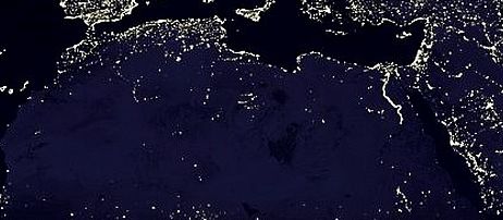
Africa at Night
Flashlight Use
PV Electrification
Martin Burian
Christof Arens
Lukas Hermwille
Hamburg, November 2012
Table of Contents
Abreviations .............................................................................................................................................. 3!
1! Introduction....................................................................................................................................... 5!
2! Methodology ..................................................................................................................................... 7!
3! SBL For Rural Electrification ........................................................................................................... 9!
  3.1!     Evaluating the Existing AMS I.L Defaults .............................................................................. 9!
  3.2!     Standardization of Rural Electrification Defaults for Ethiopia .............................................. 12!
     3.2.1! Household Lighting Baseline Emission Factor ................................................................. 12!
     3.2.2! Baseline Emission Factors of other HH Appliances ......................................................... 16!
     3.2.3! Baseline Emission Factors of other Consumers ................................................................ 20!
  3.3!     Comparing Default Emissions Factors with Standardized Factors........................................ 21!
4! Economic Evaluation of Carbon Revenues .................................................................................... 23!
5! Evaluation of Environmental Integrity ........................................................................................... 26!
6! SBL Implications On National MRV Systems ............................................................................... 30!
7! The Use of SBLs for New Market Mechanisms ............................................................................. 32!
8! Conclusions..................................................................................................................................... 34!
References ............................................................................................................................................... 36!
Annex I: Electricity Acess in Africa ....................................................................................................... 41!
Annex II: EF and Baseline Emissions based on AMS I.L ...................................................................... 42!
Annex III: Ethiopian Electricity Consumption in a Global Context ....................................................... 43!
Annex IV: Non-Annex I Grid Emission Factor ...................................................................................... 44!
Annex V: Load Duration Curves from Selected African Countries ....................................................... 47!
Annex VI: Investment Costs in African CDM PV Projects .................................................................... 50!
Annex VII: for Rural Electrification Programme Costs .......................................................................... 51!

                                                           SBLs in SSA and their Implications on MRV !                                                     1!
List of Tables
Table 1: Current Status of SBLs submitted to UNFCCC 6
Table 2: Default Factors of AMS I.L 10
Table 3: Efficiencies of Different Lighting Technologies 14
Table 4: Pressure Lamp Emission Factor at MSL 15
Table 5: Default Emission Factors for Diesel Generators 17
Table 6: Determination of the Average to Peak-Demand Ratio 19
Table 7: Technical Transmission Losses 19
Table 8: Determination of Installed Capacity 19
Table 9: Comparison of Default and Standardized Emission Factors 21
Table 10: Rural Electrification Program Costs, CDM Transaction Costs and Carbon Revenues 24
Table 11: Electricity Access in 2009 - Africa 41
Table 12: Electricity Consumption in Ethiopia in a Global Context 43
Table 13: IGES Grid Emission Factor Data 44
Table 14: Determination of the Average- to Peak-Demand Ratio 47
Table 15: Investment Costs in African CDM PV Projects 50
Table 16: Calculation of the Capital Costs for Rural Electrification 51
Table 17: Rural Electrification Program Costs, CDM Transaction Costs and Carbon Revenues 52
!List of Figures
Figure 1: Share of Baseline Emissions for 0.5MWh EC 11
Figure 2: Development of Electricity Consumption in Ethiopia 16
Figure 3: Rural HH Size in the Developing World 17
Figure 4: Figure 4: Comparison of Default- and Standardized EFs 22
Figure 5: Comparing Default and Standardized Baseline Emissions 22
Figure 6: Emission Factors and Baseline Emissions based on AMS I.L 42
Figure 7: Botswana Load Duration Curve 48
Figure 8: Lesotho Load Duration Curve 48
Figure 9: Mozambique Load Duration Curve 48
Figure 10: RSA Load Duration Curve 48
Figure 11: Swaziland Load Duration Curve 49
Figure 12: Tanzania Load Duration Curve 49
Figure 13: Zambia Load Duration Curve 49
Figure 14: Zimbabwe Load Duration Curve 49
SBLs in SSA and their Implications on MRV ! 2!ABREVIATIONS
AMS Approved SSC Methodology
BMU German Federal Ministry for the Environment, Nature Conservation and Nuclear Safety
CAR Corrective Action Requests
CDM Clean Development Mechanism
CDM EB CDM Executive Board
CER Certified Emission Reduction
CFLs Compact Fluorescent Lamps
CL Clarification Request
CM Combined Margin
CMP Conference of the Parties serving as Meeting of the Parties to the UNFCCC
DNA Designated National Authority
DOE Designated Operational Entity
EC Electricity Consumption
EF Emission Factor
GEF Grid Emission Factor
Gg Giga gram
GHG Greenhouse Gas
HH Household
IEA International Energy Agency
IPCC Intergovernmental Panel on Climate Change
kW kilo Watt (installed capacity)
kWh kilo Watt hour
LDC Least Developed Countries
LF Load Factor
lmn Lumen
lmn h Lumen hours
MSL Minimum Service Level
MW Mega Watt (installed capacity)
MWh Mega Watt hours
MRV Monitoring Reporting and Verification
NAMA National Appropriate Mitigation Actions
NCV Net Caloric Value
NIR National Inventory Report
NM New Methodology submitted to the UNFCCC
NMM New Market Mechanism
PoA Programme of Activities
PV Photovoltaic
SBLs in SSA and their Implications on MRV ! 3!ODA Official Development Assistance
QA/QC Quality Assurance/Quality Control procedures
RSA Republic of South Africa
SBL Standardized Baseline
SD Suppressed Demand
SOP Standard Operating Procedures
SSA Sub-Saharan Africa
SSC Small Scale
SSC WG Small Scale Working Group
UBA German Federal Environment Agency
UNFCCC Unite Nations Framework Convention on Climate Change
USD US Dollar
W Watt
SBLs in SSA and their Implications on MRV ! 4!1 INTRODUCTION
This study was commissioned by the German Federal Environment Agency (UBA). It complements
the study ‘Strategies for the Development of Carbon Markets in African Least Developed Countries,
commissioned by the German Federal Ministry for the Environment, Nature Conservation and Nuclear
Safety (BMU) and implemented by Perspectives GmbH.
The unequal distribution of the Clean Development Mechanism (CDM) is considered as major
shortcoming. The Conference of the Parties (COP) of the UNFCCC notes ‘equitable geographic
distribution of clean development mechanism among project activities at regional and sub regional
levels’ (Decision 17/CP.7, Marrakech Accords). Already in 2008, Mr. Rajesh Kumar Sethi, former
head of the CDM Executive Board, notes in the context of UNFCCC’s press release on the occasion of
the registration of the 1,000th CDM project: ‘The CDM is operating in close to 50 countries, and is
approaching its thousandth registered project with 128 million CERs already issued. Everyone
involved can take some pride in those states, but until the potential of the mechanism is realized in the
lesser developed countries, especially in Africa, we cannot rest’ (UNFCCC, 2008). Ever since much
time has passed and still the uptake of the CDM in Africa and other underrepresented regions is fairly
limited. Currently 247 CDM projects are registered in Africa, out of a total of 5,133.
The development of Standardized Baselines (SBL) may support the Least Developed Countries in up-
scaling their mitigation activities under the CDM. This may hold true as SBL offers the opportunity to
include Suppressed Demand in existing methodologies.
Since 2009, the UNFCCC Secretariat engages in putting SBL into operation. The Copenhagen Accords
decided that the Subsidiary Board for Technical Advice to the UNFCCC shall develop modalities and
procedures for Standardized Baselines. One year later, the COP in Cancun requested the CDM
Executive Board to develop Standardized Baselines which are defined as ‘a baseline established for a
party or a group of parties to facilitate the calculation of emission reductions and removals and/or the
determination of additionality for [CDM] project activities, while providing assistance for assuring
environmental integrity (Decision 3/CMP.6).
In the meantime the CDM EB provided a range of Guidelines and Procedures for SBL development
and the consideration of Suppressed Demand. And as of today, the first SBLs have been developed and
are submitted to the Secretariat for review and approval. The below table provides an overview on the
current SBL submissions.
SBLs in SSA and their Implications on MRV ! 5!Table 1: Current Status of SBLs submitted to UNFCCC
"#$#%#&'#! (%)*)+,-! ./01233#4!05!6!)&! 7/%%#&3!.3,3/+! 8,+3!9*4,3#!
F&232,-!,++#++;
(%)*)+#4!&#>!+3,&4,%42?#4! G,&,!)&!
0#@,-$!)$!:)3+>,&,P!Q"7P!
.3,&4,%42?#4!0,+#-2&#!)&!N%24! F&232,-!,++#++;
D)?,102R/#P!S,1202,P!
(.:;#!6!E=!M/B!
E2 METHODOLOGY
Chapter 3 investigates the potential of Standardized Baseline for rural electrification in Ethiopia.
Section 3.1 explores the existing default baseline emission factors provided by the applicable method-
ology. The following sources of information were used:
! Approved Small Scale (SSC) Methodology (AMS) IL, Electrification of Rural Communities
Using Renewable Energy, Version 01, CDM EB66.
! PÖYRY, 2011, Justification Document for Proposed New Baseline Methodology for Electrifi-
cation of Rural Communities, Final Report. Section 3.2 proposes own standardized baseline
emission factors. For this work, it was important to evaluate in detail the development steps of
the applicable methodology. As the AMS I.L, as approved by the CDM Executive Board
(CDM EB) at the Board’s 66th meeting, and the Justification Document show substantial dif-
ferences for the respective default Emission Factors (EF), we conducted a conference call with
the Methodology Panel of the UNFCCC Secretariat. The conference call was held at the 28th
September 2012.
The steps for standardization, developed in Section 3.2 strongly build on the current CDM rules and
requirements related to Standardized Baselines and Suppressed Demand (SD):
! Decision 3/CMP.6, §44-52;
! Guidelines for the Establishment of Sector-Specific Standardized Baselines, Version 2 ap-
proved at EB65, Annex 23.
! Procedure for Submission and Consideration of Standardized Baselines, Version2, EB68,
Annex 32).
! Guidelines for Quality Assurance and Quality Control of Data used in the Establishment of
Standardized Baselines, Version 1, EB66, Annex 49
! Guidelines for the Consideration of Suppressed Demand in CDM Methodologies (EB62, An-
nex 6).
The standardization of EFs requires detailed country specific data for the use of baseline technologies.
Lighting Africa1, an initiative by a World Bank/IFC initiative, promotes efficient lighting technologies
in selected African countries, including Ethiopia. For this purpose, Lighting Africa conducted
extensive baseline studies in Ethiopia on existing lighting technologies an off-grid energy appliances.
The related data were used for defining a Minimum Service Level as well as for identifying the
baseline technologies for lighting in Ethiopia.
1
Lighting Africa is a joint IFC and World Bank program that works towards improving access to better lighting in
areas not yet connected to the electricity grid. It aims at catalysing the development of sustainable markets for
affordable, modern off-grid lighting solutions for low-income households. General information on the initiative
may be found under: www.lightingafrica.org
SBLs in SSA and their Implications on MRV ! 7!Chapter 4 evaluates the economic impact of a CDM Programme of Activities on a rural electrification
program in Ethiopia. Based on the findings of Chapter 3, the carbon revenues were assessed and
compared to the overall capital costs for financing renewable, rural electrification activities.
Chapter 5 evaluates the environmental integrity of SBLs under the consideration of suppressed
demand. This analysis evaluates the existing guidelines and procedures with respect to their provisions
for quality assurance and quality control. The evaluation is supported by the Consultant’s own
experience in developing the first SBL to be considered by the CDM EB.
Chapter 6 assesses the synergies between SBLs and national Monitoring, Reporting, and Verification
systems. This is done by comparing the capacity needs of national reporting with those required for
SBL establishment.
Chapter 7 explores the use of SBLs for New Market Mechanisms. The need of New Market Mecha-
nisms to have a transparent and commonly accepted baseline is evaluated. This need is contrasted with
the current accounting of national greenhouse gas inventories. Finally the New Market Mechanism’s
need for baseline setting is compared to the approach for SBL development.
SBLs in SSA and their Implications on MRV ! 8!3 SBL FOR RURAL ELECTRIFICATION
This chapter is driven by the question, whether standardization of default emission factors for rural
electrification may provide additional benefits, compared to the -already significant- default emission
factors provided in methodology AMS I.L.
Hence, this section covers two technical steps for evaluating the benefits of a possible standardization
of AMS I.L: First, the existing emission factors are evaluated (Chapter 3.1) . This is done based on the
approved methodology. Second, Chapter 3.2 explores options for the development of alternative
emission factors for rural electrification.
3.1 Evaluating the Existing AMS I.L Defaults
Scope of AMS I.L. At its 66th meeting, the CDM Executive Board approved the Small Scale method-
ology ‘AMS I.L – Electrification of Rural Communities Using Renewable Energy2’. AMS I.L allows
for generating Certified Emission Reductions (CERs) for renewable CDM projects which electrify
rural communities that have no access to any electricity distribution system prior to project implemen-
tation. The methodology was proposed by Pöyry Management Consulting with support from the UK
Department for International Development and the World Bank. It underwent significant changes
based on the input from the Small Scale Working Group and the UNFCCC Secretariat before approval.
The methodology applies an innovative approach in two regards:
! First, the methodology is strongly based on the concept of suppressed demand. The baseline
scenario is based on a minimum service level, i.e. the energy level required to meet basic hu-
man needs. This is in sharp contrast to common baseline scenario approaches which are based
on historic data.
! Second, AMS I.L offers a highly standardized approach. It proposes the use of three default
emission factors which can be applied without further evidence or reference documents. In this
regard, AMS I.L is in line with the Secretariat’s efforts to increase the standardization of the
CDM (and hence its applicability).
The result is a fairly simple methodological concept which is easily applicable in the context of Least
Developed Countries which are often hampered by data availability.
Evaluation of Default Emission Factors. Subsequently, the methodology AMS I.L is evaluated in
more detail. It is based on three default Emission Factors (EF) which are linked to different energy
services. The exact energy services and the emissions related to them are not explicitly stated in AMS
I.L; however, they are well documented in the background documents (Pöyry 2011 and SSC Working
Group 34). The default Emissions Factors are as follows:
2
Please refer to AMS I.L, Version1.
SBLs in SSA and their Implications on MRV ! 9!! For the first 55 kWh consumed by a household (HH), an EF of 6.8 tCO2/MWh is applicable
(AMS I.L, Version 1, §9.a). This EF is based on electricity consumption for household lighting
services (Pöyry, 2011, p11f).
! It is assumed that further electricity consumed per HH (up to 250kWh per year) is used for
other household appliances. For this electricity consumption, a default EF of 1.3 tCO2/MWh is
applicable (AMS I.L, Version 1, §9.b). This EF considers emissions related to the electricity
consumption of other household appliances, such as TV, radio, fans, cell phone chargers etc. It
is further assumed that the electricity consumption of other household appliances is met by a
mini-grid served by a diesel generator (SCC WG34, §5.iii).
This is in contrast with Pöyry’s initial proposal of an EF of 3.4 tCO2/MWh. This is based on
the default EF of a small scale diesel generator (EF: 2.4tCO2/MWh) and a battery loading effi-
ciency of 75% (Pöyry, 2011, p15). Thereby Pöyry referred to the default EF of a diesel genera-
tor with an installed capacity below 15 kW and a load factor of 25% or less (AMS I.F, §13).
! Finally, for any electricity consumption above 250 kWh/yr by households or other electricity
consumers (e.g. SMEs), a default EF of 1 tCO2/MWh is applicable (AMS I.L §9.c). This emis-
sion factor is based on the default EF for a diesel generator with an installed capacity of 135-
200 kW and a load factor of 50% (cp. SSC WG34, §5.iv).
Model Calculation for One Household. Based on these default emission factors, this section presents
a model calculation for a single household. This calculation determines the volume of CERs that can be
generated by a rural electrification project, based on renewable energy. The calculation is based on the
assumption that the household consumes 500 kWh/yr. This value was chosen to allow for the analysis
of the different default values of the methodology as presented in Table 2 below, despite the fact that
actual average household consumption is still lower in Ethiopia (see Annex III: Ethiopian Electricity
Consumption in a Global Context). However, this assumption is still in line with values of electricity
consumption in rural households in other developing countries ranging from 228 to 768 kWh/yr/HH as
stated in Pöyry, 2011, Table 1, p10.
Table 2: Default Factors of AMS I.L
M''/1/-,3#4!I-#'3%2'235!
:,+#-2&#!I12++2)&! I12++2)&!W,'3)%!! :,+#-2&#!I12++2)&+!!
7)&+/1*32)&!!
.)/%'#! X2&!37\E6DY@[! X2&!37\E65%[!
X2&!HY@!*#%!ZZ65%[!
ZZ!82B@32&B! !Figure 1: Share of Baseline Emissions for 0.5MWh EC As can be seen from the table
above, the methodological ap-
proach laid out by AMS I.L results
in 0.374 tCO2 for the first
55kWh/HH/yr.
The electricity consumption (EC)
from 56-250 kWh/HH/yr accounts
for 0.254 tCO2.
Based on above assumption of 500
kWh/HH, the consumption from
251-500 kWh/HH/yr amounts to
0.250 tCO2. As a result, a rural
electrification program may gene-
rate 0.878 CERs per HH and year.
The figure to the left shows the
Source: Calculated based on AMS I.L, Version 1. contribution of the specific EFs to
the overall baseline emissions of
one household: Despite making up for only 11% of the total household electricity consumption, the
first 55kWh account for 43% of the household’s baseline emissions. The categories 56-250 and 251-
500 kWh make up for 29% and 28% respectively. Annex II provides a figure comparing the emission
factors with their related baseline emissions.
Context Evaluation. In a concluding step, the above findings are evaluated in a broader context. The
above determined 0.878 CERs/HH sum up to 1.756 CERs/MWh. As reference the following other
baseline emission factors may be used:
! Annex IV provides data on all Grid Emission Factors (GEF) which have been submitted to
UNFCCC up to date. This data was aggregated by the Institute for Global Environmental Stud-
ies (2012). It shows that the average Combined Margin (CM) amounts to 0.824 tCO2/MWh.
! Default emission factors for larger diesel sets range from 0.8 to 1.3 tCO2/MWh (AMS I.F,
Version 2, §13).
Comparing baseline emissions determined under AMS I.L (1.756 tCO2/MWh) with average GEF, the
AMS I.L baseline emissions amount to 213% of the average GEF value. The baseline emissions are
also considerably higher than the defaults of larger diesel generators. Such high baseline emissions are
well justified: The selection of kerosene pressure lamps as baseline technology for lighting, for
example, demonstrates the conservativeness of the approach. Despite the fact that this type of lamp is
not (yet) commonly used to provide lighting, it was chosen instead of the roughly 10 times less
efficient but widely used kerosene wick lamps. Furthermore, off-grid demand is usually covered by
small diesel generators, which have usually much higher emission factors than the national grid. Last
not least, the AMS I.L baseline emissions already include suppressed demand which is also not
included in the GEF value.
SBLs in SSA and their Implications on MRV ! 11!Conclusion. AMS I.L, Version 1, offers a high degree of standardization. Moreover, the concept
of Suppressed Demand, defined as a minimum energy consumption level, leads to substantial
CER volumes per unit renewable energy.
3.2 Standardization of Rural Electrification Defaults
for Ethiopia
Chapter 3.1 concludes that AMS I.L features a high degree of standardization combined with substan-
tial emission factors based on Suppressed Demand. Against this background, this Chapter is driven by
the question, whether the further standardization of EFs allows to exceed the default EFs provided by
AMS I.L. The subsequent approach for standardization is based on an enforced emphasis on sup-
pressed demand for lighting technologies as well as the investigation of load factors for off-grid diesel
generators. The sketch for the standardized baseline is developed for the following regional scope:
! The concept for the standardized baseline is development for the Federal Democratic Republic
of Ethiopia. The country was chosen by the Federal Environment Agency and the German
Federal Ministry for the Environment, Nature Conservation and Nuclear Safety (BMU).
! If national data was not available, regional data covering Sub-Saharan Africa (SSA) or from
single SSA countries was used.
Subsequently, we investigate options for increasing the baseline emissions through standardization
following the Pöyry’s stepwise approach, starting with HH lighting, other HH appliance and conclud-
ing with baseline emissions of other consumers.
3.2.1 Household Lighting Baseline Emission Factor
Defining a Minimum Service Level. Following the methodology justification document (Pöyry 2011,
p12ff), in a first step a benchmark for a Minimum Service Level (MSL, i.e. in terms of lighting
services) is established. The original approach proposed by the methodology justification document
was not followed due to a lack of detailed data (SSC WG34, §3.ii). This issue is picked up in below
sections based on detailed data sets for Ethiopia.
Pöyry (2011, p13) established a satisfied demand level of two Compact Fluorescent Lamps (CFLs)
with a power rating of 15W. This was done in the context of the IEA’s definition of a minimum energy
service level (IEA, 2010, p19). Pöyry states (2011, p13) that ‘the lighting levels of two 15W CFLs is
approximately 1,700 -1,800 lumens from the lamp’. Mills (2003, p11) documents an output of 873
Lumen for a 15W CFL. Consequently, the satisfied demand level is determined at 1,746 Lumen per
household.
Conclusion. MSL of lighting was defined at 1,746 lumen per household (AMS I.L.)
SBLs in SSA and their Implications on MRV ! 12!Determining the Baseline Technology. The Executive Board established Guidelines on the Consider-
ation of Suppressed Demand in CDM Methodologies (CDM EB68, Annex 2). We subsequently follow
these to strengthen the applicability of SD. CDM EB68, Annex 2, §13 proposes four steps to identify
the appropriate baseline technology under a suppressed demand scenario. These steps are applied based
on a detailed market analysis for lighting appliances, conducted by Lighting Africa Lighting Africa,
2008. One of Lighting Africa’s focus countries is Ethiopia the current lighting practices of which are
analyzed in depth, covering lighting hours, number of lighting devices per household, current lighting
technologies etc. The sample size for Ethiopia was 1006.
! Step 1: Identification of Alternative Technologies. In a first step, the available lighting tech-
nologies are screened. These are:
o Simple kerosene lamp with no cover;
o Kerosene lamp with cover;
o Pressurized Kerosene lamp;
o Firelight, and
o Candle.
! Step 2: Compliance with Local Regulations. All technologies are in compliance with local
regulations.
! Step 3: Rank Technologies by Decreasing Efficiency. In this step, efficiency is defined as
lumen hours (lmn h) by liter of fuel consumption. The efficiencies of different technologies are
presented in the table below. The following methodological approach is applied:
o Market penetration data was taken from Lighting Africa (2008, p79)3.
o Fuel consumption and lumen output-data was taken from Mills (2003) who tested var-
ious technologies.
3
Please note: The survey covers flashlights (8.93%). Lighting Africa (2011, p17) states ‘that the low usage of flashlights …
reflects the fact that flashlights are mainly used to light the way to the toilet outside or as a backup light and not as a main
device to light the living room’. Consequently, flashlights were not included in step 1 above nor considered here. Moreo-
ver, the survey showed that 8% of the population used 'Light bulb in a socket'. As the SBL focuses on off-grid electrifica-
tion, this baseline technology was removed. Finally, please note that he survey collected information on the ‘lighting
technology applied last night’. There were a few persons using more than one technology. Hence survey results were
normalized to 100%.
SBLs in SSA and their Implications on MRV ! 13!Table 3: Efficiencies of Different Lighting Technologies
8,1*!>23@!
(%#++/%#! 8,1*!>23@!
O5*#! .21*-#!Y2'H!,&4! 7,&4-#+! W2%#-2B@3!
8,1*! 7)`#%!
S)!7)`#%!
D,%H#3!(#%,32)&!2&!I3@2)*2,!Determination of the Baseline Emission Factor for Table 4: Pressure Lamp Emission
Lighting. Moreover, as the baseline technology is identified, Factor at MSL
it is possible to determine the baseline emission factor. The
following methodological steps are applied: F3#1! _,-/#!
! The Tier 1 Net Caloric Value (NCV) of Kerosene was I$$2'2#&'5!
=CPJJG!
taken from the IPCC Guidelines for National Greenhouse X2&!-1&!@6-[!
Gas Inventories (IPCC, 2006, page 1.18). S7_!
JGL^!
! The Tier 1 EF for Kerosene was taken from the 2006 X2&!OK6NB[!
IPCC Guidelines for National Greenhouse Gas Invento- IW!!
U=Lb3.2.2 Baseline Emission Factors of other HH Appliances
Electricity Consumption in Ethiopia. Ethiopia is characterized by low electricity consumption
patterns per capita. The actual consumption in 2009 amounts to 45.76 kWh/yr and person (IEA
Statistics, 2011). Annex III puts the electricity consumption in Ethiopia in a global context: It shows
that the electricity consumption per capita (data from 2008) is the lowest from all 30 countries which
are compared.
This data was extrapolated at household level. Ethiopia’s Central Statistical Agency (2008) reports an
average rural household size of 4.9 persons. The below figure illustrates the increase of electricity
consumption per household (based on a fixed household size of 4.9 persons). The IEA defines an
‘Universal Electricity Access Case’ (2009, p.132): ‘Basic electricity consumption in rural areas is
assumed to be 50 kWh per person per year’.
Considering this electricity consumption volume per person and the rural household size, the minimum
electricity consumption level amounts to 245 kWh per HH, per year. This is value is illustrated as the
blue line ‘IEA Universal Electricity Access’ in below graph. The analysis shows that the average
electricity consumption level in Ethiopia is below the minimum value defined by the IEA.
Figure 2: Development of Electricity Consumption in Ethiopia
Source: Based on data from A) IEA Statistics and B) Central Statistical Agency of Ethiopia, 2008
Minimum Service Level for Household Energy Consumption. Against the above context, an MSL
for electricity consumption at household level is elaborated. The IEA (2010, p19) defines the minimum
electricity consumption level for a rural household at 250kWh/yr. This value was proposed by Pöyry
(2011, p10) and adopted in AMS I.L (§9.b). In 2009, the IEA (page 132) defined the ‘Universal
Electricity Access Case’ which specifies a minimum electricity consumption level of 50 kWh per
person. Both definitions are consistent, if an average rural household size of five persons is assumed.
SBLs in SSA and their Implications on MRV ! 16!This assumption seems
Figure 3: Rural HH Size in the Developing World
reasonable as the average HH
level in the developing world
ranges in this size. John
Bongaarts, Vice President of the
‘Population Council’, evaluated
the average size of rural HH
(2001). His findings show values
ranging from 5.0 (Latin
America) to 6.1 persons (Near
East and North Africa).
However, for the specific case of
Ethiopia, the average, rural
household size amounts to 4.9
persons (CSA, 2008). Based on
CSA’s lower value and based on
IEA’s 2009 definition, the
Source: Based on data from Bongaarts (2001, p25) and Central minimum service level for
Statistical Agency of Ethiopia (2008).
electricity consumption at rural
household level in Ethiopia is defined at 245 kWh per year, per HH, which is considered as conserva-
tive.
Determination of the Baseline Emission Factor for HH EC. In a next step, the emission factor for
household electricity consumption is evaluated. For electricity consumption at HH level (i.e. up to 250
kWh) AMS I.L determines a default EF of 1.3 tCO2/MWh (AMS I.L, Version 1, §9.b). It is assumed
that this electricity demand is met by a mini-grid served by a diesel generator (SCC WG 34, §5.iii)
with an installed capacity in the range of 15-30 kW, with a load factor of 50%. The default emission
factors for diesel generators are provided in table below.
Table 5: Default Emission Factors for Diesel Generators
8),4!W,'3)%!
F&+3,--#4!7,*,'235! E]a! ]generators in rural areas in Ethiopia. This study therefore adopts the size as determined by SSC WG34,
§5.iii.
Second, the typical load factor for diesel
Box: What is a Load Factor?
generators in Sub-Saharan Africa is assessed. As
shown by the table above, diesel generators The load factor (LF) determines the average
operate more efficiently at full load. Hence the utilization rate of a power generation unit. It is
emissions per unit of electricity produced usually calculated on an annual basis by comparing
decrease by an increasing load factor. the maximum output (i.e. at full load) by the actual
It is common understanding that any off-power output.
generation system needs to accommodate the To give a practical example: A hydropower plant
peak demand. Consequently, off-grid systems features an installed capacity of 1 MW. In a given
are typically oversized and operate at low load year, the electricity output amounts to 2,628 MWh.
factors. Contreras (2008) evaluated dimension- The maximum output is determined by 1 MW x
ing parameters for rural electrification by diesel 24h x 365d equaling 8,760 MWh. The LF is
generators in Sub-Saharan Africa (i.e. in determined by dividing the actual output by the
Senegal). maximum output which results in a load factor of
In order to adequately dimension the diesel 30%.
generator for a mini grid, the data on the peak
demand and the transport loss factor are !"#$%&!!"#$"!!
!!! ! ! !"#$%&%!!"#$"# (1)
required. Based on these, the installed capacity
Whereas:
of diesel generators may be determined by the
LFn: Load Factor in %
following formula (Contreras, 2008):
Actual Outputn: Actual electricity generated
!!! !!"#$ in year n, in MWh
!!"# !"# ! !!! (2) Maximum Output: Maximum electricity output
!"""!!!!! !!
of the power plant at full
Whereas load in any year, in MWh
Peng: Engine capacity in kVA
Ppeak: Peak demand in W
f 1: Transport loss factor
In a next step, the relation of average demand to the peak demand is evaluated. Here, peak demand is
defined in a narrow sense, i.e. as the highest electricity demand in one year, which is usually deter-
mined based on hourly- or half-hourly data.
A literature review was conducted to identify appropriate default factors. IEA (2012, p14) notes: ‘The
power balance challenge for mini-grids in remote communities is increased by load profiles which are
often highly variable, with the peak as high as 5 to 10 times the average load’. Elamari et al. come to
the identical conclusion (2011, p842): ‘This is not an easy task considering that remote communities
are characterized by highly variable loads with peak load as high as 5 to 10 times the average load.’
Pelland et al. (2011, p2) report on an average to peak ratio of 259% based on a detailed monitoring of
one single hybrid system. Moreover Prof. Luis Vargas Díaz from the Universidad de Chile, Facultad de
Ingeneria Electrica provided data on a Diesel mini grid in the North of Chile, Huatacondo, where the
average to peak ratio amounts to 222%.
SBLs in SSA and their Implications on MRV ! 18!Finally, the load data from eight Sub-
Table 6: Determination of the Average to Peak-
Saharan African countries was evaluated. On
Demand Ratio
the one hand, this data is a sound data
.)/%'#! _,-/#! source, as it is based on full time monitoring
FIMP!ENote on the Application of Car Batteries and Related Efficiencies. As discussed above, Pöyry
considered the use of car batteries which are charged at rural mini-grid diesel systems. Hence, Pöyry
(2011, p15) divided the related default emission factor by the charging efficiency (i.e. 75%) thereby
increasing the emission factor by 25%. This approach was rejected by the SSC WG34, §5.1.
The use of car batteries was evaluated for Ethiopia, but was found to be inappropriate. Lighting Africa
(2008, p70) found that only 1% of traders used car batteries (out of a sample of 400 shops). It is
assumed that the penetration ratio at household level is lower. Hence the related efficiency losses were
not considered in for the standardization of baseline EFs.
Conclusion. The baseline emission factor for household appliances is determined at 1.9
tCO2/MWh.
3.2.3 Baseline Emission Factors of other Consumers
For electricity provided to other consumers (i.e. defined as electricity above 250 kWh/yr supplied to a
single consumer), AMS I.L determines a standard EF of 1.0 tCO2/MWh (AMS I.L, §9.c). This is
related to the emission factor of mini-diesel grids with an installed capacity of 35- 135 kW and a load
factor of 50%.
As elaborated in section 3.2.2, off-grid systems are characterized by low load factors. In analogy to the
above, a load factor of 25% seems appropriate. Consequently, a higher emission factor is applied. The
corresponding EF amounts to 1.3 tCO2/MWh (please refer to Table 5 above).
Conclusion. The baseline emission factor for ‘other consumers’ is determined at 1.3 tCO2/MWh.
SBLs in SSA and their Implications on MRV ! 20!3.3 Comparing Default Emissions Factors with
Standardized Factors
Chapter 3.1 evaluates the existing EFs as approved by AMS I.L, §9, while chapter 3.2 discusses
whether it is appropriate to propose higher EFs for rural electrification activities in Ethiopia. Two
findings lead to the proposal of higher emission factors:
! Strong emphasis on suppressed demand combined with reliable data on current lighting tech-
nologies and related emissions lead to the standardization of the EF for household lighting. A
standardized EF of 9.1 tCO2/MWh is proposed for Ethiopia. Compared to AMS I.L, this means
an increase of the EF by 25.3%, resulting into an increment of 0.13 CERs per HH.
! Second, the choices of load factors are reviewed. It is found that mini-grid diesel generators are
generally operating at a lower load factor than assumed by AMS I.L. As a consequence, the
EFs for ‘Other Household Appliances’ and ‘Other Consumers’ were increased to 1,9
tCO2/MWh and 1.3 tCO2/MWh respectively. This results in an increase of 0.28 CERs per HH
and year (assuming that one HH consumes 0.5 MWh/yr).
These findings are presented in below table:
Table 9: Comparison of Default and Standardized Emission Factors
Q#$,/-3!I12++2)&!W,'3)%+!)$!MD.!FL8! .3,&4,%42?#4!I12++2)&!W,'3)%+!
!
:,+#-2&#! :,+#-2&#! :,+#-2&#!
IW!! IW!!
I12++2)&! IN!*#%!ZZ65%! I12++2)&+! I12++2)&+!
X37\E6DY@[! X37\E6DY@[!
.)/%'#! X37\E65%[! X37\E65%[!
ZZ!82B@32&B!Figure 4: Figure 4: Comparison of Default- and Standardized EFs
The graph above illustrates the comparison of emission factors (i.e. tCO2/MWh) for different electricity
consumption categories.
Figure 5: Comparing Default and Standardized Baseline Emissions
The graph above illustrates the comparison of baseline emission factors per electricity consumption
category and the overall total per HH on an annual level. The bars at the right (blue for the standard-
ized approach, red for the default EFs, as specified in AMS I.L) present the aggregated baseline
emissions over all three energy consumption categories.
This result demonstrates that the standardization approach developed in Chapter 3.2 allows to
significantly increase the baseline emission factor. This leads to a significant increase of CERs per
household to be generated by a rural electrification program.
SBLs in SSA and their Implications on MRV ! 22!4 ECONOMIC EVALUATION OF CARBON
REVENUES
This chapter evaluates the potential carbon revenues for a rural electrification program in Ethiopia. For
this purpose, a general cost structure for a rural electrification support program was established. The
impact of carbon revenues was assessed against this structure. The following methodology and
assumption/input data was applied:
! The average investment costs for PV systems in Africa is determined by calculating the aver-
age investments in 1 kW installed capacity in African CDM projects. The average investment
costs amount to 3,573 USD/kW, the raw data is provided in Annex VI.
! An exchange rate of 1! : 0.77 USD is applied (XE, 2012) for determining average investment
costs in !. This equals an investment volume of 2.75 mio !/MW and 6.88 mio ! per year (see
below).
! It is assumed that a rural electrification program in Ethiopia would have an average outreach of
2.5 MW/yr for 10 years. It is assumed that the Rural Electrification Executive Secretariat sup-
ports private companies in the implementation of off-grid activities, but the actual electricity
generation devices are operated and owned by a private entity.
! Moreover, it is assumed that the private entity invests 20% of equity and receives a loan in the
amount of 80% of the investment volume. Hence, the annual loan volume for the whole pro-
gramme would amount to 5.51 mio !/yr. It is further assumed that such a loan is paid back
within 10 years.
! Any electrification project would have to pay interest in the amount of 14.5% p.a. The interest
rate was taken from the benchmark for energy investments in Ethiopia, as provided by CDM
EB62 (Annex 2, Appendix, § 8).
Findings. Based on above considerations, the capital costs for rural electrification activities are
determined. The actual data is provided in Annex VII, Table 16. The discounted capital costs for the
total electrification program (25 MW installed capacity, implemented over 10 years) amount to 13.36
mio !.
In a next step, the costs of the rural electrification support program, CDM transaction costs and the
related carbon revenues are estimated.
! It is assumed that the personnel and office cost of a rural electrification support program
amount to 100,000 !/yr (expert estimate for 2-3 persons, office- and vehicle costs).
! The CDM transaction costs are estimated as follows: CDM Programme of Activity (PoA)
development costs amount to 50,000!, Validation and Registration costs amount to 35,000!.
The annual verification costs amount to 25,000! (expert estimate).
! Moreover it assumed that the PoA operates for a crediting period of 28 years (4 times 7 year
crediting periods). It shall be noted that the climate finance for Least Development Countries is
not determined for that time period. Still, the climate finance contribution from e.g. year 2040
to the discounted revenues is very limited (e.g. 21,985! for 2040), which is due to Ethiopia’s
high interest/discount rate.
SBLs in SSA and their Implications on MRV ! 23!! Efficiency ratios for solar PV in Africa range between 15% (international default value of
AMS-I.L) and 24% (average of values in CDM PV projects submitted to UNFCCC). For the
economic analysis it is assumed that the PV off-grid appliances operate at a efficiency ratio of
24%, thus referring to a value based on real-life projects.
! It is assumed that each HH consumes 250 kWh/yr, which is in line with Ethiopia’s current
average electricity consumption per HH (please refer to Figure 2, page 16).
! Based on the above-mentioned load factor and electricity generation per HH per year, 1 MW
installed capacity will generate 5,256 MWh/yr. This may supply 21,000 HH with renewable
electricity and would result in 18,322 CERs/yr.
Findings. Based on above considerations, the annual ‘Totals’ can be calculated. Subsequently, these
figures were discounted by above interest rate resulting in the ‘Annual Discounted Totals’. The actual
figures are presented below for the years 2013 to 2019. For all results (i.e. 2013 to 2040) please refer to
Annex VII, Table 17, page 52. The aggregated, discounted net revenues (i.e. over 28 years) amount to
3.35 mio !.
Table 10: Rural Electrification Program Costs, CDM Transaction Costs and Carbon Revenues
h#,%! EA=&$*?D#=&7(O@#!$)--)>2&B!')&'-/+2)&+!,%#!4%,>&V!
! 7/%%#&3-5P! 3@#! 7QD! 2+! ')&+24#%#4! ,+! ,&! /&'#%3,2&! $2&,&'2&B! +)/%'#L! O@#! 7I"! *%2'#!
4#`#-)*1#&3! 2+! +/0A#'3! 3)! +*#'/-,32)&+! )&! ,44232)&,-! 4#1,&4! $%)1! 3@#! I/%)*#,&!
9&2)&!,&4!,!-)&B;3#%1!'-21,3#!*)-2'5!$%,1#>)%H!2+!,0+#&3L!
! h#3! 0,+#4! )&! )/%! ',-'/-,32)&+! 3@#! ',%0)&! %#`#&/#+! ')/-4! 0#! ,! `2,0-#! $2&,&'2&B!
+)/%'#P! ')`#%2&B! 3@#! )*#%,32`#! ')+3+! )$! ,! %/%,-! #-#'3%2$2',32)&! *%)B%,1L! M$3#%! +/0;
3%,'32&B!)*#%,32`#!')+3+P!3@#!7QD!>)/-4!%#+/-3!2&!,BB%#B,3#4P!42+')/&3#4!!%#`#;
&/#+!2&!3@#!,1)/&3!)$!GLG]!12)!jL!!
! ./'@! $/&42&B! ')/-4! 0#! /+#4! #LBL! 3)! %#4/'#! 2&3#%#+3! %,3#! )$! ')1*,&2#+! #&B,B2&B! 2&!
%/%,-!#-#'3%2$2',32)&L!Z)>#`#%P!',%0)&!$2&,&'#!>2--!&)3!0#!+/$$2'2#&3!3)!')`#%!3@#!1,;
A)%235!)$!3@#!',*23,-!')+3+!6!2&3#%#+3!*,51#&3L!O@#!3)3,-!',*23,-!')+3+!,1)/&3!3)!=GLGC!
12)!jL!7,%0)&!$2&,&'#!,1)/&3+!3)!GLG]!12)L!jP!1,H2&B!/*!$)%!E]a!3@#!',*23,-!')+3+!
,--)>2&B!3)!+/0+3,&32,--5!%#4/'#!3@#!2&3#%#+3!%,3#L!
SBLs in SSA and their Implications on MRV ! 25!5 EVALUATION OF ENVIRONMENTAL IN-
TEGRITY
This chapter briefly evaluates the environmental integrity of SBLs, i.e. the risk that the application of
an SBL leads to an overestimation of emission reductions. This may be the case if the CDM EB
approves an SBL featuring e.g. emission factors which are too high. The CDM EB provides three core
documents which are subsequently used for further evaluation:
! CDM EB68, Annex 32, Procedure for the Submission and Consideration of Standardized
Baselines, Version 2;
! CDM EB66, Annex 49, Guidelines for Quality Assurance and Quality Control of Data used in
the Establishment of Standardized Baselines, Version 1; and
! CDM EB65, Annex 23, Guidelines for the Establishment of Sector Specific Standardized
Baselines, Version 2.
Moreover, this evaluation is based on GFA’s own experience in developing the first SBL which was
submitted to the CDM EB for consideration (GEF for Southern African Power Pool). The environmen-
tal integrity is evaluated against the above-mentioned regulations.
In a first step, the data for SBL development has to be collected and compiled. The CDM EB defines
extensive and demanding Quality Assurance and Quality Control (QA/QC) procedures for data
collection. The collected data shall meet the following quality requirements: Relevance, Completeness,
Consistency, Currentness, Accuracy, Objectivity, Conservativeness, Security, Transparency and
Traceability (CDM EB66, Annex 49, §11.a-k). In the following, key qualities and related procedures
are discussed in detail:
! Completeness
For the compilation of the data for SBL development, the Designated National Authority
(DNA) shall include all relevant activity data (CDM EB66, Annex 49, §17). A conservative
approach for extrapolation of missing data is provided (CDM EB66, Annex 49, §18).
! Accuracy
The DNAs are encouraged to implement measures for avoiding errors. Sources of uncertainties
should be identified and reduced as far as practicable (CDM EB66, Annex 49, §19). If sam-
pling approaches are applied, the DNA should determine confidence intervals for the quantifi-
cation of conservative activity data (CDM EB66, Annex 49, §20).
! Transparency
If applicable, the DNA should invite stakeholders to provide comments on the SBL. The con-
sultation should be done in an open and transparent manner (CDM EB66, Annex 49, §21).
Second, in order to submit a SBL to the Secretariat, the DNA shall require an assessment report from a
Designated Operational Entity (DOE) ‘on the quality of the data collection, processing and compilation
to establish the proposed standardized baseline’ (CDM EB68, Annex 2, §7.b). The DOE shall be
accredited by the UNFCCC for the validation and verification of CDM Scopes (e.g. ‘energy industries
– renewable/ non-renewable sources’).
SBLs in SSA and their Implications on MRV ! 26!In the case of the SBL for the GEF in Sub-Saharan Africa, the contracted DOE assessed the SBL
similar to the validation process for a CDM project. The DOE drafted a validation protocol, issued
Corrective Action Requests (CAR) and Clarification Requests (CL) which were closed through the
amendment of the calculations and/or the SBL document. Once all CARs and CLs were closed, the
DOE issued the assessment report (similar to the final validation report).
Finally, once submitted, the Secretariat will engage its own SBL assessment procedures:
! Within 21 days of receipt, the Secretariat shall conduct an ‘initial assessment’ (specified in
CDM EB68, Annex 32, §11-13).
! Thereafter the Secretariat shall select two members of a panel or working group, who shall
‘independently assess the proposed standardized baseline’, draft a recommendation and inform
the CDM EB on the outcome. Afterwards, the CDM EB then will consider the SBL in its next
meeting (CDM EB68, Annex 32, §14-27).
The above procedures require substantial efforts to ensure completeness, accuracy and transparency of
standardization. Moreover, for many of the required sub-steps, the DNAs need to be actively involved
and leading the SBL validation- and approval processes. Finally, SBL-development and –validation
will require a highly specialized CDM expertise.
Working experience with DNAs in LDCs (cp, Burian et al. 2011 and Arens and Burian 2012) shows
that DNAs are frequently understaffed and the CDM responsible often has to assume a wider range of
responsibilities, i.e. the CDM being only one of several tasks. Hence Mersman and Arens conclude
(2012, p.12): ‘The [SBL] development process, as envisaged right now, lays a heavy burden on
countries' Designated National Authorities. Not only are they set as the main authorities in the
development of SBLs, and need to approve proposed SBLs that target their country, but they also have
the duty to control the quality of the data used for the proposal. As they often only have limited
financial and technical capacities, it is unlikely that DNAs will develop many SBLs under the current
conditions.’ It is concluded that a streamlined support process for SBL development may be key for a
broader uptake of SBLs in least developed countries.
Environmental Integrity in the Context of Suppressed Demand. SBLs may be based on the concept
of suppressed demand. This will lead to an SBL that overestimates the baseline emissions compared to
historical emissions. It implicitly anticipates future demand.
In this context, the CDM EB acknowledges the people’s right for a Minimum Service Level, applicable
to determine the baseline emissions under consideration of suppressed demand (CDM EB68, Annex 2),
which is per se a moral decision.
In the case of rural electrification, the minimum service level for electricity set out in the ‘Universal
Electricity Access Case’ (IEA, 2009, p.132). The baseline emissions are determined by the emissions
of the MSL in a conservative manner, as MSL baseline emissions shall be determined by the technolo-
gy which most efficiently achieves the MSL (CDM EB68, Annex 2, §13, Step 5).
Furthermore, the approach of suppressed demand is not exclusive to rural electrification projects.
Virtually all renewable energy projects revert to it. A wind farm constructed as a CDM project will not
demonstrate by how much emissions are being reduced in other power plants but emission reductions
are calculated simply compared to what would have happened in the absence of the CDM project
SBLs in SSA and their Implications on MRV ! 27!assuming that the hitherto suppressed demand would have been met by a baseline technology power
plant. In the case of rural electrification it is no different. The proposed methodology asks what
technology is necessary to provide a minimum service level and uses the emissions of this baseline
technology as basis for calculating emission reductions regardless of the extent of use of the baseline
technology.
The CDM’s purpose is to promote sustainable development in developing countries. The concept of
suppressed demand allows the CDM to assist in achieving the most basic development in a more
sustainable manner by leapfrogging unsustainable development stages. Environmental integrity is thus
ensured by sidelining conventional, unsustainable development at the earliest stage.
Update of SBLs. An inappropriate updating of SBLs may eventually compromise the environmental
integrity of the CDM: Assuming that the baseline emissions are determined by the SBL and the
real/actual emission trend of the sector decreases (e.g. the emission intensity of the cement sector
decreases as several cost effective and hence business as usual efficiency measures are implemented).
If the SBL would now have a validity of e.g. three years, whereas project-specific approach is
improved on an annual basis, then the application of the SBL would lead to an overestimation of
baseline emissions. Hence, in regard to environmental integrity the question is how likely a significant
decrease of emissions is within this timeframe.
The most recent version of the SBL Guidelines (CDM EB65, Annex 23) encloses an appendix which
suggests a validity of standardization for three years. CDM project development in practice also
operates with similar data validity. Many methodologies require the application of ‘the most recent
data available’ at validation (e.g. CDM EB63, Annex 19). Still data availability is often constrained
and data collection may be a time consuming and cost intensive process. Hence in 2012 numerous
CDM projects were registered which were based on data sets with vintage 2010. It may be concluded
that a mandatory updating frequency of three years corresponds to current practice and standardization
faces an even more stringent approach than other CDM project development, avoiding adverse impacts
of standardization.
Voluntary Character of SBLs. There is an ongoing debate whether the application of a SBL shall be
mandatory, once submitted to the UNFCCC Secretariat. Spalding-Fecher and Michaelowa (2013) as
well as Schneider et al (2012) argue that ‘the proposal of standardized baselines by DNAs is voluntary,
but their application [shall] be mandatory once they are approved (Schneider et al., 2012, page 8), as
this ‘could lead to the worst of both worlds: projects that are eligible under the SBL but ineligible
under the project-specific approach, with more credits awarded to projects under the SBL than would
otherwise be available under the project specific approach (Spalding-Fecher and Michaelowa, 2013,
page 87).
Spalding-Flecher and Michaelowa’s conclusion holds true under the implicit but crucial assumption,
i.e. that the requirements for standardization are less stringent; hence SBL baseline emissions are
higher than those of project specific approaches. Against this background, it seems even more
important to argue for the application of the same default stringency levels under SBLs and project-
specific approaches (cp. Lambert et al. 2012, p5 and Hayashi and Michaelowa (2012).
SBLs in SSA and their Implications on MRV ! 28!For LDCs taking advantages from weaknesses of sector specific-approaches and standardization seems
less of a problem. Project development in LDCs may greatly benefit from the consideration of
Suppressed Demand and this may be addressed most adequately by standardization. Therefore, project
developers will more likely stick to an approved SBL rather than to define a project specific baseline.
Conclusion. Based on the evaluation of the documents for SBL development and the consider-
ation of SD, it is concluded that the existing framework ensures environmental integrity.
! The baseline emissions under Suppressed Demand shall be determined by the most
efficient, available technology, not considering the efficiencies of other baseline tech-
nologies. This is a very conservative approach.
! The Secretariat provides detailed and very demanding QA/QC procedures for data
collection and the establishment of the SBL. Moreover, the SBL documents and under-
lying data shall be validated by a DOE, and finally is assessed in a two-phase approach
by the Secretariat itself. This will ensure the environmental integrity of the SBL.
SBLs in SSA and their Implications on MRV ! 29!6 SBL IMPLICATIONS ON NATIONAL MRV
SYSTEMS
Measuring, Reporting and Verification (MRV) of greenhouse gas (GHG) emissions allows single
countries to meet their emission (reduction) targets. An efficient monitoring will support decision
makers through the provision of information on the progress and set-backs in the realization of
quantitative emission targets. A bad MRV system on the other hand will provide wrong information on
emissions and emission trends of specific sectors. This will result to misleading conclusions on the
performance of specific strategies and programs to cope with climate change mitigation.
In the context of the ongoing climate change negotiations, more and more developing countries pledge
(absolute or relative) mitigation targets expecting financial support through new climate financing
mechanisms (e.g. NAMAs, Green Climate Fund, etc.). Against this background, an efficient MRV
system will be of prime importance.
Already in the early days of the UNFCCC, national MRV systems were created and have been
improved ever since. The results are submitted to the UNFCCC as ‘National Inventory Reports’ (NIR)
or as part of their national communications. National MRV systems are based on the IPCC Guidelines
for National Greenhouse Gas Inventories (2006) and may feature different data qualities:
! Tier 1 – Global default values;
! Tier 2 – National default values;
! Tier 3 – Case specific data.
National assessments of GHG emissions are crosschecked by the UNFCCC. National calculations are
formalized through Standard Operating Procedures (SOP) and complemented by Quality Assur-
ance/Quality Control procedures (QA/QC).
So far, Ethiopia has submitted only its first national communication. According to the National
Meteorological Services Agency (2001, p45), fossil fuel combustion amounts for 88% of national
emissions, industrial processes amount to 12%, Land Use Change and Forestry is reported as a sink
with 15,063 Gg CO2.
Standardized Baselines, on the other hand, may also be based on Tier 2 and/or Tier 3 data. However,
an SBL’s underlying rationale may be strongly based on the consideration of suppressed demand
and/or the involvement of a trend. Both components shall not be reflected in a national MRV system.
Hence, the direct implications of SBLs on MRV system are constrained to the provision of Tier 2 and
Tier 3 data, which may be used for the determination of the national GHG emissions.
! Nevertheless, the development of a SBL may require a thorough understanding of relevant
institutions which may collect relevant input data on a national level. The development of an
SBL may contribute to forging a national network on the collection and aggregation of relevant
input data.
! Moreover, SBL development may support the technical understanding of procedures for the
implementation of a MRV system: It may strengthen the understanding of methods for the
quantification of GHG emissions, approaches for data storage and reporting.
SBLs in SSA and their Implications on MRV ! 30!You can also read