Journal of Computational Physics - Climate Modeling Alliance
←
→
Page content transcription
If your browser does not render page correctly, please read the page content below
Journal of Computational Physics 424 (2021) 109716

                                                            Contents lists available at ScienceDirect

                                                Journal of Computational Physics
                                                                    www.elsevier.com/locate/jcp

Calibrate, emulate, sample
Emmet Cleary a , Alfredo Garbuno-Inigo a,∗ , Shiwei Lan b , Tapio Schneider a ,
Andrew M. Stuart a
a
    California Institute of Technology, Pasadena, CA, United States of America
b
    Arizona State University, Tempe, AZ, United States of America

a r t i c l e             i n f o                           a b s t r a c t

Article history:                                            Many parameter estimation problems arising in applications can be cast in the framework
Received 11 January 2020                                    of Bayesian inversion. This allows not only for an estimate of the parameters, but also
Received in revised form 1 July 2020                        for the quantification of uncertainties in the estimates. Often in such problems the
Accepted 8 July 2020
                                                            parameter-to-data map is very expensive to evaluate, and computing derivatives of the
Available online 13 July 2020
                                                            map, or derivative-adjoints, may not be feasible. Additionally, in many applications only
Keywords:                                                   noisy evaluations of the map may be available. We propose an approach to Bayesian
Approximate Bayesian inversion                              inversion in such settings that builds on the derivative-free optimization capabilities of
Uncertainty quantification                                   ensemble Kalman inversion methods. The overarching approach is to first use ensemble
Ensemble Kalman sampling                                    Kalman sampling (EKS) to calibrate the unknown parameters to fit the data; second,
Gaussian process emulation                                  to use the output of the EKS to emulate the parameter-to-data map; third, to sample
Experimental design                                         from an approximate Bayesian posterior distribution in which the parameter-to-data
                                                            map is replaced by its emulator. This results in a principled approach to approximate
                                                            Bayesian inference that requires only a small number of evaluations of the (possibly noisy
                                                            approximation of the) parameter-to-data map. It does not require derivatives of this map,
                                                            but instead leverages the documented power of ensemble Kalman methods. Furthermore,
                                                            the EKS has the desirable property that it evolves the parameter ensemble towards the
                                                            regions in which the bulk of the parameter posterior mass is located, thereby locating
                                                            them well for the emulation phase of the methodology. In essence, the EKS methodology
                                                            provides a cheap solution to the design problem of where to place points in parameter
                                                            space to efficiently train an emulator of the parameter-to-data map for the purposes of
                                                            Bayesian inversion.
                                                                                                                    © 2020 Published by Elsevier Inc.

1. Introduction

   Ensemble Kalman methods have proven to be highly successful for state estimation in noisily observed dynamical
systems [1,7,15,21,34,40,47,53]. They are widely used, especially within the geophysical sciences and numerical weather
prediction, because the methodology is derivative-free, provides reliable state estimation with a small number of ensemble
members, and, through the ensemble, provides information about sensitivities. The empirical success in state estimation
has led to further development of ensemble Kalman methods in the solution of inverse problems, where the objective is
the estimation of parameters rather than states. Its use as an iterative method for parameter estimation originates in the

    *
    Corresponding author.
    E-mail addresses: ecleary@caltech.edu (E. Cleary), agarbuno@caltech.edu (A. Garbuno-Inigo), slan@asu.edu (S. Lan), tapio@caltech.edu (T. Schneider),
astuart@caltech.edu (A.M. Stuart).

https://doi.org/10.1016/j.jcp.2020.109716
0021-9991/© 2020 Published by Elsevier Inc.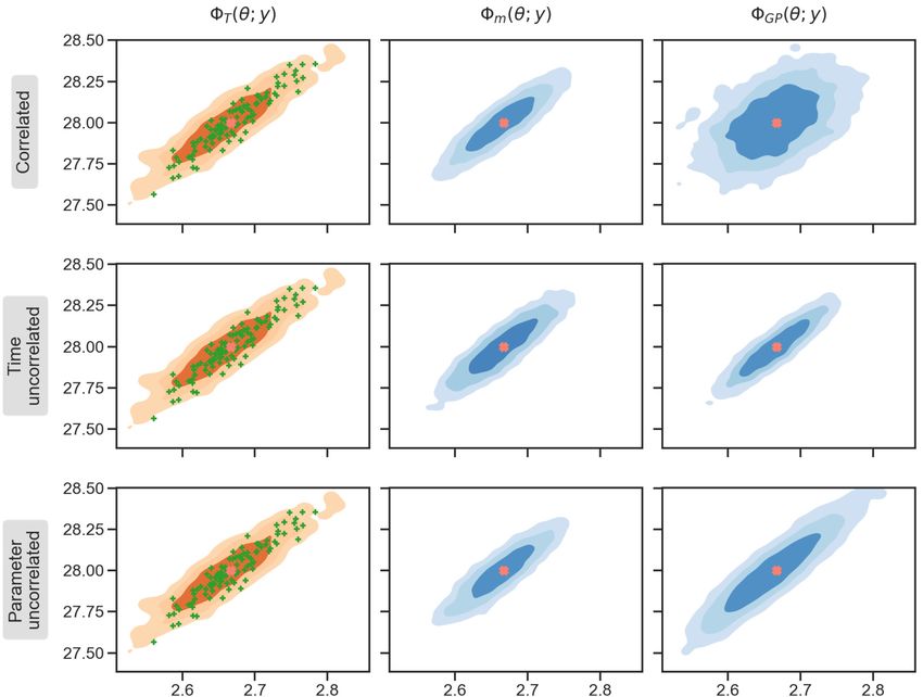
E. Cleary, A. Garbuno-Inigo, S. Lan et al.                                            Journal of Computational Physics 424 (2021) 109716

papers [12,19] and recent contributions are discussed in [2,22,35,70]. But despite their widespread use for both state and
parameter estimation, ensemble Kalman methods do not provide a basis for systematic uncertainty quantification, except in
the Gaussian case [20,48]. This is for two primary reasons: (i) the methods invoke a Gaussian ansatz, which is not always
justified; (ii) they are often employed in situations where evaluation of the underlying dynamical system (state estimation)
or forward model (parameter estimation) is very expensive, and only a small ensemble is feasible. The goal of this paper is
to develop a method that provides a basis for systematic Bayesian uncertainty quantification within inverse problems, build-
ing on the proven power of ensemble Kalman methods. The basic idea is simple: we calibrate the model using variants of
ensemble Kalman inversion; we use the evaluations of the forward model made during the calibration to train an emulator;
we perform approximate Bayesian inversion using Markov Chain Monte Carlo (MCMC) samples based on the (cheap) emu-
lator rather than the original (expensive) forward model. Within this overall strategy, the ensemble Kalman methods may
be viewed as providing a cheap and effective way of determining an experimental design for training an emulator of the
parameter-to-data map to be employed within MCMC-based Bayesian parameter estimation; this is the primary innovation
contained within the paper.

1.1. Literature review

    The ensemble Kalman approach to calibrating unknown parameters to data is reviewed in [35,61], and the imposition of
constraints within the methodology is overviewed in [2]. We refer to this class of methods for calibration, collectively, as
ensemble Kalman inversion (EKI) methods and note that pseudo-code for a variety of the methods may be found in [2]. An
approach to using ensemble-based methods to produce approximate samples from the Bayesian posterior distribution on
the unknown parameters is described in [26]; we refer to this method as ensemble Kalman sampling (EKS). Either of these
approaches, EKI or EKS, may be used in the calibration step of our approximate Bayesian inversion method.
    Gaussian processes (GPs) have been widely used as emulation tools for computationally expensive computer codes [69].
The first use of GPs in the context of uncertainty quantification was proposed in modeling ore reserves in mining [45].
Its motivation was a method to find the best linear unbiased predictor, known as kriging in the geostatistics community
[16,74]. It was later adopted in the field of computer experiments [68] to model possibly correlated residuals. The idea was
then incorporated within a Bayesian modeling perspective [17] and has been gradually refined over the years. Kennedy and
O’Hagan [42] offer a mature perspective on the use of GPs as emulators, adopting a clarifying Bayesian formulation. The use
of GP emulators covers a wide range of applications such as uncertainty analysis [59], sensitivity analysis [60], and computer
code calibration [32]. Perturbation results for the posterior distribution, when the forward model is approximated by a GP,
may be found in [75]. We will exploit GPs for the emulation step of our method which, when informed by the calibration
step, provides a robust approximate forward model. Neural networks [30] could also be used in the emulation step and may
be preferable for some applications of the proposed methodology.
    Bayesian inference is now widespread in many areas of science and engineering, in part because of the development
of generally applicable and easily implementable sampling methods for complex modeling scenarios. MCMC methods [31,
54,55] and sequential Monte Carlo (SMC) [18] provide the primary examples of such methods, and their practical success
underpins the widespread interest in the Bayesian solution of inverse problems [39]. We will employ MCMC for the sampling
step of our method. SMC could equally well be used for the sampling step and will be preferable for many problems;
however, it is a less mature method and typically requires more problem-specific tuning than MCMC.
    The impetus for the development of our approximate Bayesian inversion method is the desire to perform Bayesian inver-
sion on computer models that are very expensive to evaluate, for which derivatives and adjoint calculations are not readily
available and are possibly noisy. Ensemble Kalman inversion methods provide good parameter estimates even with many pa-
rameters, typically with O (102 ) forward model evaluations [40,61], but without systematic uncertainty quantification. While
MCMC and SMC methods provide systematic uncertainty quantification the fact that they require many iterations, and hence
evaluations of the forward model in our setting, is well-documented [29]. Several diagnostics for MCMC convergence are
available [63], and theoretical guarantees of convergence exist [56]. The rate of convergence for MCMC is determined by
the size of the step arising from proposal distribution: short steps are computationally inefficient as the parameter space is
only locally explored whereas large steps lead to frequent rejections and hence to a waste of computational resources (in
our setting forward model evaluations) to generate additional samples. In practice MCMC often requires O (105 ) or more
forward model evaluations [29]. This is not feasible, for example, with climate models [13,37,73].
    In the sampling step of our approximate Bayesian inversion method, we use an emulator that can be evaluated rapidly
in place of the computationally expensive forward model, leading to Bayesian parameter estimation and uncertainty quan-
tification essentially at the computational cost of ensemble Kalman inversion. The ensemble methods provide an effective
design for the emulation, which makes this cheap cost feasible.
    In some applications, the dimension of the unknown parameter is high and it is therefore of interest to understand
how the constituent parts of the proposed methodology behave in this setting. The growing use of ensemble methods
reflects, in part, the empirical fact that they scale well to high-dimensional state and parameter spaces, as demonstrated by
applications in the geophysical sciences [40,61]; thus, the calibrate phase of the methodology scales well with respect to
high input dimension. Gaussian process regression does not, in general, scale well to high-dimensional input variables, but
alternative emulators, such as those based on neural networks [30] are empirically found to do so; thus, the emulate phase
can potentially be developed to scale well with respect to high input dimensions. Standard MCMC methods do not scale well

                                                              2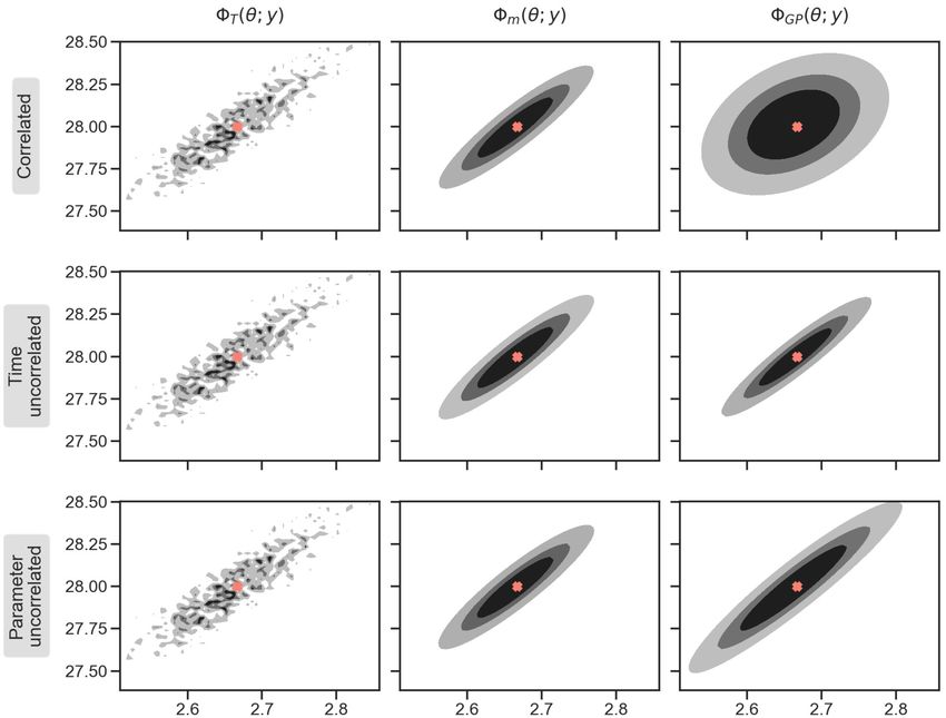
E. Cleary, A. Garbuno-Inigo, S. Lan et al.                                              Journal of Computational Physics 424 (2021) 109716

with respect to high dimensions; see [65] in the context of i.i.d. random variables in high dimensions. However the reviews
[11,15] describe non-traditional MCMC methods which overcome these poor scaling results for high-dimensional Bayesian
inversion with Gaussian priors, or transformations of Gaussians; the paper [41] builds on the ideas in [15] to develop SMC
methods that are efficient in high- and infinite-dimensional spaces. Thus, the sampling phase of the methodology scales
well with respect to high input dimension for appropriately chosen priors.
    There are alternative strategies related to, but different from, the methodology we present in this work. The bulk of these
alternative strategies rely on the adaptive construction of the emulator as the MCMC evolves – learning on the fly [46].
Earlier works have identified the effectiveness of posterior-localized surrogate models, rather than prior-based surrogates in
the setting of Bayesian inverse problems; see [14,50] and the references therein. Within the adaptive surrogate framework,
other type of surrogates have been used such as polynomial chaos expansions (PCE) [76] and deep neural networks [77];
the use of adaptive PCEs has recently been merged with ensemble based algorithms [78]. The effectiveness of all these
works relies on the compromise between exploring the parameter space with the current surrogate and refining it further
where needed; however, as exposed in [14,50,79], the use of an inadequate surrogate leads to biased posterior estimates.
Another strategy for approximate Bayesian inversion can be found in [23] where adaptivity is incorporated within a sparse
quadrature rule used to approximate the integrals needed in the Bayesian inference.

1.2. Our contribution

  • We introduce a practical methodology for approximate Bayesian parameter learning in settings where the parameter-
    to-data map is expensive to evaluate, not easy to differentiate or not differentiable, and where evaluations are possibly
    polluted by noise. The methodology is modular and broken into three steps, each of which can be tackled by different
    methodologies: calibration, emulation, and sampling.
  • In the calibration phase we leverage the power of ensemble Kalman methods, which may be viewed as fast derivative-
    free optimizers or approximate samplers. These methods provide a cheap solution to the experimental design problem
    and ensure that the forward map evaluations are well-adapted to the task of Gaussian process emulation, within the
    context of an outer Bayesian inversion loop via MCMC sampling.
  • We also show that, for problems in which the forward model evaluation is inherently noisy, the Gaussian process
    emulation serves to remove the noise, resulting in a more practical Bayesian inference via MCMC.
  • We demonstrate the methodology with numerical experiments on a model linear problem, on a Darcy flow inverse
    problem, and on the Lorenz ’63 and ’96 models.

   It is worth emphasizing that the idea of emulation within an MCMC loop is not a new one (see citations above) and
that doing so incurs an error which can be controlled in terms of the number of samples used to train the emulator [75].
Similarly the use of EKS to solve inverse problems is not a new idea see [see 2,35, and the references therein]; however,
except in the linear case [72], the error cannot be controlled in terms of the number of ensemble members. What is novel
in our work is the conjunction of the two approaches lifts the EKS from being an, in general uncontrolled but reasonable,
approximator of the posterior into a method which provides controllable approximation of the posterior, in terms of the
number of ensemble members used in the GP training; furthermore the EKS may be viewed intuitively in general, and
provably in the linear case, as providing a good solution to the design problem related to the construction of the emulator.
This is because it tends to concentrate points in the support of the true posterior, even if the points are not distributed
according to the posterior [26].
   In Section 2, we describe the calibrate-emulate-sample methodology introduced in this paper, and in Section 3, we
demonstrate the method on a linear inverse problem whose Bayesian posterior is explicitly known. In Section 4, we study
the inverse problem of determining permeability from pressure in Darcy flow, a nonlinear inverse problem in which the
coefficients of a linear elliptic partial differential equation (PDE) are to be determined from linear functionals of its solution.
Section 5 is devoted to the inverse problem of determining parameters appearing in time-dependent differential equations
from time-averaged functionals of the solution. We view finite time-averaged data as noisy infinite time-averaged data and
use GP emulation to estimate the parameter-to-data map and the noise induced through finite-time averaging. Applica-
tions to the Lorenz’63 and’96 atmospheric science models are described here, and use of the methodology to study an
atmospheric general circulation model is described in the paper [13].

2. Calibrate-emulate-sample

2.1. Overview

    Consider parameters θ related to data y through the forward model G and noise       η:

         y = G (θ) + η.                                                                                                             (2.1)

The inverse problem is to find unknown θ from y, given knowledge of G : R p → Rd and some information about the noise
level such as its size (classical approach) or distribution (statistical approach), but not its value. To formulate the Bayesian

                                                               3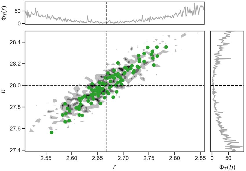
E. Cleary, A. Garbuno-Inigo, S. Lan et al.                                                                    Journal of Computational Physics 424 (2021) 109716

Fig. 1. Schematic of approximate Bayesian inversion method to find θ from y. EKI/EKS produce a small number of approximate (expensive) samples
{θ (m) }m                                                   ( M ) of G , used within MCMC to produce a large number of approximate (cheap) samples {θ (n) } N s ,
          =1 . These are used to train a GP approximation G
        M
                                                                                                                                                           n=1
N s  M.

inverse problem, we assume, for simplicity, that the noise is drawn from a Gaussian with distribution N (0,  y ), that the
prior on θ is a Gaussian N (0, θ ), and that θ and η are a priori independent. If we define1

                       1                     1
          R (θ) =  y − G (θ)2 y + θ2θ ,                                                                                                            (2.2)
                       2                     2
the posterior on θ given y has density


         π y (θ) ∝ exp − R (θ) .                                                                                                                         (2.3)

     In a class of applications of particular interest to us, the data y comprises statistical averages of observables. The map
G (θ) provides the corresponding statistics delivered by a model that depends on θ . In this setting the assumption that the
noise be Gaussian is reasonable if y and G (θ) represent statistical aggregates of quantities that vary in space and/or time.
Additionally, we take the view that parameters θ  for which Gaussian priors are not appropriate (for example because they
are constrained to be positive) can be transformed to parameters θ for which Gaussian priors make sense.
    We use EKS with J ensemble members and N iterations (time-steps of a discretized continuous time algorithm) to
generate approximate samples from (2.3), in the calibration step of the methodology. This gives us J N parameter–model
                                     JN
evaluation pairs {θ (m) , G (θ (m) )}m=1 which we can use to produce an approximation of G in the GP emulation step of the
algorithm. Whilst the methodology of optimal experimental design can be used, in principle, as the basis for choosing
parameter-data pairs for the purpose of emulation [3] it can be prohibitively expensive. The theory and numerical results
shown in [26] demonstrate that EKS distributes particles in regions of high posterior probability; this is because it approx-
imates a mean-field interacting particle system with invariant measure equal to the posterior probability distribution (2.3).
Using the EKS thus provides a cheap and effective solution to the design problem, producing parameter–model evaluation
pairs that are well-positioned for the task of approximate Bayesian inversion based on the (cheap) emulator. In practice it
is not always necessary to use all J N parameter–model evaluation pairs but to instead use a subset of size M ≤ J N; we
denote the resulting GP approximation of G by G ( M ) . Throughout this paper we simply take M = J and use the output of
the EKS in the last step of the iteration as the design. However other strategies, such as decreasing J and using all or most
of the N steps, are also feasible.
    G (M ) in place of the (expensive) forward model G . With the emulator G (M ) , we define the modified inverse problem of
finding parameter θ from data y when they are assumed to be related, through noise η , by

         y = G ( M ) (θ) + η.

This is an approximation of the inverse problem defined by (2.1). The approximate posterior on θ given y has density
π (M ) defined by the approximate log likelihood arising from this approximate inverse problem. In the sample step of the
methodology, we apply MCMC methods to sample from π ( M ) .
    The overall framework, comprising the three steps calibrate, emulate, and sample is cheap to implement because it
involves a small number of evaluations of G (·) (computed only during the calibration phase, using ensemble methods
where no derivatives of G (·) are required), and because the MCMC method, which may require many steps, only requires
evaluation of the emulator G ( M ) (·) (which is cheap to evaluate) and not G (·) (which is assumed to be costly to evaluate
and is possibly only known noisily). On the other hand, the method has ingredients that make it amenable to produce a
controlled approximation of the true posterior. This is true since the EKS steps generate points concentrating near the main
support of the posterior so that the GP emulator provides an accurate approximation of G (·) where it matters.2 A depiction
of the framework and the algorithms involved can be found in Fig. 1. In the rest of the paper, we use the acronym CES to
denote the three step methodology. Furthermore we employ boldface on one letter when we wish to emphasize one of the
three steps: calibration is emphasized by (CES); emulation by (CES); and sampling by (CES).

                                                                                           1      1                     1
 1
     For any positive-definite symmetric matrix A, we define a, a A = a, A −1 a = A − 2 a, A − 2 a and a A =  A − 2 a.
 2
     By “main support” we mean a region containing the majority of the probability.

                                                                               4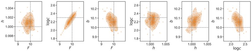
E. Cleary, A. Garbuno-Inigo, S. Lan et al.                                                                                  Journal of Computational Physics 424 (2021) 109716

2.2. Calibrate – EKI and EKS

   The use and benefits of ensemble Kalman methods to solve inverse or parameter calibration problems have been outlined
in the introduction. We will employ particular forms of the ensemble Kalman inversion methodology that we have found
to perform well in practice and that are amenable to analysis; however, other ensemble methods to solve inverse problems
could be used in the calibration phase.
   The basic EKI method is found by time-discretizing the following system of interacting particles [71]:

                            1
                             J
         dθ ( j )
                     =−                G (θ (k) ) − Ḡ , G (θ ( j ) ) − y       y     (θ (k) − θ̄),                                                                       (2.4)
           dt               J
                                k =1

where θ̄ and Ḡ denote the sample means given by

                   1  (k)                         1
                     J                              J
         θ̄ =          θ ,                  Ḡ =                  G (θ (k) ).                                                                                              (2.5)
                   J                                   J
                     k =1                                  k =1

                                                                       J
For use below, we also define  = {θ ( j ) } j =1 and the p × p matrix

                       1
                        J
         C() =                    (θ (k) − θ̄ ) ⊗ (θ (k) − θ̄ ).                                                                                                          (2.6)
                       J
                            k =1

The dynamical system (2.4) drives the particles to consensus, while also driving them to fit the data and hence solve the
inverse problem (2.1). Time-discretizing the dynamical system leads to a form of derivative-free optimization to minimize
the least squares misfit defined by (2.1) [35,71].
   An appropriate modification of EKI, to attack the problem of sampling from the posterior π y given by (2.3), is EKS [26].
Formally this is obtained by adding a prior-related damping term, as in [10], and a -dependent noise to obtain

                            1
                             J
         dθ ( j )                                                                                                                     dW ( j )
                     =−                G (θ (k) ) − Ḡ , G (θ ( j ) ) − y       y     (θ (k) − θ̄) − C()− 1 ( j)
                                                                                                           θ θ      +     2C()                  ,                         (2.7)
           dt               J                                                                                                           dt
                                k =1

where the { W ( j ) } are a collection of i.i.d. standard Brownian motions in the parameter space R p . The resulting interacting
particle system approximates a mean-field Langevin-McKean diffusion process which, for linear G , is invariant with respect
to the posterior distribution (2.3) and, more generally, concentrates close to it; see [26] and [25] for details. The specific
algorithm that we implement here time-discretizes (2.7) by means of a linearly implicit split-step scheme given by [26]

                                           1
                                            J
                                                                                                         − tn C(n ) −
           (∗, j )      ( j)                                   (k)              ( j)               (k)                   1  (∗, j )
         θn+1 = θn − tn                                   G (θn ) − Ḡ , G (θn ) − y          y θn                   θ θn+1 ,                                        (2.8a)
                                            J
                                                k =1
            ( j)        (∗, j )
                                                                    ( j)
          θn+1 = θn+1 +                    2 tn C(n ) ξn ,                                                                                                           (2.8b)
           ( j)
where ξn ∼ N(0, I ), θ is the prior covariance and tn is an adaptive timestep given in [26], and based on methods devel-
oped for EKI in [44]. This is a split-step method for the SDE (2.7) which is linearly implicit and ensures approximation of the
Itô interpretation of the equation; other discretizations can be used, provided they are consistent with the Itô interpretation.
The finite J correction to (2.7) proposed in [58], and further developed in [25], can easily be incorporated into the explicit
step of this algorithm, and other time-stepping methods can also be used.

2.3. Emulate – GP emulation

                                                                                                                                                       (i )     (i )   J
   The ensemble-based algorithm described in the preceding subsection produces input-output pairs {θn , G (θn )}i =1 for
n = 0, . . . , N. For n = N and J large enough, the samples of θ are approximately drawn from the posterior distribution. We
use a subset of cardinality M ≤ J N of this design as training points to update a GP prior to obtain the function G ( M ) (·) that
will be used instead of the true forward model G (·). The cardinality M denotes the total number of evaluations of G used
in training the emulator G ( M ) . Recall that throughout this paper we take M = J and use the output of the EKS in the last
step of the iteration as the design.
   The forward model is a multioutput map G : R p → Rd . It often suffices to emulate each output coordinate l = 1, . . . , d
independently; however, variants on this are possible, and often needed, as discussed at the end of this subsection. For the
moment, let us consider the emulation of the l-th component in G (θ); denoted by Gl (θ). Rather than interpolate the data,

                                                                                                  5
E. Cleary, A. Garbuno-Inigo, S. Lan et al.                                                            Journal of Computational Physics 424 (2021) 109716

we assume that the input-output pairs are polluted by additive noise.3 We place a Gaussian process prior with zero or
linear mean function on the l-th output of the forward model and, for example, use the squared exponential kernel

                             1
         kl (θ, θ ) = σ exp − θ − θ  D l + λl2 δθ (θ  ),

                           l
                            2        2
                                                                                                                                                 (2.9)
                                             2
                                                                           √              (l)   (l)
where σl denotes the amplitude of the covariance kernel;           D l = diag( 1 , . . . , p ) is the diagonal matrix of lengthscale
parameters; δx ( y ) is the Kronecker delta function; and λl the standard deviation of the observation process. The hyperpa-
rameters φl = (σl2 , D l , λl2 ), which are learnt from the input-output pairs along with the regression coefficients of the GP,
account for signal strength (σl2 ); sensitivity to changes in each parameter component ( D l ); and the possibility of white
noise with variance λl2 in the evaluation of the l-th component of the forward model Gl (·). We adopt an empirical Bayes
approach to learn the hyperparameters of each of the d Gaussian processes.
   The final emulator is formed by stacking each of the GP models in a vector,

         G ( M ) (θ) ∼ N (m(θ), GP (θ)) .                                                                                                      (2.10)

The noise η typically found in (2.1) needs to be incorporated along with the noise                    ηGP (θ) ∼ N (0, GP (θ)) in the emulator
G (M ) (θ), resulting in the inverse problem

         y = m(θ) + ηGP (θ) + η.                                                                                                                (2.11)

   We assume that ηGP (θ) and η are independent of one another. In some cases, one or other of the sources of noise
appearing in (2.11) may dominate the other and we will then neglect the smaller one. If we neglect η , we obtain the
negative log-likelihood

                          1                        1
         (GPM ) (θ) =  y − m(θ)2GP (θ ) +          log det GP (θ);                                                                         (2.12)
                          2                        2
for example, in situations where initial conditions of a dynamical systems are not known exactly. This situation is encoun-
tered in applications where G is defined through time-averaging, as in Section 5; in these applications the noise ηGP (θ)
is the major source of uncertainty and we take η = 0. If, on the other hand, we neglect ηGP then we obtain negative
log-likelihood

                          1
         (mM ) (θ) =  y − m(θ)2 y .                                                                                                         (2.13)
                          2
If both noises are incorporated, then (2.12) is modified to give

                          1                             1
         (GPM ) (θ) =  y − m(θ)2GP (θ )+ y +           log det GP (θ) +  y ;                                                             (2.14)
                          2                             2
this is used in Section 4.
   We note that the specifics of the GP emulation could be adapted – we could use correlations in the output space Rd ,
other kernels, other mean functions, and so forth. A review of multioutput emulation in the context of machine learning can
be found in [4] and references therein; specifics on decorrelating multioutput coordinates can be found in [33]; and recent
advances in exploiting covariance structures for multioutput emulation in [8,9]. For the sake of simplicity, we will focus on
emulation techniques that preserve the strategy of determining, and then learning, approximately uncorrelated components;
methodologies for transforming variables to achieve this are discussed in Appendix A.

2.4. Sample – MCMC

   For the purposes of the MCMC algorithm, we need to initialize the Markov chain and choose a proposal distribution.
The Markov chain is initialized with θ0 drawn from the support of the posterior; this ensures that the MCMC has a short
transient phase. To initialize, we use the ensemble mean of the EKS at the last iteration, θ̄ J . For the MCMC step we use
a proposal of random walk Metropolis type, employing a multivariate Gaussian distribution with covariance given by the
empirical covariance of the ensemble from EKS. We are thus pre-conditioning the sampling phase of the algorithm with
approximate information about the posterior from the EKS. The resulting MCMC method is summarized in the following
                                                                     N
steps and is iterated until a desired number N s  J of samples {θn }n=s 1 is generated:

  1. Choose θ0 = θ̄ J .
  2. Propose a new parameter choice θn∗+1 = θn + ξn where ξn ∼ N (0, C ( J )).

 3
     The paper [5] interprets the use of additive noise within computer code emulation.

                                                                            6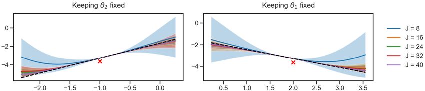
E. Cleary, A. Garbuno-Inigo, S. Lan et al.                                                                           Journal of Computational Physics 424 (2021) 109716

Fig. 2. Density estimates for different ensemble sizes used for the calibration step. Leftmost panel show the true posterior distribution. The green dots show
the EKS at the 20-th iteration. The contour levels show the density of a Gaussian with mean and covariance estimated from EKS at said iteration. (For
interpretation of the colors in the figure(s), the reader is referred to the web version of this article.)

  3. Set θn+1 = θn∗+1 with probability a(θn , θn∗+1 ); otherwise set θn+1 = θn .
  4. n → n + 1, return to 2.

The acceptance probability is computed as:

                   ∗                                             1                                     1
         a(θ, θ ) = min 1, exp                   ·( M ) (θ ∗ ) + θ ∗ 2θ       −       ·( M ) (θ) + θ2θ       ,                                         (2.15)
                                                                2                                     2
            (M )
where ·           is defined in (2.12), (2.13) or (2.14), whichever is appropriate.

3. Linear problem

   By choosing a linear parameter-to-data map, we illustrate the methodology in a case where the posterior is Gaussian
and known explicitly. This demonstrates both the viability and accuracy of the method in a transparent fashion.

3.1. Linear inverse problem

   We consider a linear forward map G (θ) = G θ , with G ∈ Rd× p . Each row of the matrix G is a p-dimensional draw from
a multivariate Gaussian distribution. Concretely we take p = 2 and each row G i ∼ N(0, ), where 12 = 21 = −0.9, and
11 = 22 = 1. The synthetic data we have available to perform the Bayesian inversion is then given by

         y = G θ † + η,                                                                                                                                          (3.1)

where θ † = [−1, 2] , and η ∼ N(0, ) with  = 0.12 I .
   We assume that, a priori, parameter θ ∼ N(mθ , θ ). In this linear Gaussian setting the solution of the Bayesian linear
inverse problem is itself Gaussian [see 27, Part IV] and given by the Gaussian distribution

                                    1
         π y (θ) ∝ exp − θ − mθ | y 2θ | y ,                                                                                                                 (3.2)
                                    2
where mθ| y and θ| y denote the posterior mean and covariance. These are computed as

         −  1      −1      −1
          θ | y = G  y G + θ ,                     mθ | y = θ | y G  − 1    −1
                                                                          y y + θ mθ .                                                                         (3.3)

3.2. Numerical results

   For the calibration step (CES) we consider the EKS algorithm. Fig. 2 shows how the EKS samples estimate the posterior
distribution (the far left). The green dots correspond to 20-th iteration of EKS with different ensemble sizes. We also display
in gray contour levels the density corresponding to the 67%, 90% and 99% probability levels under a Gaussian with mean
and covariance estimated from EKS at said 20-th iteration. This allows us to visualize the difference between the results
of EKS and the true posterior distribution in the leftmost panel. In this linear case, the mean-field limit of EKS exactly
reproduces the invariant measure [26]. The mismatch between the EKS samples and the true posterior can be understood
from the fact that time discretizations of Langevin diffusions are known to induce errors if no metropolization scheme is
added to the dynamics [49,64,66], and from the finite number of particles used; the latter could be corrected by using the
ideas introduced in [58] and further developed in [25].
   The GP emulation step (CES) is depicted in Fig. 3 for one component of G . Each GP is trained using the 20-th iteration of
EKS for each ensemble size. We employ a zero mean GP with the squared-exponential kernel (2.9). We add a regularization
term to the lengthscales of the GP by means of a prior in the form of a Gamma distribution. This is common in GP
Bayesian inference when the domain of the input variables is unbounded. The choice of this regularization ensures that the

                                                                                          7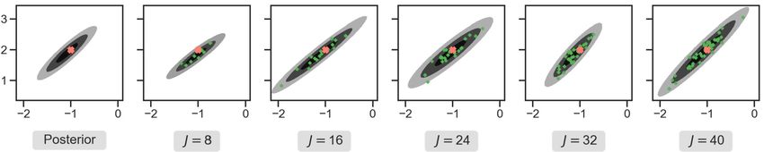
E. Cleary, A. Garbuno-Inigo, S. Lan et al.                                                                Journal of Computational Physics 424 (2021) 109716

Fig. 3. Gaussian process emulators learnt using different training datasets. The input-output pairs are obtained from the calibration step using EKS. Each
color for the lines and the shaded regions correspond to different ensemble sizes as described in the legend.

Fig. 4. Density of a Gaussian with mean and covariance estimated from GP-based MCMC samples using M = J design points. The true posterior distribution
is shown in the far left. Each GP-based MCMC generated 2 × 10⁴ samples. These samples are not shown for clarity.

                            Table 1
                            Averaged mean square error of the posterior location (mean) computed from 20 independent realizations.

                              Ensemble size           8                16               24               32               40
                              EKS                     0.1171           0.0665           0.0528           0.0584           0.0648
                              CES                     0.0652           0.0219           0.0125           0.0122           0.0173

                            Table 2
                            Averaged mean square error of the posterior spread (covariance) computed by means of the Frobenius
                            norm and 20 independent realizations.

                              Ensemble size           8                16               24               32               40
                              EKS                     0.1010           0.0703           0.0937           0.0868           0.0664
                              CES                     0.0555           0.0241           0.0092           0.0050           0.0056

covariance kernels, which are regression functions for the mean of the emulator, decay fast away from the data, and that no
short variations below the levels of available data are introduced [27,28]. We can visualize the emulator of the component
of the linear system considered here by fixing one parameter at the true value while varying the other. The dashed reference
in Fig. 3 shows the model G θ . The red cross denotes the corresponding observation. The solid lines correspond to the mean
of the GP, while the shaded regions contain 2 standard deviations of predicted variability. Colors correspond to different
ensemble sizes as described in the figure’s legend. We can see in Fig. 3 that the GP increases its accuracy as the amount
of training data is increased. In the end, for training sets of size J ≥ 16, it correctly simulates the linear model with low
uncertainty in the main support of the posterior.
    Fig. 4 depicts results in the sampling step (CES). These are obtained by using a GP approximation of G θ within MCMC.
The GP-based MCMC uses (2.14) since the forward model is deterministic and the data is polluted by noise. The contour
levels show a Gaussian distribution with mean and covariance estimated from N s = 2 × 10⁴ GP-based MCMC samples (not
shown) in each of the different ensemble settings. The results show that the true posterior is captured with an ensemble
size of 16 or more. Moreover, Table 1 shows the mean square error of the posterior location parameter in (3.3); that
is, the error in Euclidean norm of the sample-based mean. This error is computed by means of the ensemble mean and
the analytic posterior mean (top row), and the CES posterior mean and the analytic solution (bottom row). Analogously,
Table 2 shows the mean square error for the spread; that is, the Frobenius norm error in the sample-based covariance
matrix – both computed from the EKS and CES samples, top and bottom rows, respectively – and the analytic solution for
the posterior covariance in (3.3). For both parameters, it can be seen that the CES-approximated posterior achieves higher
accuracy relative to the EKS alone. For this linear problem both methods provably recover the true posterior distribution, in
the limit of large ensemble size, so that it is interesting to see that the CES-approximated posterior improves upon the EKS
alone. Recall from the discussion in Subsection 1.2, however, that for nonlinear problems EKS does not in general recover the
posterior distribution, whilst the CES-approximated posterior converges to the true posterior distribution as the number of
training samples increases, regardless of the distribution of the EKS particles; what is beneficial, in general, about using EKS

                                                                                8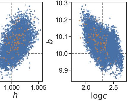
E. Cleary, A. Garbuno-Inigo, S. Lan et al.                                                                  Journal of Computational Physics 424 (2021) 109716

to design the GP is that the samples are located close to the support of the true posterior, even if they are not distributed
according to the posterior.

4. Darcy flow

   In this section, we apply our methodology to a PDE nonlinear inverse problem arising in porous medium flow: the
determination of permeability from measurements of the pressure (piezometric head).

4.1. Elliptic inverse problem

4.1.1. Forward problem
    The forward problem is to find the pressure field p in a porous medium defined by the (for simplicity) scalar permeability
field a. Given a scalar field f defining sources and sinks of fluid, and assuming Dirichlet boundary conditions for p on the
domain D = (0, 1)2 , we obtain the following elliptic PDE determining the pressure from permeability:

         −∇ · (a(x)∇ p (x)) = f (x),                          x ∈ D.                                                                                  (4.1a)
                                   p (x) = 0,               x ∈ ∂ D.                                                                                  (4.1b)

   In this paper we always take f ≡ 1. The unique solution of the equation implicitly defines a map from a ∈ L ∞ ( D ; R) to
p ∈ H 01 ( D ; R).

4.1.2. Inverse problem
    We assume that the permeability is dependent on unknown parameters θ ∈ R p , so that a(x) = a(x; θ) > 0 almost
everywhere in D. The inverse problem of interest is to determine θ from noisy observations of d linear functionals (mea-
surements) of p (x; θ). Thus,

         G j (θ) =     j       p (·; θ) + η,                   j = 1, · · · , d .                                                                      (4.2)
                                                                                                                2
We assume the additive noise η to be a mean zero Gaussian with covariance equal to γ I . Throughout this paper, we work
with pointwise measurements so that j ( p ) = p (x j ).4 We employ d = 50 measurement locations chosen at random from a
uniform grid in the interior of D.
   We introduce a log-normal parameterization of a(x; θ) as follows:

         log a(x; θ) =                   θ          λ ϕ (x)                                                                                            (4.3)
                                   ∈Kq

where

         ϕ (x) = cos π , x ,                               λ = (π 2 | |2 + τ 2 )−α ;                                                                   (4.4)

the smoothness parameters are assumed to be τ = 3, α = 2, and K q ⊂ K ≡ Z2 is the set, with finite cardinality | K q | = q,
of indices over which the random series is summed. A priori we assume that θ ∼ N(0, 1) so that we have a Karhunen-
Loève representation of a as a log–Gaussian random field [62]. We often find it helpful to write (4.3) as a sum over a
one-dimensional variable rather than a lattice:

         log a(x; θ  ) =                   θk       λk ϕk (x).                                                                                     (4.5)
                                   k∈ Z q

Throughout this paper we choose K q , and hence Z q , to contain the q largest {λ }. We order the indices in Z q ⊂ Z+ so that
the set of {λk } are non-increasing with respect to k.

4.2. Numerical results

   We generate an underlying true random field by sampling θ † ∈ R p from a standard multivariate Gaussian distribu-
tion, N(0, I p ), of dimension p = 162 = 256. This is used as the coefficients in (4.3) by means of the re-labeling (4.5). The
evaluation of the forward model G (θ) requires solving the PDE (4.1b) for a given realization of the random field a. This
is done with a cell-centered finite difference scheme [6,67]. We create data y from (4.2) with a random perturbation

 4
    The implied linear functionals are not elements of the dual space of H 01 ( D ; R) in dimension 2 but mollifications of them are. In practice, mollification
with a narrow kernel does not affect results of the type presented here [36], and so we do not use it.

                                                                                       9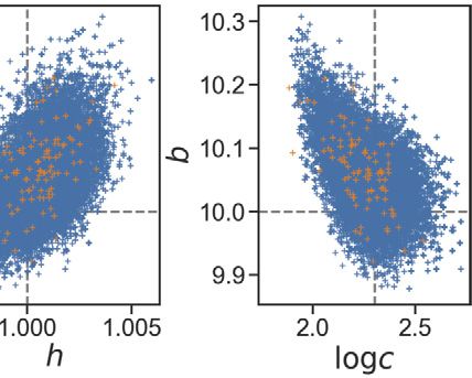
E. Cleary, A. Garbuno-Inigo, S. Lan et al. Journal of Computational Physics 424 (2021) 109716
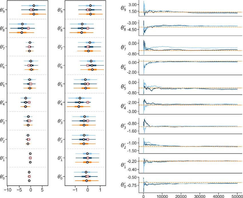
Fig. 5. Results of CES in the Darcy flow problem. Colors throughout the panel denote results using different calibration and GP training settings. This are:
light blue – ensemble of size J = 128; dark blue – ensemble of size J = 512; and orange, the MCMC gold standard. Left panel shows each θ component
for CES. The middle panel shows the same information, but using standardized components of θ . The interquartile range is displayed with a thick line; the
95% credible intervals with a thin line; and the median with circles. The right panel shows typical MCMC running averages, demonstrating stationarity of
the Markov chain.
η ∼ N(0, 0.0052 × I d ), where I d denotes the identity matrix. The locations for the data, and hence the evaluation of the
forward model, were chosen at random from the 162 computational grid used to solve the Darcy flow. For the Bayesian
inversion we use a truncation of (4.5) with p < p terms, allowing us to avoid the inverse crime of using the same model
that generated the data to solve the inverse problem [39]. Specifically, we consider p = 10. We employ a non-informative
centered Gaussian prior with covariance θ = 102 × I p ; this is also used to initialize the ensemble for EKS. We consider
ensembles of size J ∈ {128, 512}.
We perform the complete CES procedure starting with EKS as described above for the calibration step (CES). The em-
ulation step (CES) uses a GP with a linear mean Gaussian process with squared-exponential kernel (2.9). Empirically, the
linear mean allows us to capture a significant fraction of the relevant parameter response. The GP covariance matrix GP (θ)
accounts for the variability of the residuals from the linear function. The sampling step (CES) is performed using the Ran-
dom Walk procedure described in Section 2.4; a Gaussian transition distribution is used, found by matching to the first two
moments of the ensemble at the last iteration of EKS. In this experiment, the likelihood (2.14) is used because the forward
model is a deterministic map, and we have data polluted by additive noise.
We compare the results of the CES procedure with those obtained from a gold standard MCMC employing the true
forward model. The results are summarized in Fig. 5. The right panel shows typical MCMC running averages, suggesting
stationarity of the Markov chain. The left panel shows the forest plot of each θ component. The middle panel shows
the standardized components of θ . These forest plots show the interquartile range with a thick line; the 95% credible
intervals with a thin line; and the median with circles. The true value of the parameters are denoted by red crosses. The
results demonstrate that the CES methodology accurately reproduces the true posterior using calibration and training with
M = J = 512 ensemble members. For the smaller ensemble, M = J = 128 there is a visible systematic deviation in some
components, like θ7 . However, the CES posterior does capture the true value. Note that the gold standard MCMC employs
10E. Cleary, A. Garbuno-Inigo, S. Lan et al. Journal of Computational Physics 424 (2021) 109716
Fig. 6. Forward UQ exercise of exceedance on both the pressure field, p (·) > p̄, and permeability field, a(·) > ā. Both threshold levels are obtained from the
forward model at the truth θ † and taking the median across the locations (4.2). The PDFs are constructed by running the forward model on a small set of
samples, N UQ = 250, and computing the number of lattice points exceeding the threshold. The samples are obtained by using the CES methodology (light
blue – CES with M = J = 128, and dark blue – CES with M = J = 512). The samples in orange are obtained from a gold standard MCMC using the true
forward model within the likelihood, rather than the emulator.
uses tens of thousands of evaluations of the map from θ to y, where as the CES methodology requires only hundreds, and
yet produces similar results.
The results from the CES procedure are also used in a forward UQ setting: posterior variability in the permeability is
pushed forward onto quantities of interest. For this purpose, we consider exceedances on the pressure and permeability
fields above certain thresholds. These thresholds are computed from the observed data by taking the median across the
50 available locations (4.2). The forward model (4.1b) is solved with N UQ = 500 different parameter settings coming from
samples of the CES Bayesian posterior. We also show the comparison with the gold standard using the true forward model.
We evaluate the pressure and the permeability field at each lattice point, denoted by ∈ K q , and compare with the observed
threshold levels computed from the 50 available locations, denoted by j in (4.2). We record the number of lattice points
exceeding such bounds for each of the N UQ samples. Fig. 6 shows the corresponding KDE for the probability density function
(PDF) in this forward UQ exercise. The orange lines correspond to the PDF of the number of points in the lattice that
exceed the threshold computed from the samples drawn using MCMC with the Darcy flow model. The corresponding PDFs
associated to the CES posterior, based on calibration and emulation using different ensemble sizes, are shown in different
blue tonalities (light blue – CES with M = J = 128, and dark blue – CES with M = J = 512). We use a k-sample Anderson–
Darling test to find evidence against the null hypothesis that assumes that the forward UQ samples using the CES procedure
are statistically similar to samples from the true distribution. This test is non-parametric and relies on the comparison of
the empirical cumulative functions [43, See Ch. 13]. Applying the k-sample Anderson–Darling test at 5% significance level for
the M = J = 128 case, shows evidence to reject the null hypothesis of the samples being drawn from the same distribution
in the pressure exceedance forward UQ. This means that with such limited number of forward model evaluations, the CES
procedure is not able to generate samples that seem to be generated from the true distribution. In the case of having more
forward model evaluations, such test does not provide statistical evidence to reject the hypothesis that the distributions are
similar to the one based on the Darcy model.
5. Time-averaged data
In parameter estimation problems for chaotic dynamical systems, such as those arising in climate modeling [13,37,73],
data may only be available in time-averaged form; or it may be desirable to study time-averaged quantities in order to
ameliorate difficulties arising from the complex objective functions, with multiple local minima, which arise from trying
to match trajectories [1]. Indeed the idea fits the more general framework of feature-based data assimilation introduced in
[57] which, in turn, is closely related to the idea of extracting sufficient statistics from the raw data [24]. The methodology
developed in this section underpins similar work conducted for a complex climate model described in the paper [13].
5.1. Inverse problems from time-averaged data
The problem is to estimate the parameters θ ∈ R p of a dynamical system evolving in Rm from data y comprising
time-averages of an Rd −valued function ϕ (·). We write the dynamical system as
ż = F ( z; θ), z(0) = z0 . (5.1)
Since z(t ) ∈ R and θ ∈ R we have F : R × R → R and ϕ : R → R . We will write z(t ; θ) when we need to
m p m p m m d
emphasize the dependence of a trajectory on θ . In view of the time-averaged nature of the data it is useful to define the
operator
11E. Cleary, A. Garbuno-Inigo, S. Lan et al. Journal of Computational Physics 424 (2021) 109716
T0 +τ
1
Gτ (θ; z0 ) = ϕ (z(t ; θ))dt (5.2)
τ
T0
where T 0 is a predetermined spinup time, τ is the time horizon over which the time-averaging is performed, and z0 the
initial condition of the trajectory used to compute the time-average. Our approach proceeds under the following assump-
tions:
Assumptions 1. The dynamical system (5.1) satisfies:
1. For every θ ∈ , (5.1) has a compact attractor A, supporting an invariant measure μ(dz; θ). The system is ergodic,
and the following limit – a Law of Large Numbers (LLN) analogue – is satisfied: for z0 chosen at random according to
measure μ(·; θ) we have, with probability one,
lim Gτ (θ; z0 ) = G (θ) := ϕ (z)μ(dz; θ). (5.3)
τ →∞
A
2. We have a Central Limit Theorem (CLT) quantifying the ergodicity: for z0 distributed according to μ(dz; θ),
1
Gτ (θ; z0 ) ≈ G (θ) + √ N(0, (θ)). (5.4)
τ
In particular, the initial condition plays no role in time averages over the infinite time horizon. However, when finite
time averages are employed, different random initial conditions from the attractor give different random errors from the
infinite time-average, and these, for fixed spinup time T 0 , are approximately Gaussian. Furthermore, the covariance of the
Gaussian depends on the parameter θ at which the experiment is conducted. This is reflected in the noise term in (5.4).
Here we will assume that the model is perfect in the sense that the data we are presented with could, in principle,
be generated by (5.1) for some value(s) of θ and z0 . The only sources of uncertainty come from the fact that the true
value of θ is unknown, as is the initial condition z0 . In many applications, the values of τ that are feasible are limited by
computational cost. The explicit dependence of Gτ on τ serves to highlight the effect of τ on the computational budget
required for each forward model evaluation. Use of finite time-averages also introduces the unwanted nuisance variable z0
whose value is typically unknown, but not of intrinsic interest. Thus, the inverse problem that we wish to solve is to find θ
solving the equation
y = G T (θ; z0 ) (5.5)
where z0 is a latent variable and T is the computationally-feasible time window we can integrate the system (5.1). We
observe that the preceding considerations indicate that it is reasonable to assume that
y = G (θ) + η, (5.6)
where η ∼ N(0, y (θ)) and y (θ) = T −1 (θ). We will estimate
y (θ) in two ways: firstly using long-time series data; and
secondly using a GP informed by forward model evaluations.
We first estimate y (θ) directly from Gτ with τ T . We will not employ θ− dependence in this setting and simply
estimate a fixed covariance obs . This is because, in the applications we envisage such as climate modeling [13], long time-
series data over time-horizon τ will typically be available only from observational data. The cost of repeatedly simulating
at different candidate θ values is computationally prohibitive, in contrast, to simulations over a shorter time-horizon T .
( j)
We apply EKS to make an initial calibration of θ from y given by (5.5), using G T (θ ( j ) ; z0 ) in place of G (θ ( j ) ) and obs in
( j)
place of y (·), within the discretization (2.8) of (2.7). We find the method to be insensitive to the exact choice of z0 , and
typically use the final value of the dynamical system computed in the preceding step of the ensemble Kalman iteration.
We then take the evaluations of G T as noisy evaluations of G , from which we learn the Gaussian process G ( M ) . We use the
mean m(θ) of this Gaussian process as an estimate of G . Our second estimate of y (θ) is obtained by using the covariance
of the Gaussian process GP (θ). We can evaluate the misfit through either of the expressions
1
m (θ; y ) = y − m(θ)2obs , (5.7a)
2
1 1
GP (θ; y ) = y − m(θ)2GP (θ ) + log det GP (θ). (5.7b)
2 2
Note that equations (5.7) are the counterparts of (2.12) and (2.13) in the setting with time-averaged data. In what follows,
we will contrast these misfits, both based on the learnt GP emulator, with the misfit that uses the noisy evaluations G T
directly. That is, we use the misfit computed as
12E. Cleary, A. Garbuno-Inigo, S. Lan et al. Journal of Computational Physics 424 (2021) 109716
Fig. 7. Contour levels of the misfit of the Lorenz’63 forward model corresponding to (67%, 90%, 99%) density levels. The dotted lines shows the locations of
the true parameter values that generated the data. The green dots shows the final ensemble of the EKS algorithm. The marginal plots show the misfit as
a 1-d function keeping one parameter fixed at the truth while varying the other. This highlights the noisy response from the time-average forward model
GT .
1
T (θ; y ) = y − GT (θ)2obs . (5.8)
2
In the latter, dependence of G T on initial conditions is suppressed.
5.2. Numerical results – Lorenz’63
We consider the 3-dimensional Lorenz equations [52]
ẋ1 = σ (x2 − x1 ), (5.9a)
ẋ2 = rx1 − x2 − x1 x3 , (5.9b)
ẋ3 = x1 x2 − bx3 , (5.9c)
with parameters σ , b, r ∈ R+ . Our data is found by simulating (5.9) with (σ , b, r ) = (10, 28, 8/3), a value at which the
system exhibits chaotic behavior. We focus on the inverse problem of recovering (r , b), with σ fixed at its true value of 10,
from time-averaged data.
Our statistical observations are first and second moments over time windows of size T = 10. Our vector of observations
is computed by taking ϕ : R3 → R9 to be
ϕ (x) = (x1 , x2 , x3 , x21 , x22 , x23 , x1 x2 , x2 x3 , x3 x1 ). (5.10)
This defines G T . To compute obs we used time-averages of ϕ (x) over τ = 360 units of time, at the true value of θ ; we split
the time-series into windows of size T and neglect an initial spinup of T 0 = 30 units of time. Together G T and obs produce
a noisy function T as depicted in Fig. 7. The noisy nature of the energy landscape, demonstrated in this figure, suggests
that standard optimization and MCMC methods may have difficulties; the use of GP emulation will act to smooth out the
noise and lead to tractable optimization and MCMC tasks.
For the calibration step (CES), we run the EKS using the estimate of = obs within the algorithm (2.7), and within
the misfit function (5.8), as described in Section 5.1. We assumed the parameters to be a priori governed by an isotropic
Gaussian prior in logarithmic scale. The mean of the prior is m0 = (3.3, 1.2) and its covariance is 0 = diag(0.152 , 0.52 ).
This gives broad priors for the parameters with 99% probability mass in the region [20, 40] × [0, 15]. The results of evolving
the EKS through 11 iterations can be seen in Fig. 7, where the green dots represent the final ensemble. The dotted lines
locate the true underlying parameters in the (r , b) space.
13E. Cleary, A. Garbuno-Inigo, S. Lan et al. Journal of Computational Physics 424 (2021) 109716
Fig. 8. Contour levels of the Lorenz’63 posterior distribution corresponding to (67%, 90%, 99%) density levels. For each row we depict: in the left panel, the
contours using the true forward model; in the middle panel, the contours of the misfit computed as m (5.7a); and in the right panel, the contours of
the misfit obtained using GP (5.7b). The difference between rows is due to the decorrelation strategy used to learn the GP emulator, as indicated in the
leftmost labels. The GP-based densities show an improved estimation of uncertainty arising from GP estimation of the infinite time-averages, in comparison
with employing the noisy exact finite time averages, for both decorrelation strategies.
For the emulation step (CES), we use GP priors for each of the 9 components of the forward model. The hyper-parameters
of these GPs are estimated using empirical Bayes methodology. The 9 components do not interact and are treated indepen-
dently. We use only the input-output pairs obtained from the last iteration of EKS in this emulation phase, although earlier
iterations could also have been used. This choice focuses the training runs in regions of high posterior probability. Overall,
the GP allows us to capture the underlying smooth trend of the misfit. In Fig. 8 (top row) we show (left to right) T , m ,
and GP given by (5.7)–(5.8). Note that m produces a smoothed version of T , but that GP fails to do so – it is smooth,
but the orientations and eccentricities of the contours are not correctly captured. This is a consequence of having only di-
agonal information to replace the full covariance matrix by (θ) and not learning dependencies between the 9 simulator
outputs that comprise G T .
We explore two options to incorporate output dependency. These are detailed in Appendix A, and are based on changing
variables according to either a diagonalization of obs or on an SVD of the centered data matrix formed from the EKS output
used as training data {G T (θ (i ) )}iM=1 . The effect on the emulated misfit when using these changes of variables is depicted
in the middle and bottom rows of Fig. 8. We can see that the misfit m (5.7a) respects the correlation structure of the
posterior. There is no notable difference between using a GP emulator in the original or decorrelated output system. This
can been seen in the middle column in Fig. 8. However, if the variance information of the GP emulator is introduced to
compute GP (5.7b), decorrelation strategies allows us to overcome the problems caused when using diagonal emulation.
Finally, the sample step (CES) is performed using the GP emulator to accelerate the sampling and to correct for the
mismatch of the EKS in approximating the posterior distribution, as discussed in Section 2.4. In this section, random walk
metropolis is run using 5,000 samples for each setting – using the misfits T , m or GP . The Markov chains are initial-
ized at the mean of the last iteration of the EKS. The proposal distribution used for the random walk is a Gaussian with
covariance equal to the covariance of the ensemble at said last iteration. The samples are depicted in Fig. 9. The orange
contour levels represent the kernel density estimate (KDE) of samples from a random walk Metropolis algorithm using the
true forward model. On the other hand the blue contour levels represent the KDE of samples using m or GP , equations
(5.7a) or (5.7b) respectively. The green dots in the left panels depict the final ensemble from EKS. It should be noted that
using m for MCMC has an acceptance probability of around 41% in each of the emulation strategy (middle column). The
acceptance rate increases slightly to around 47% by using GP (right column). The original acceptance rate is 16% if the true
14You can also read