Convolutional Neural Networks That Identify Mosquito Species and Know When They Do Not Know

Convolutional Neural Networks That Identify
Mosquito Species and Know When They Do Not
Know
Adam Goodwin (  adam@vectech.io )
 VecTech
Sanket Padmanabhan
 VecTech
Sanchit Hira
 Johns Hopkins University
Margaret Glancey
 VecTech
Monet Slinowsky
 Johns Hopkins University
Rakhil Immidisetti
 Johns Hopkins University
Laura Scavo
 Johns Hopkins University
Jewell Brey
 Johns Hopkins University
Tristan Ford
 VecTech
Collyn Heier
 Johns Hopkins University
Yvonne-Marie Linton
 Smithsonian Institution
David Pecor
 Smithsonian Institution
Laura Caicedo-Quiroga
 Smithsonian Institution
Soumyadipta Acharya
 Johns Hopkins University

Research Article

Keywords: Convolutional, mosquito, CNNs

Posted Date: March 12th, 2021

DOI: https://doi.org/10.21203/rs.3.rs-275109/v1

License:   This work is licensed under a Creative Commons Attribution 4.0 International License.
Read Full License

Version of Record: A version of this preprint was published on July 1st, 2021. See the published version at
https://doi.org/10.1038/s41598-021-92891-9.

Convolutional neural networks that
identify mosquito species and know
when they do not know
Authors: Adam Goodwin1,2 *, Sanket Padmanabhan1,2, Sanchit Hira2,3, Margaret Glancey1,2, Monet
Slinowsky2, Rakhil Immidisetti2,3, Laura Scavo2, Jewell Brey2, Tristan Ford1,2, Collyn Heier2, Yvonne-Marie
Linton4, 5, 6, David B. Pecor4, 5, 6, Laura Caicedo-Quiroga4, 5, 6, Soumyadipta Acharya2 *
Author Affiliations:
1
 VecTech, Baltimore, MD 21211, USA
2
 Center for Bioengineering Innovation and Design, Biomedical Engineering Department, Whiting School of Engineering, The Johns
Hopkins University, Baltimore, MD 21218, USA
3
 The Laboratory for Computational Sensing and Robotics, Whiting School of Engineering, The Johns Hopkins University, Baltimore,
MD 21218, USA
4
 Walter Reed Biosystematics Unit (WRBU), Smithsonian Institution Museum Support Center, Suitland, MD 20746, USA
5
 Walter Reed Army Institute of Research, Silver Spring, MD 20910, USA
6
 Department of Entomology, Smithsonian Institution-National Museum of Natural History, Washington, DC 20560, USA
* Corresponding author(s).

Abstract:
With over 3,500 mosquito species described, accurate species identification of the few
implicated in disease transmission is critical to mosquito borne disease mitigation. Yet this task
is hindered by limited global taxonomic expertise and specimen damage consistent across
common capture methods. Convolutional neural networks (CNNs) are promising with limited
sets of species, but image database requirements restrict practical implementation. Using an
image database of 2,696 specimens from 67 mosquito species, we address the practical open-
set problem with a detection algorithm for novel-species. Closed-set classification of 16 known
species achieved 97.04±0.87% accuracy independently, and 89.07±5.58% when cascaded with
novelty detection. Closed-set classification of 39 species produces a macro F1-score of
86.07±1.81%. This demonstrates an accurate, scalable, and practical computer vision solution
to identify wild-caught mosquitoes for implementation in biosurveillance and targeted vector
control programs, without the need for extensive image database development for each new
target region.

 1

Main Body

Introduction
Mosquitoes are one of the deadliest animals in the world, infecting between 250-500 million
people every year with a wide range of fatal or debilitating diseases, including malaria, dengue,
chikungunya, Zika and West Nile Virus1. Mosquito control programs, currently the most effective
method to prevent mosquito borne disease, rely on accurate identification of disease vectors to
deploy targeted interventions, which reduce populations and inhibit biting, lowering
transmission2,3. Vector surveillance – assessing mosquito abundance, distribution, and species
composition data – is critical to both optimizing intervention strategies and evaluating their
efficacy3,4. Despite advances in vector control, mosquito borne disease continues to cause
death and debilitation, with climate change5, insecticide resistance6, and drug resistant
pathogens7,8 cited as exacerbating factors.

Accurate mosquito identification is essential, as disparate taxa exhibit distinct biologies (e.g.
host preference, biting patterns), and innate immunities, which influence vector competencies
and inform effective intervention strategies4. Typically, mosquito surveillance requires the
microscopic screening of thousands of mosquitoes per week and identification to species using
dichotomous keys9–11 – a technical, time-intensive activity that is difficult to scale. One of the
most substantial barriers to effective biosurveillance activities is the delayed data-to-decision
pathway, caused by the identification bottlenecks centered on severely limited global expertise
in insect identification12,13. In order to address this global taxonomic impediment14 and to
increase the pace of reliable mosquito species identification, several automated methods have
been explored, including analysis of wingbeat frequencies15,16, traditional computer vision
approaches17, and most notably using deep Convolutional Neural Networks (CNNs) to
recognize mosquito images18–21.

Computer vision holds promise as a scalable method for reliable identification of mosquitoes,
given that—like mosquito taxonomists—it relies on visual (morphological) character to assign a
definitive taxon name. Using CNNs, Park et al. showed an impressive 97% accuracy over eight
species20, two of which were sourced from lab-reared colonies. However, morphologically
similar species were grouped together, with all species from the genus Anopheles considered
as one class20 [herein, a class is described as a distinct output category of a machine learning
model for a classification task]. Couret et al. achieved 96.96% accuracy with CNNs amongst 17
classes21, including differentiation of closely related cryptic species in the Anopheles gambiae
species complex as independent classes. For ease of gathering mosquito specimens for
acquiring image data, both studies relied heavily on available colony strains. This invokes
criticism of the field utility of this approach by mosquito workers as (1) species comparisons
used do not reflect naturally occurring biodiversity in a given location, (2) inbred colonies can
quickly lose or fix unique phenotypes that are not maintained in field caught specimens, and (3)
the colony material is pristine compared to the battered samples typically collected using suction
traps in the field, raising doubts as to whether the technology is field transferrable. Nonetheless
these initial studies have shown the potential for CNNs to automate species identification,
which, if expanded and based on expertly identified material, would facilitate near real-time
vector control and critical biosurveillance activities across the globe.

While previous works18–21 have proven the utility of deep learning for recognizing mosquito
species, they have not addressed the substantial impediments caused by field-collected
specimens. In real-world scenarios, identification is a noisy problem amplified by high inter- and
intra-specific diversity, and by the recovery of aged, often damaged specimens missing key
identifying features (scales, setae) or body parts during trapping, storage (dry / frozen) and

 2

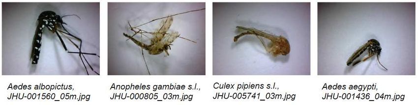
transportation. Addressing the increased complexity of identifying wild-caught mosquito
specimens is essential for developing a practical computer vision solution usable by mosquito
control programs. Mosquito identification can be challenging, with many species of similar
morphology. While some previous work has gone beyond genus-level classification to identify
species, most have tested morphologically dissimilar species20, or pristine specimens readily
available from laboratory colonies21, rather than environmental specimens.

Reliance on laboratory reared specimens aside, all computer vision methods for mosquito
classification to date have been limited to closed-set classification of no more than 17 species.
There are currently 3570 formally described species and 130 subspecies in the 41 genera that
comprise the family Culicidae22, and many new species detected genetically that await formal
descriptions. Given this, a close-to-complete dataset of all mosquitoes is unlikely and any
computer vision solution must be able to recognize when it encounters a species not
represented in the closed-set of species as previously unencountered, rather than forcing
incorrect species assignment: an open set recognition, or novelty detection, problem. The
novelty detection and rejection problem has been addressed in previous computer vision work,
though most successful methods, are applied to non-fine-grained problems represented by
ImageNet23, CIFAR24, and MNIST25 datasets26, such as the generalized ODIN of Hsu et al.27
and multi-task learning for open set recognition of Oza et al28.

Given the fine-grained morphological diversity between closely related mosquito species and
the intra-specific variability (of both form and acquired damage) between wild-caught
specimens, this problem is succinctly defined as a noisy, fine-grained, open set recognition
object classification problem. Defining the problem as such is necessary for practical
implementation, and has not yet been addressed, nor has this type of problem been sufficiently
solved in the wider computer vision literature. Herein, we present a convolutional neural
network-based approach to open set recognition, designed for identifying wild caught mosquito
specimens. When presented with an image, our algorithm first determines whether its species is
known to the system, or is novel. If known, it classifies the specimen as one of the known
species. The novelty detection algorithm was evaluated using 25-fold cross validation over 67
species, and the final classification CNN using 5-fold cross-validation over 20 potentially known
species, using 16 of these species as known for each fold, such that each known species is
considered unknown for one of the five folds of the CNNs. Evaluation included specimens of
species known to the closet-set classification CNN, unknown species which were used to train
the algorithm to detect when a species was novel to the CNN, and novel unknown species
which were not used in training (hereafter referred to as known, unknown, and novel unknown).
All specimens used in the study were expertly identified (by morphology or by DNA barcoding),
thus reference to known or unknown species in this context is indicative of whether the CNN
has prior knowledge of the species presented. We also provide an evaluation of 39 species
closed-set classification and a comparison of our methods to some common alternatives. The
image database developed for training and testing this system consists of primarily wild caught
specimens bearing substantial physical damage, obfuscating some diagnostic characters (see
Figure 1).

 3

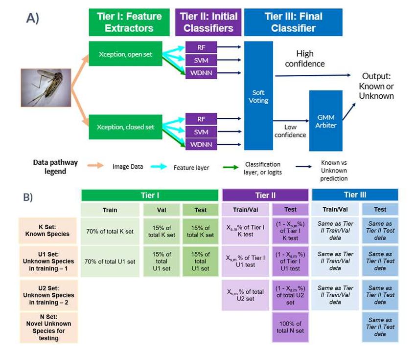
Figure 1. Example image database samples of wild-caught mosquitoes. Field specimens were often
considerably damaged, missing appendages, scales, and hairs, like specimens captured during standard
mosquito surveillance practice.

Results
System Overview
To address the open-set novel species detection problem, our system leverages a two-step
image recognition process. Given an image of a mosquito specimen, the first step uses CNNs to
extract relevant features from the image. The second step is a novelty detection algorithm,
which detects whether the mosquito is a member of one of the sixteen species known to the
CNNs of the system. If the mosquito is not a member of one of the known species, it is
classified as novel, or unknown. This detection algorithm is tested on truly novel mosquito
species, never seen by the system in training, as well as species used in training. If a mosquito
is recognized by the system as belonging to one of the sixteen known species (i.e. not novel),
the image proceeds to species classification with one of the CNNs used to extract features.

Unknown Detection Accuracy
In distinguishing between unknown species and known species, the algorithm achieved an
average accuracy of 89.50±5.63% and 87.71±2.57%, average sensitivity of 92.18±6.34% and
94.09±2.52%, and specificity of 80.79±7.32% and 75.82±4.65%, micro-averaged and macro-
averaged respectively, evaluated over twenty-five-fold validation (Table 1). Here, micro-average
refers to the metric calculated without regard to species, such that each image sample has an
equal weight, considered an image sample level metric. Macro-average refers to the metric first
calculated within a species, then averaged between all species within the relevant class (known
or unknown). Macro-average can be considered a species level metric, or a species normalized
metric. Macro-averages tend to be lower than the micro-averages when species with higher
sample sizes have the highest metrics, whereas micro-averages are lower when species with
lower sample sizes have the highest metrics. Cross validation by mixing up which species were
known and unknown produced variable sample sizes in each iteration, because each species
had a different number of samples in the generated image dataset. Further sample size
variation occurred as a result of addressing class imbalance in the training set. The mean
number of samples varied for each of the twenty-five iterations because of the mix-up in data
partitioning for cross-validation (see Table 1 for generalized metrics; see Supplementary Table
1, Datafolds for detailed sampling data).

Table 1. Micro- and macro-averaged metrics of the novelty detection algorithm on the test set
using fifty-fold validation.
 Known samples Unknown Average Unknown Unknown Unknown
 (avg (min-max)) Samples accuracy sensitivity/ specificity Precision
 (avg (min-max)) recall

 Micro- 519.44 (409- 2216.12 (1043- 89.50± 92.18± 80.79± 94.21±
 average 1 694) 3557) 5.63% 6.34% 7.32% 3.76%

 Macro- 15.8 (15-16) 3 29.84 (25-34) 3 87.71± 94.09± 75.82± 79.66±
 average 2 2.57% 2.52% 4.65% 3.24%

1
 Micro-average refers to the metric calculated without regard to species as an independent class: each sample has an equal weight.
2
 Macro-average refers to the metric calculated first within each species as an independent class, then averaged between species
for the known or unknown classes, in order to address imbalance of samples between species.
3
 This indicated the number of species in the known or unknown classes for each macro-average.

Differences within the unknown species dictated by algorithm structure

 4

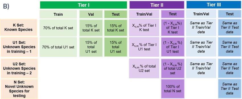
The fundamental aim of novelty detection is to determine if the CNN in question is familiar with
the species, or class, shown in the image. CNNs are designed to identify visually distinguishable
classes, or categories. In our open-set problem, the distinction between known and unknown
species is arbitrary from a visual perspective; it is only a product of the available data. However,
the known or unknown status of a specimen is a determinable product of the feature layer
outputs, or features, produced by the CNN’s visual processing of the image. Thus, we take a
tiered approach, where CNNs trained on a specific set of species extract a specimen’s features,
and independent classifiers trained on a wider set of species analyze the features produced by
the CNNs to assess whether the CNNs are familiar with the species in question. The novelty
detection algorithm consists of three tiers, hereafter referred to as Tier I, II, and III, intended to
determine if the specimen being analyzed is from a closed set of species known to the CNN:
 Tier I: two CNNs used to extract features from the images.
 Tier II: a set of classifiers, such as SVMs, random forests, and neural networks, which
 independently process the features from Tier I CNNs to distinguish a specimen as either
 known or unknown species.
 Tier III: soft voting of the Tier II classifications, with a clustering algorithm, in this case a
 Gaussian Mixture Model (GMM), which is used to make determinations in the case of
 unconfident predictions.

The tiered architecture necessitated partitioning of groups of species between the tiers, and an
overview of the structure is summarized in Figure 2a. The training schema resulted in three
populations of unknown species: set U1, consisting of species used to train Tier I, also made
available for training subsequent Tiers II and III; set U2, consisting of additional species
unknown to the CNNs used to train Tiers II and III; and set N, consisting of species used only for
testing (see Figure 2b). Species known to the CNNs are referred to as set K. It is critical to
measure the difference between these species sets, as any of the species may be encountered
in the wild. U1 achieved 97.85±2.81% micro-averaged accuracy and 97.34±3.52% macro-
averaged accuracy; U2 achieved 97.05±1.94% micro-averaged accuracy and 97.30±1.41%
macro-averaged accuracy; N achieved 80.83±19.91% micro-averaged accuracy and
88.72±5.42% macro-averaged accuracy. The K set achieved 80.79±7.32% micro-averaged
accuracy and 75.83±5.42% macro-averaged accuracy (see Table 2).

 5

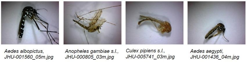
Figure 2. The novelty detection architecture was designed with three tiers to assess whether the
CNNs were familiar with the species shown in each image. A) Tier I consisted of two CNNs used as
feature extractors. Tier II consisted of initial classifiers making an initial determination about whether the
specimen is known or unknown by analyzing the features of one of the Tier I CNNs, and the logits in the
case of the wide and deep neural network (WDNN). In this figure, SVM refers to a support vector
machine, and RF refers to a random forest. Tier III makes the final classification, first with soft voting of
the Tier II outputs, then sending high confidence predictions as the final output and low confidence
predictions to a Gaussian Mixture Model (GMM) to serve as the arbiter for low confidence predictions. B)
Data partitioning for training each component of the architecture is summarized: Tier I is trained on the K
set of species, known to the algorithm; Tier I open-set CNN is also trained on the U1 set of species, the
first set of unknown species used in training; Tier II is trained on K set, U1 set, and the U2 set of species,
the second set of unknown species used in training; Tier III is trained on the same species and data-split
as Tier II. Data-split ratios were variable for each species over each iteration (Xs,m where s represents a
species, m represents a fold, and X is a percentage of the data devoted to training) for Tiers II and III; Xs,m
was adjusted to manage class imbalance within genus across known and unknown classes. Testing was
performed on each of the K, U1, and U2 sets, as well as the N set, the final set of unknown species
reserved for testing the algorithm, such that it is tested on previously unseen taxa, replicating the
plausible scenario to be encountered in deployment of CNNs for species classification. Over the twenty-
five folds, each known species was considered unknown for at least five folds and included as novel for at
least one-fold.

Table 2. Accuracy metrics for the known, unknown, and novel unknown species sets over twenty-
five-fold validation.
 Accuracy, macro- Accuracy, micro- Number of species Number of samples
 average average tested within set (avg within set (avg (min-
 (min-max)) 2 max)) 2

 Set K 1 75.83±4.65% 80.79±7.32% 15.8 (15-16) 519.44 (409-694)

 Set U1 1 97.34±3.52% 97.85±2.81% 8.8 (7-10) 54.04 (44-67)

 Set U2 1 97.30±1.41% 97.05±1.94% 10.28 (6-15) 1612.72 (159-3189)

 Set N 1 88.72±5.42% 80.83±19.91% 10.76 (8-13) 549.36 (96-1193)
1
 Set K species are known to the closed-set CNNs. Set U1 unknown species are used in training for Tiers I, II & III. Set U2 unknown
species are used to train Tier II&III. Set N unknown species are novel to all tiers and reserved for testing.
2
 The extreme variation in the test set was due to class balancing the Tier II&III training data, such that whenever a genus was
represented in the K set a similar number of specimens from that genus were available for the unknown training set, whenever
possible. Some of the U2 species were only used during training due to limited numbers of specimens in particular species.

 6

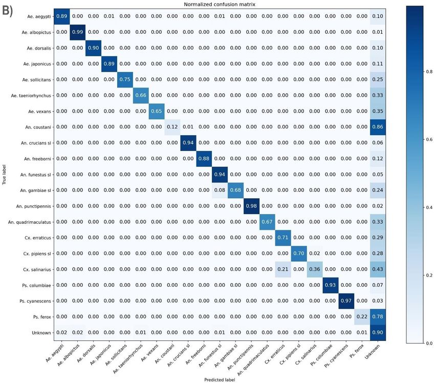
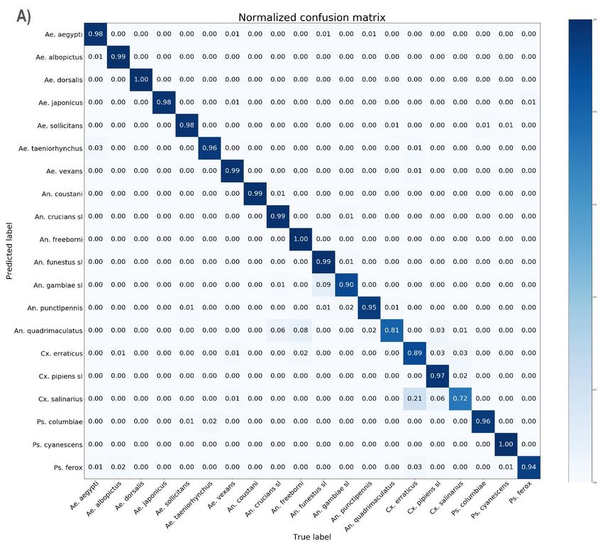
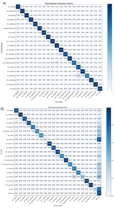
Subsequent Species Classification
Following the novelty detection algorithm, species identified as known are sent for species
classification to the closed-set Xception model used in Tier I of the novelty detection algorithm.
Figure 3a shows the species classification results independently over the five folds of Tier I,
which achieved a micro-averaged accuracy 97.04±0.87% and a macro F1-score of
96.64±0.96%. Figure 3b shows the species classification cascaded with the novelty detection
methods where all unknown species are grouped into a single unknown class alongside the
known classes in an aggregated mean confusion matrix over the twenty-five folds of the full
methods, yielding a micro-averaged accuracy of 89.07±5.58%, and a macro F1-score of
79.74±3.65%. The confusion matrix is normalized by species and shows the average
classification accuracy and error distribution. The independent accuracy for classifying a single
species ranged from 72.44±13.83% (Culex salinarius) to 100±0% (Aedes dorsalis, Psorophora
cyanescens), and 15 of the 20 species maintained an average sensitivity above 95%.

 7

Figure 3. Mean normalized confusion matrices for species classification shows the distribution of
error within species. The species classification in these confusion matrices was performed by the Tier I
CNN, the closed set Xception model. The confusion matrix conveys the ground truth of the sample
horizontally, labels on the left, and the prediction of the full methods vertically, labels on the bottom.
Accurate classification is across the diagonal, where ground truth and prediction match, and all other cells
on the matrix describe the error. Sixteen species were known for a given fold, and 51 species were
considered unknown for a given fold, with each of the twenty known species considered unknown for one
fold. A) The species classification independent of novelty detection shows an average accuracy of
97.04±0.87% and a macro F1-score of 96.64±0.96%, calculated over the five folds of Tier I classifiers,
trained and tested over an average of 7174.8 and 1544.6 samples. Of the error, 73.5% occurred with
species of the same genus as the true species. B) The species classification as a subsequent step after
novelty detection yielded 89.07±5.58% average accuracy, and a macro F1-score of 79.74±3.65% trained
and tested on an average of 7174.8 and 519.44 samples, evaluated over the twenty-five folds of the
novelty detection methods. First, a sample was sent to the novelty detection algorithm. If the sample was
predicted to be known to the species classifier, which was the closed-set Xception algorithm used in Tier
I, then the sample was sent to the algorithm for classification.

Many of the species which were a part of the unknown datasets had enough data to perform
preliminary classification experiments. Thirty-nine of the 67 species had more than 40 image
samples. Species classification on these 39 species yielded an unweighted accuracy of

 8

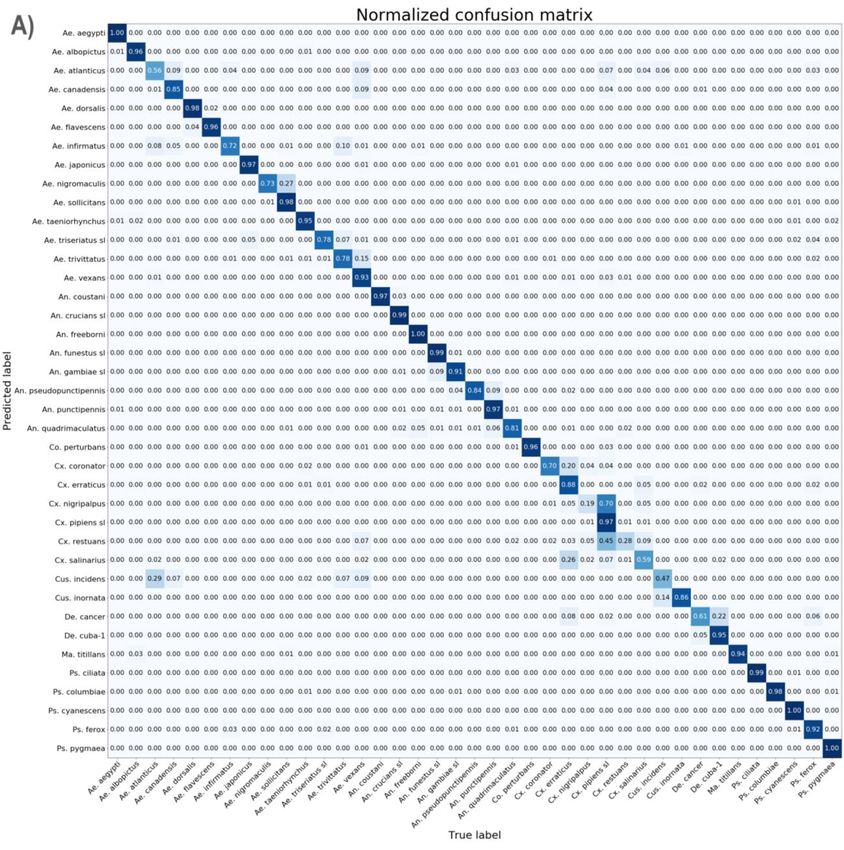
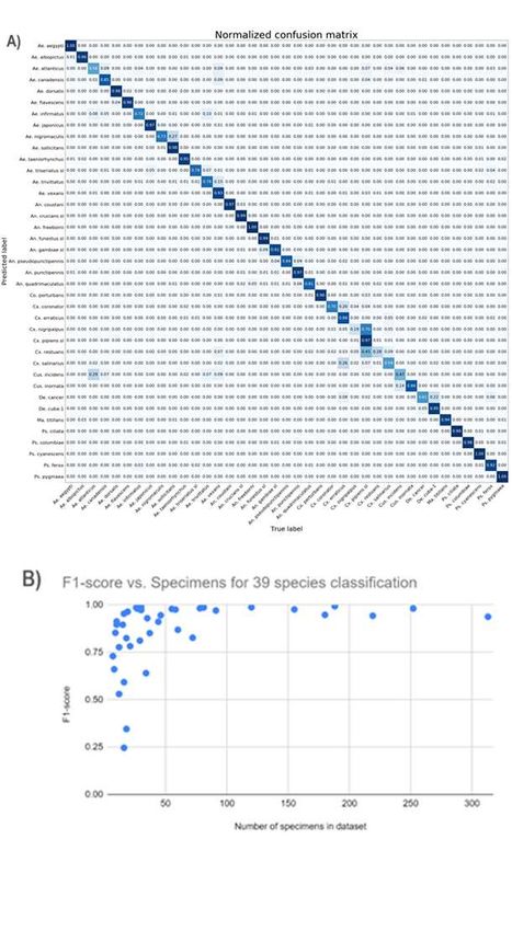
93.06±0.50% and a macro F1-score of 85.07±1.81% (see Figure 4a). The average F1-score for
any one species was plotted against the number of specimens representing the samples in the
species, which elucidates the relationship between the training data available and the accuracy
(see Figure 4b). No species with more than 100 specimens produced an F1-score below 93%.

 9

Figure 4. Species classification across 39 species shows the strength of CNNs for generalized
mosquito classification, and elucidates a guideline for the number of specimens required for
confident classification. Classification achieved unweighted accuracy of 93.06±0.50% and a macro F1-
score of 85.07±1.81%, trained, validated, and tested over an average of 9080, 1945, and 1945 samples
over five folds. A) The majority of the error in this confusion matrix shows confusion between species of
the same genera. Some of the confusion outside of genera is more intuitive from an entomologist
perspective, such as the 10.2% of Deinocerites cancer samples classified as Culex spp. Other errors are
less intuitive, such as the 28.61% of Culiseta incidens samples classified as Aedes atlanticus. B) This plot
of average F1-score of a species against the number of specimens which made up the samples available
for training and testing shows the relationship between the available data for a given specimen and
classification accuracy. When following the database development methods described in this work, a
general guideline of 100 specimens’ worth of data can be extrapolated as a requirement for confident
mosquito species classification.

Comparison to alternative methods
Some intuitive simplifications of our methods, along with some common direct methods for
novel species detection, are compared to our full methods. All compared methods were found to
be statistically different from the full methods using McNemar’s test. The compared methods
tested, along with their macro F1-score, standard deviation, and p-value as compared to the full
methods, were as follows: 1) soft voting of all Tier II component outputs, without a GMM arbiter
(86.87±3.11%, p < 0.00001); 2) the Random Forest Tier II component, appended to the closed
set classification CNN from Tier I (82.80±3.84%, p < 0.00001); 3) the SVM Tier II component,
appended to the closed set classification CNN from Tier I (82.68±4.51%, p < 0.00001); 4) the
WDNN Tier II component, appended to the closed set classification CNN from Tier I
(81.87±4.53%, p < 0.00001); 5) the softmax of the closed-set Xception logits, producing an
unknown prediction for those specimens where no probability exceeded a threshold determined
during training (72.38±4.43%, p < 0.00001); 6) using the predicted class of the open-set
Xception model, but remapping any genus level class and the general mosquito class to the
unknown class (72.72±4.28%, p < 0.00001). Our full novelty detection methods are significantly
different from each alternative method tested on these twenty-five folds, but with macro F1-
score and standard deviation (86.24±2.48%) similar to the simplified methods. The difference is
noticeable in a higher macro-averaged unknown sensitivity for the full methods, seen in Table 3,
the advantages of which are discussed in the discussion.

Table 3. Comparison of our methodology to simpler alternative methods.
 McNemar’s Test, ฀21 Macro F1-score Macro Unknown Recall/ Macro Unknown
 Sensitivity Precision
Full methods 86.24±2.48% 94.09±2.42% 79.66±3.24%
Soft voting of all ฀21 = 332 1 86.87±3.11% 88.55±3.58% 85.36±3.93%

 10

T2 components p < 0.00001
T2 – closed-set 21 = 920
 p < 0.00001
 82.80±3.84% 83.79±4.86% 81.97±4.23%
Random Forest
T2 – closed-set 21 = 1120
 p < 0.00001
 82.68±4.51% 82.93±5.68% 82.58±4.60%
SVM
T2 – closed-set 21 = 905
 p < 0.00001
 81.87±4.53% 87.34±5.96% 77.11±3.93%
WDNN
Softmax with a 21 = 12151
 p < 0.00001
 72.38±4.43% 61.81±4.31% 87.43±5.47%
threshold
Open-set re- 21 = 24656
 p < 0.00001
 72.72±4.28% 58.03±5.52% 98.02±1.98%
mapped
1
 A high chi-squared ( 21) value dictates a low p-value, which indicates a statistically significant difference with the full methods.

Discussion
The novelty detection algorithm presented achieves an accuracy of 89.50±5.63% in identifying
unknown species using field mosquito specimens, outperforming other common methods in
terms of unknown sensitivity and F1-score. Cascaded with closed-set classification, the overall
classification accuracy is 89.07±5.58%. Closed-set classification on 16 known species achieves
97.04±0.87% accuracy and a macro F1-score of 96.64±0.96%. A widened closed set of 39
species classification achieves 93.06±0.50% accuracy and a macro F1-score of 85.07±1.81%.
This work represents two landmarks in the field of computer vision-based mosquito recognition:
1) the use of wild caught specimens with highly variable physical condition for classification
across a wide set of species, including morphologically similar species; and 2) accurate
detection of species novel to the classification algorithm, such that practical deployment need
not be limited to regions where all mosquito species are included in the database. The high
accuracy species classification paired with novel species detection validates the practical use of
computer vision for mosquito identification and demonstrates its potential as a reliable
identification method even between species of similar morphology. Most important, the
introduction of a novelty detection algorithm tested on species of similar morphology to those in
the known species distribution offers a practical path to deployment of these algorithms in the
field in the face of otherwise impractical database requirements, to supplement and fill gaps in
current vector surveillance programs globally. In short, we have demonstrated a viable
computer vision solution to the noisy, fine-grained, open-set classification problem of mosquito
species identification.

A major roadblock to developing a field ready machine learning-based mosquito identification
algorithm is amassing a database sufficient to recognize any one of the over 3500 mosquito
species. This is difficult not only due to the distribution of these species around the world, but
also the difficulty of capturing many of these species, and of taxonomists' ability to recognize
them, as most taxonomists only learn the species of a region relevant to their work. By
introducing the unknown category, we can focus on training algorithms to identify common and
medically relevant species, with confidence that species outside of our dataset will be
categorized as an unknown species. Furthermore, classification with 39 species of limited data
shows that species with more than 100 specimens produce confident classifications above 90%.
Though some species may be more distinct than others, enabling high accuracy with smaller
datasets, 100 specimens may be used as a guideline for data requirements for mosquito
species classification with computer vision, until more thorough research on this question has
been done. This work defines and dramatically reduces the data necessary for mosquito
classification with computer vision as a useable tool, clarifying a viable path forward for practical
use by vector control organizations for disease prevention.

 11

Although the overall accuracy of the 16 species classification is high (97.04±0.87%),
performance was markedly lower for certain species. However, 73.5% of the error occurred
within the genus of the sample. Though the error for identifying Culex salinarius was high, with
20.6% of samples confused with Culex erraticus and 6.1% confused with Culex pipiens sl,
similar error within a genus is also more common among human experts, particularly within
Culex. The authors attribute the error which lies outside genera to three compounding factors:
1) the limited amount of data available, given that 97% of the species normalized error that
occurred outside of genus involved species with fewer than 100 specimens; 2) the stochastic
nature of training deep neural networks, which in the face of limited data may produce
unexpected error distribution; 3) and the highly damage nature of many of the specimens in the
image database produced for this work, which may also be minimized by increasing training
dataset size. Future work should investigate novelty detection as a broader application of
distinguishing both novel species and low confidence specimens from closed-set classifications.
Furthermore, other variables could be distinguished alongside species identification, such as
mosquito sex, age, and feeding state. Analysis of these attributes may impact species
identification accuracy, as well as provide additional value to mosquito control organizations.
Given the diversity of species in different regions, inclusion of geographical and temporal
information for time and place of capture may improve classification accuracy, as was recently
done for butterfly classification29, another fine grained insect classification problem.

The novel, or unknown, species detection method in this work is important both to mosquito
identification and to the field of computer vision. Previous work in recognizing novel classes,
such as Outlier detection in neural networks (ODIN) and others described in the review by Geng
et al. on open set recognition methods, has been focused on novel classes far outside the
distribution of known classes27. However, these algorithms do not perform well on extremely
fine-grained tasks, such as that presented in this work. Closed-set computer vision algorithms,
such as those presented in previous works on mosquito classification, can only classify species
on which they have been trained. This is similar to current entomological practice which relies
on dichotomous keys that typically only contain a select group of species common to a
particular region. If a mosquito belongs to a species not in the key, a technician will either
mistakenly label it as a species they know, or they will recognize the anomaly and set the
specimen aside for further analysis. Accurately identifying unknown species is a challenging
problem because there is no visual or morphological reason for the distinction; it is an artificial
product of what the user, or algorithm, is familiar with. Since a species’ unknown status is not
necessarily indicative of visual characteristics far distinguished from the known species, the
differences may not be an abstraction of the images themselves, but an abstraction of the
features generated by a CNN processing the image in attempting species classification. This
theory is the basis for the tiered approach of the novelty detection algorithm as presented in this
work, where the features are analyzed by tiers of classifiers which are trained after the initial
training of the CNNs. Disjointing the learning of feature extraction from the novelty detection
portions of the methods and isolating feature extraction learning to species classification
enables the later tiers to be independent arbiters of the novelty of the species in question.
Future work should attempt to improve upon these methods, testing them on to similar many-
class fine-grained classification problems with inherent class imbalance issues.

The markedly lower performance of N set as compared to U1 set and U2 set is expected given
that the CNNs did not train on the N set species. The difference between the micro-averaged
and macro-averaged accuracies of N set (80.83±19.91% and 88.72±5.42%) indicates that the
species within N set which contain the most specimens also tend to be the species most distinct
from the K set, despite species mix-up with cross-validation. However, it is notable that the U2

 12

set species achieved high micro-averaged and macro-averaged accuracies (97.05±1.94% and
97.30±1.41%). Many of the U2 species contained only a few samples. This suggests that if only
a few specimens are obtained from otherwise unknown species, the species can be included in
U2, and thereafter provide little threat of error regarding our unknown algorithms. The novelty
detection accuracy for the K set known species was lowest of the species sets (80.79±7.32%
micro-averaged and 75.83±4.65% macro-averaged). Though some of the compared novelty
detection methods exceeded the full methods in known recall, or known sensitivity, the full
methods are preferable from an entomologist perspective because they bias answers towards
unknown. Mosquito taxonomists are conventionally trained to only provide confident answers.
For example, if they think a specimen in question may be Culex erraticus but they are unsure,
they are encouraged to call the specimen Culex spp. if they are confident of the genus, or to
family Culicidae if they are not. In this way, the full methods, and in particular the inclusion of the
GMM arbiter in Tier III, are preferable to the simpler alternatives, as they bias answers towards
unknown, rather than known.

A potential application of this technology is in the recognition of malaria vectors. A major
challenge to malaria elimination is weak surveillance, monitoring, and evaluation 30. Although
long-lasting insecticide nets and indoor residual spraying efforts have yielded progress, malaria
elimination has been set back in many countries by insecticide resistance, the misuse of
interventions, host behavior (such as cooking outdoors in the early evening) and adaptive vector
behavior (such as biting earlier in the evening, before humans are under the protective cover of
bed nets). In sub-Saharan Africa, the primary malaria vectors are Anopheles gambiae s.l. and
Anopheles funestus s.l.; species complexes that are often difficult to distinguish from each other
and other Anopheles species. Ideally, public health systems should know the density,
composition, and distribution of the mosquito species in a finite region, allowing them to
optimize interventions to a particular area3. If an affordable computer vision system were to be
deployed in the field, organizations without access to specially trained taxonomists could obtain
these composition and distribution patterns in a more standardized and timely manner.

The implications of this work for the prevention of mosquito borne diseases are vast. The first
step towards implementing an effective control program is obtaining high quality data on the
disease vectors in an area4,31. Without robust vector surveillance, emerging vector-borne
disease threats cannot be addressed. Current global vector surveillance systems are
unstandardized, burdensome on public health systems, and threatened by the global paucity of
entomologists. Such a computer vision system could empower non-experts to accurately and
rapidly identify disease vectors in the field, increasing programmatic capability and capacity with
minimal training and cost.

Methods

Image database development
A diverse database of mosquito images was developed primarily from desiccated mosquito
specimens from field sites across Africa and North America, but was supplemented by lab
colony specimens from species for which field specimens were difficult to obtain. Specimens
ranged in condition from fully intact to missing appendages with badly damaged head and/or
body (see Supplementary Figure 1, Image Database Preview). Each mosquito was identified by
either genetic identification or human expert identification under a microscope. Expert
identification was only used when genetic identification was unavailable, or the mosquito was
grown in a lab colony. The molecular identification approach used was DNA-barcoding
performed by Walter Reed Biosystematics Unit (WRBU), where DNA signatures are compared
against the gold-standard Mosquito Barcoding Initiative reference libraries32–34, or identified

 13

using specific nuclear DNA ITS2 assays where available35,36. All DNA barcodes generated for
mosquitoes imaged in this study are publicly available through GenBank, under accession
numbers XXX-XXX [to be added at stage of proof]. Associated data and raw chromatograms
are hosted on the Barcode of Life Database (BOLD; www.boldsystems.org), under the container
JHUSM and project codes SMARU, SMARV, SMARW and SMARX. Each mosquito was
imaged at multiple random orientations on a white background, resulting in 4-10 images per
mosquito. By this process, 12,977 photos of 2,696 specimens from 67 species were generated,
(see Supplementary Table 2, Image Database Details). Of the 2696 specimens, 53.1% were
identified using DNA and 86.4% were wild caught, and of the 67 species, 95.5% consisted
solely of wild-caught specimens.

Specimens were photographed with a handheld, USB microscope (Zarbeco MiScope Handheld
Digital Microscope - MiSC-s2) set at 40X zoom, producing images of 640x480 pixels. The
resolution of the microscope at 40X zoom was measured at 28 line pairs/millimeter, or 18
resolvable microns, characterized using the United States Air Force 1951 Resolution Chart.
During training, images were made square by adding a patch of background color to the top and
bottom of each image, by taking the mean of each channel for the top 5 and bottom 5 rows of
the image. After being made square, the images were down sampled to 299x299 pixels before
being fed to the CNNs to match the image size of the selected architecture. Of the 67 species,
20 species were selected to be considered known based on the number of specimens in the
database, the species’ medical relevance, and addressing class balance between known and
unknown. For each of the five data folds, 4 of the 20 known species were removed to the
unknown category, leaving 16 known species for each fold. Each species was considered
unknown for one of the five folds. To maximize the potential of the limited dataset, we used real
time data augmentation, using the default parameters of the get_transforms function in the
FastAI PyTorch library37 (random cropping, affine transform, symmetric warp, rotation, zoom,
brightness, and contrast modifications with the exception of the affine transform, for which a
dihedral affine was used).

Novelty detection algorithm structure
The three tiers of the novelty detection algorithm are trained independently in sequence.
Different data is used to train Tier I than is used to train Tiers II and III, so that Tiers II and III
can assess the familiarity of Tier I CNNs with the new data presented it, rather than training the
later tiers on data to which Tier I was fit during its training.

Tier I uses two CNNs trained independently on the same data. The models trained were both
Xception38 models, but were trained on different data with different class divisions. The two
datasets were open-set and closed-set, where the closed set model contained only 16 known
species-level classes, and the open set model contained the 16 known species-level classes as
well as 4 genus-level classes and a general mosquito class. The genus-level classes are simply
formed of groups of species of the same genus and do not include any specimens of the 16
known species. The mosquito class consists of multiple genera outside the genera described by
the other 20 classes. The CNNs were trained with a fully connected classification head, the
open-set Xception with 21 nodes and the closed-set Xception with 16 nodes. For Tier I, in the
training of Xception38 models we use a learning rate of 1e-2, with one cycle schedule39. Models
are trained for 60 epochs with Ranger optimizer40 with a batch size of 16. We use categorical
Focal Loss41 with the gamma parameter set to 2. Model training is performed on an RTX 2070
Super GPUs using the deep learning framework PyTorch42.

Tier II consists of three standard machine learning classifiers, a support vector machine (SVM),
a random forest (RF), and a wide and deep neural network (WDNN)43, appended to each the

 14

Tier I CNNs, resulting in six Tier II components. Each attempted to determine whether the given
specimen was from a known species or an unknown species by analyzing the features of the
Tier I CNN, and for the WDNN, both the features and the logits. The SVM uses a Radial-basis
function (RBF) kernel, with a kernel coefficient (γ) set according to γ = 1/(nfeatures * Xvar), where
nfeatures is the number of features per sample and the Xvar is the variance of all samples in the
set44. It derives a squared L2 penalty based on a regularization constant (C) set to 0.1. The RF
fits 200 decision trees with a maximum depth of 19, considering log2(nfeatures) features per split
and using entropy as a measure of impurity44. The WDNN is a deep neural network with two
input layers, a deep input which learns lower dimensional dense representations of the data and
a wide input which memorizes shallow features to help protect the network from over-
generalization. The deep input takes the features (2048 nodes) and passes them to four hidden
layers (2500, 1900, 1900, and 1900 nodes). It uses He normal initialization45 , and includes a
0.65 dropout layer46, a batch normalization layer47, and an ELU activation48 between each
hidden layer. The wide input receives the logits (21 for open-set Xception and 16 for closed-set
Xception) and directly concatenates them with the final hidden layer of the deep network. This
concatenated layer feeds to a single output node to determine known or unknown. The network
is trained for 20 epochs using a binary cross entropy loss function with an Adam optimizer 49.
The learning rate was initially set to 1e-3, decaying every 10 epochs at a rate of 0.1.

Tier III first intakes the unknown probabilities from the six Tier II components and uses soft
voting for the initial assessment (i.e. averaging the six probabilities). Average probabilities, pavg,
are then sorted into confident and unconfident predictions, based on thresholds determined
during training. Unconfident predictions are those where Tknown < pavg < Tunknown, where Tunknown =
0.9, above which an unknown prediction is considered confident, and where Tknown = 0.3, below
which a known prediction is considered confident. Unconfident predictions, where the average
probability falls between the two thresholds, are concluded by evaluating the six tier II
probability scores, p, with a Gaussian Mixture Model (GMM) in sckitlearn44. The GMM performs
unsupervised clustering of known samples, treating unknown samples as anomalies. It fits the
probabilities from the six Tier II components into seven clusters, using a random 10% of the
unknown training data for Tier II/III and all of the known training data. We estimate the density of
the model for each sample using the score_samples method, which finds the log of the
probability density function at that location. The lower the score, the lower the density and the
less likely that the given sample is in the known set. This density is used to measure the
likelihood that a datapoint fits into any of the seven clusters in the model, and the lowest 10% of
these are considered anomalous, or in this case unknown. The 10th percentile defines a density
threshold, below which a sample is determined to be unknown.

Hyper parameter optimization for Tier II and III components was conducted on the training data
for seed 0 of fold 1 using a random search.

Data partitioning and training
Training of the novelty detection algorithm to recognize when a specimen’s species is known or
unknown to the closed-set CNN from Tier I results in three distinct types of data to be
encountered in the wild: specimens from known species recognized by the closed-set CNN (K);
specimens from unknown species used to train the algorithm (U); and specimens from novel
unknown species which were not used in training (N). We evaluate the algorithm on
representations of each of these populations, which we refer to as species sets K, U, and N.

Sixty-seven mosquito species were included in the overall dataset. Twenty of these species
were included in the K dataset. All other species were always used in either the U or N datasets.
Each specimen had multiple photos, and each photo was considered a single sample. When a

 15

specimen was designated for training, validation, or testing for a particular fold, all photos of that
specimen were isolated to that activity.

Tier I closed-set CNNs were trained only on K species. Tier I open-set CNNs were trained on K
species and a subset of U species (U1). The Tier II and III classifiers were trained on K species,
U1 species, and the remaining subset of U species (U2). The remaining set of unknown species
not used in training comprised the novel species testing set N. These species sets are further
described as those used as inputs to Tiers I, II, and III (population represented by group U1),
those used as inputs to train Tiers II and III (population represented by group U2), and those
species which are novel to the algorithm (population represented by group N).

The algorithm training and evaluation was iterated on multiple data splits, assessing different
divisions of species across sets K, U1, U2, and N. In each of the five folds, 4 of the 20 species
considered known were removed from the K set for cross validation, leaving 16 species within
the K set for each fold. U1 species set, a subset of 18 unknown species for training the open-set
Tier I CNN, also trained on by the Tier II and III components, remained the same species for all
folds and iterations, throughout training and testing. The remaining unknown species were
distributed between U2 and N sets. Tier I was iterated on five distinct folds with data from sets K
and U1 using a training:validation:testing split ratio of 70:15:15.

Tier II and III components were trained using the testing data of Tier I. The data split was
iterated 5 times for each of these five folds with data from sets K, U1 and U2, resulting in
twenty-five iterations. For each fold and iteration, the specimens within each set designated for
training and testing were randomized. For each iteration, the unknown species which were
designated for N versus U2 were iterated, being sure that each species was included in the N
set for at least one iteration, except U1 species which could not be iterated in this way. For each
iteration, the percentage of specimens within each species to be designated for training or
testing was first set by a training:testing split ratio of 80:20, then manipulated to reduce class
imbalance between known and unknown within a genus and between morphologically similar
species (see Supplementary Table 1, Datafolds).

Species classification
After the novelty detection methods, if a sample was considered known, the sample was sent to
be classified by the Tier I closed-set CNN. The results are first calculated independent of the
novelty detection methods, including all samples of the species in question which were not
included in training or validation for the training of that fold. Because each fold removed four
species from the dataset, such that each species was considered unknown for one of the five
folds, there was an imbalanced number of iterations distributed across the confusion matrix,
thus each cell is averaged independently. The results are then calculated as a subsequent step
after the novelty detection methods, only classifying species on samples first determined to be
known, and where unknown is maintained as a class within the confusion matrix. This confusion
matrix was calculated over the twenty-five folds of the novelty detection methods, using the
respective Tier I CNN for that fold. Both confusion matrices are normalized. Of the species used
for 16 species closed set classification, test set sample size for each species were as follows
(formatted as species, [fold1,fold2,fold3,fold4,fold5]): Ae. aegypti: [127,0,133,132,126]; Ae.
albopictus: [103,90,0,99,102]; Ae. dorsalis: [43,41,42,0,41]; Ae. japonicus: [162,159,154,156,0];
Ae. sollicitans: [57,0,60,58,60]; Ae. taeniorhynchus: [0,25,27,25,24]; Ae. vexans:
[50,48,0,46,49]; An. coustani: [29,21,18,0,22]; An. crucians s.l.: [56,58,61,61,0]; An. freeborni:
[87,0,77,79,80]; An. funestus s.l.: [158, 174,0,173,175]; An. gambiae s.l.: [182,178,178,0,166];
An. punctipennis: [0,36,31,34,33]; An. quadrimaculatus: [0,28,28,28,30]; Cx. erraticus:

 16

[47,47,44,49,0]; Cx. pipiens s.l.: [212,0,218,219,205]; Cx. salinarius: [25,26,0,26,25]; Ps.
columbiae: [66,59,67,0, 64]; Ps. cyanescens: [0,55,56,54,56]; Ps. ferox: [40,31,41,34,0].

Of the 67 species recorded in our dataset, 39 of them have more than 40 photos, and were thus
included in the widened closed-set species classification, which was trained over five data folds
on the same architecture and hyper parameters stated for training the Tier I closed-set CNN.
The five data folds simply iterated the distribution of specimens across the training : validation :
testing split. The average macro-F1-score and average accuracy, and their standard deviations
over the five folds were reported, along with an average normalized confusion matrix, and a
graph comparing the average accuracies to the number of specimens in the database. Of the
species used for 39 species closed set classification, test set sample size for each species were
as follows (formatted as species, [fold1,fold2,fold3,fold4, fold5]): Ae. aegypti:
[131,127,127,124,133]; Ae. albopictus: [99,99,107,97,95]; Ae. atlanticus: [15,13,14,14,15]; Ae.
canadensis: [17,21,21,21,20]; Ae. dorsalis: [42,41,43,40,43]; Ae. flavescens: [13,14,14,14,14];
Ae. infirmatus: [17,15,19,18,16]; Ae. japonicus: [155,153,151,160,150]; Ae. nigromaculis:
[6,6,5,5,5]; Ae. sollicitans: [63,61,58,57,60]; Ae. taeniorhynchus: [30,25,27,25,25]; Ae. triseriatus
s.l.: [14,16,17,14,13]; Ae. trivittatus: [28,24,25,24,23]; Ae. vexans: [46,58,57,51,50]; An.
coustani: [25,32,27,33,27]; An. crucians s.l.: [64,57,60,59,62]; An. freeborni s.l.:
[85,77,82,74,89]; An. funestus s.l.: [181,187,166,175,161]; An. gambiae s.l.:
[191,182,178,185,194]; An. pseudopunctipennis: [10,8,12,9,9]; An. punctipennis:
[32,28,38,32,32]; An. quadrimaculatus: [30,33,26,37,35]; Coquillettidia perturbans:
[31,29,30,32,35]; Cx. coronator: [10,9,10,11,10]; Cx. erraticus: [48,51,49,53,50]; Cx. nigripalpus:
[14,14,13,13,13]; Cx. pipiens s.l.: [205,203,216,208,216]; Cx. restuans: [12,13,12,14,12]; Cx.
salinarius: [24,25,24,23,24]; Cus. incidens: [9,9,9,9,8]; Cus. inornata: [9,9,8,9,9]; Deinocerites
cancer: [10,10,10,10,9]; De. sp. Cuba-1: [16,14,15,14,15]; Mansonia titillans: [15,16,15,14,13];
Ps. ciliata: [29,26,24,23,28]; Ps. columbiae: [62,59,63,60,61]; Ps. cyanescens: [55,54,57,55,55];
Ps. ferox: [32,48,31,36,34]; Ps. pygmaea: [24,25,25,24,25].

Analysis methodology of detecting novel species
For each of the fifty iterations, the algorithm’s performance on both known and unknown species
was evaluated. The accuracy, unknown sensitivity/recall, unknown specificity, and unknown
precision was calculated for each iteration, and mean and standard deviation of each species
set (K, U1, U2, and N) was reported. Micro-average results are reported considering each
sample with an equal weight, and macro-average results are reported considering the mean for
each species with an equal weight. A mean confusion matrix was calculated using closed-set
Xception model results for the five folds. The 20 known species were considered as distinct
classes, and the remaining species grouped together as a distinct unknown class. Each of the
twenty-five iterations of Tier II and III was cascaded within its respective fold of the five folds of
Tier I to calculate the unknown detection and species classification confusion matrix. The test
set sample sizes for each of the twenty five folds are as follows, (formatted [K-taxa, K-samples,
U1-taxa, U1-samples, U2-taxa, U2-samples, N-taxa, N-samples]): [16,683,8,51,10,536,13,456],
[16,673,8,51,9,537,13,485], [16,673,8,51,8,523,13,508], [16,673, 8,46,6,159,11,869],
[16,694,8,51,7,483,10,548], [15,409,9,62,11,2906,8,546], [15,456,9,62,9,2458,12,1024],
[15,456,10,67,13,2359,9,1115], [15,456,9,62,8,3189,12,306], [15,456,10,67,10,2874,10,601],
[16,543,10,56,12,1450,10,1052], [16,484,9,52,11,2141,10,312], [16,492,10,54,11,2185,12,263],
[16,512,8,45,15,2292,10,189], [16,480,9,49,9,1652,13,790], [16,442,9,44,11,1253,11,665],
[16,494,10,54,14,1727,10,228], [16,442,9,55,13,1803,10,96], [16,538,10,60,8,1509,9,502],
[16,489,10,60,13,1764,9,184], [16,462,8,47,13,1415,11,452], [16,437,8,54,9,1548,11,320],
[16,447,8,55,11,654,10,1193], [16,547,8,44,9,1437,11,531], [16,548,7,52,7,1464,11,499].

 17

In addition, simpler methods for novelty detection were compared to our methods to assess the
need for the complexity of our novelty detection algorithm (see Table 3). The simpler methods
are as follows: our full methods without the GMM arbiter for low confidence samples, such that
the final prediction is made by soft voting; the Tier II RF component appended to the Tier I
closed-set CNN; the Tier II WDNN component appended to the Tier I closed-set CNN; the Tier II
SVM component appended to the Tier I closed-set CNN; the Tier I open-set CNN, where any of
the five open-set classes are considered unknown classifications; a softmax applied to the logits
of the Tier I closed-set CNN, where unknown classification is given if no species receives a
probability higher than a threshold determined through evaluation on the training set (0.99).
McNemar’s Test50 was used to compare the accuracies between each alternative method and
our methods to assess discordance. These comparisons were performed on the same data
folds, so the comparison was paired. The known and unknown precision and recall were also
reported for each method.

Statistics
The accuracy metrics used throughout this work were accuracy, precision, recall (equivalent to
sensitivity), specificity, and F1-score:
 ∗ 
 1 = 2 ∗ Equation 1.
 + 

Macro F1-score is determined by calculating the F1-score for each species, then averaging the
F1-score across species. This controls for class imbalance in the test set. For fold 2, all samples
for An. quadrimaculatus were used in training the known set, so for cascading the unknown
detection with closed-set classification the F1-score for this species was omitted, as there was
no possibility for true positives by which to calculate it. The error bars were calculated using
sample standard deviation:

 ∑( − )2
 = √ Equation 2.
 −1

where sx is the standard deviation, xi is a given sample of measurement, is the average of the
sample population in question, and n is the number of samples. When comparing the difference
between methods, given that the testing and training data was paired through all folds and
iterations, McNemar’s Test with continuity correction was used to assess significance:

 (| − |−1)2
 21 = Equation 3.
 + 

where b is the number of samples where our method was correct and the alternative method in
question was incorrect, c is the number of samples where the alternative method in question
was correct and our method was incorrect, and 21 is the test statistic with a chi-squared
distribution and 1 degree of freedom.

Data Availability
The datasets generated during and analyzed during the current study are available from the
corresponding author upon reasonable request.

Code Availability
The code used to generate the results in this study are available in the GitHub repository:
https://github.com/vectech-dev/novel-species-detection.

 18