Welfare and the depth of informality - Evidence from five African countries WIDER Working Paper 2021/25
←
→
Page content transcription
If your browser does not render page correctly, please read the page content below

WIDER Working Paper 2021/25

Welfare and the depth of informality

Evidence from five African countries

Eva-Maria Egger1, Cecilia Poggi2, and Héctor Rufrancos3

February 2021
Abstract: This study explores the relationship between household poverty and depth of
informality by proposing a new measure of informality at the household level. It is defined as the
share of activities (hours worked or income earned) without social insurance for wage workers in
the household. We apply cross-sectional regressions to five urban sub-Saharan African countries,
showing that a household head informality dummy obscures a non-linear relationship between the
depth of household informality and welfare outcomes. In some countries, a small share of income
from formal jobs is associated with at least the same welfare as a fully formal portfolio. By assessing
transitions between household portfolios with panel data for urban Nigeria, we also show that
most welfare differences are explained by selection and that movements in and out of formality
cannot sufficiently change welfare trajectories. The results call for better inclusion of informal
profiles to social insurance programmes.
Key words: informality, measurement, poverty, social protection, sub-Saharan Africa
JEL classification: H55, I31, J46, J88
Acknowledgements: We would like to thank Kalle Hirvonen, the seminar participants at IFPRI
Ethiopia, the EU-AFD Research Facility on Inequality event at Addis Ababa University, and the
participants at the UNU-WIDER workshop on Transforming Informal Work and Livelihoods for
useful comments. This paper solely expresses the views of the authors and does not reflect the
official position of AFD, UNU-WIDER, or other institutions.

1   UNU-WIDER, corresponding author: egger@wider.unu.edu; 2 Agence Française de Développement (AFD), Paris, France;
3   University of Stirling/Global Labor Organization, Stirling, Scotland, UK
This study has been prepared within the UNU-WIDER project Transforming informal work and livelihoods.
Copyright © UNU-WIDER 2021
UNU-WIDER employs a fair use policy for reasonable reproduction of UNU-WIDER copyrighted content—such as the
reproduction of a table or a figure, and/or text not exceeding 400 words—with due acknowledgement of the original source,
without requiring explicit permission from the copyright holder.
Information and requests: publications@wider.unu.edu
ISSN 1798-7237 ISBN 978-92-9256-963-1
https://doi.org/10.35188/UNU-WIDER/2021/963-1
Typescript prepared by Mary Lukkonen.
United Nations University World Institute for Development Economics Research provides economic analysis and policy advice
with the aim of promoting sustainable and equitable development. The Institute began operations in 1985 in Helsinki, Finland, as
the first research and training centre of the United Nations University. Today it is a unique blend of think tank, research institute,
and UN agency—providing a range of services from policy advice to governments as well as freely available original research.
The Institute is funded through income from an endowment fund with additional contributions to its work programme from
Finland, Sweden, and the United Kingdom as well as earmarked contributions for specific projects from a variety of donors.
Katajanokanlaituri 6 B, 00160 Helsinki, Finland
The views expressed in this paper are those of the author(s), and do not necessarily reflect the views of the Institute or the United
Nations University, nor the programme/project donors.
1       Introduction

Informality is associated with risks, such as a lack of insurance against shocks, and therefore directly
related to vulnerability to poverty. The dearth of protective measures in case of need either directly pulls
people into poverty or keeps them poor by changing their behaviour to less risky and less profitable
activities (Dercon 2002). An important risk-coping strategy for households is resource sharing so that
the very trait of informality or related social protection coverage should not be considered solely for the
individual but instead at the household level.

The measurement of informality is not straightforward, nor is information collected in a comparable
manner that would allow for the same definition for different economic agents. For instance, at the
individual level, standard definitions identify informality through the characteristics of the employment
relationship in terms of access to health insurance or pension. At the firm level, the term implies gen-
erally an enterprise lacking a formal registration of its status or a contract with its workforce. At the
household level, for simplicity of comparability, informality is reflected in the status of the household
head’s main occupation. However, the information of the household head alone does not sufficiently
inform any anti-poverty policy (Brown and van de Walle 2020). The departing point of this study is the
observation that empirical studies only consider the formality status of either an individual worker or a
firm, sometimes both, but do not investigate the composition of formality statuses within a household
and associated economic outcomes.

In this article we propose a continuous measure of depth of informality at the household level, defined
either as the share of income from or share of labor input in informal activities, and we investigate
how such informality portfolios relate to household welfare in low-income settings. At the global level,
there exists an inverse U-shaped relationship between economic development and informality (Elgin and
Birinci 2016). However, a reduction in informality at the country level is not always associated with a
reduction in poverty (OECD and ILO 2019). Danquah et al. (2019) find income gains for individuals
moving into formal employment. The present study therefore aims to shed light on this relationship at
the household level by assuming that under income pooling, access to social protection via formal wage
employment of some household members could improve overall household welfare.

The article first estimates in a cross-sectional analysis how household consumption or poverty is related
to the depth of informality in five low-income countries. The data used are the nationally representative
Living Standards Measurement Study—Integrated Surveys on Agriculture (LSMS-ISA) from Ethiopia,
Malawi, Niger, Nigeria, and Tanzania. All countries have both sizeable informal sector participation
and some form of social protection that, albeit fragmented, is an option to some occupational arrange-
ments within and outside of public sector wage employment. We therefore focus on formality by wage
employment and associated coverage of contributory schemes, such as health insurance or pension cov-
erage, and do not inspect the comparative advantage to be or switch across wage and self-employment
[see, for instance, Central America Alaniz et al. (2020)]. In a second step, we present results of a dy-
namic analysis for Nigeria testing the role of transitions between different states of informality portfolios
for household welfare. We report the results solely for urban areas to reduce, at a maximum, possible
confounding factors of wage employment availability. Building upon the labour economics literature
that inspects the characterization of participation into activities (like unionization or contracting), we
compare changes in the employment composition (between fully formal, mixed, and fully informal) in
a traditional dynamic setting between status ‘switchers’ versus ‘stayers’ in the same portfolio as, for
example, Bertrand et al. (2004). To overcome remaining concerns of selection bias, we apply a double
difference strategy of early and late switchers, as proposed by Goodman-Bacon (2018).

The results provide four main insights. First, the depth of informality measured by income and by
labor input shares (in the form of full-time equivalents) present similar results. Thus, our measure can

                                                     1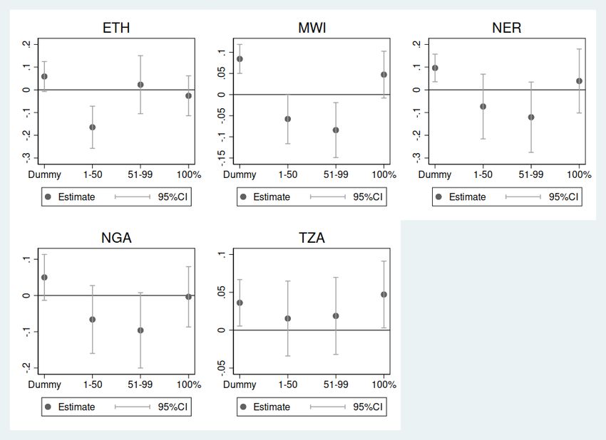
be applied also in settings where only one of the two is possible to construct. Second, the welfare
penalty for an informal household head is directly comparable with that of fully informal households
as defined with our measure. Third, households with a mix of formal and informal income sources
or activities show better welfare outcomes than fully formal households in some countries, or at least
they are not worse off than fully formal ones and always better off than fully informal ones. It appears
that households with a formally employed member fare even better if the household diversifies with
additional income from informal activities. In some countries, an income or activity share in formal
activities of less than half can already make the household relatively better off than a fully informal
employment portfolio. Thus, the informal household head dummy obscures such income diversification
effects. Fourth, our dynamic panel analysis suggests that the cross-sectional gap that we observed is
almost entirely explained by the selection of households transitioning between statuses rather than by
the final outcome of greater informality experienced. There is no evidence of a real gain in changing
from a fully informal status to greater formality of the wage employment composition of a household
portfolio. This gain does not materialize unless there is an underlying selection process that makes
the material gain become massive in terms of consumption. Such a finding thus portrays the fact that
employment spells in and out of informality may not be enough to change the well-being trajectory of
a household, adding to the literature that analyses the relevance for poverty reduction of formalization
into forms of wage employment. Applying a randomization inference (Young 2018), we confirm that
our panel results are not caused by small sample sizes.

This article talks to a set of distinct literature. First, it speaks to the development literature that stud-
ies household well-being and the role of income pooling (Dercon 2002; Attanasio and Lechene 2002;
De Weerdt and Dercon 2006). If informality is considered, it is often solely through binary classifica-
tion. This article takes a more nuanced approach, and we find that a binary indicator for informality does
not adequately capture the welfare nuances experienced by a household as a result of the composition
of their employment portfolio. The second literature studies employment transitions [see, for example,
Danquah et al. (2019); Maloney (1999); Gong et al. (2004)]. Our approach uses the lens of a household
utility framework and thus contributes to our understanding about how changes in formality status are
relevant to overall welfare (or vulnerability level) experienced not only by those people transitioning but
by the whole household. Methodologically, we also inspect and explain why the choice of comparison
groups matters to model the employment portfolio transitions. As a possible practise for analysing a
(truncated) time period in a given labour market economy, we suggest using as a control (or reference
group for the comparison) the status of those households already transitioning at the start of the panel,
as proposed by Goodman-Bacon (2018). This comparison effectively deals with potential issues about
the selection of unobservables and the plausibility of parallel trends.

The article is structured as follows. Section 2 follows a brief presentation of the policy framework for
the countries under analysis. Section 3 presents the data and variables, and Section 4 captures some
of the traits to answer the article objectives. Section 5 briefly proposes the estimation strategy of the
cross-sectional regressions and its results. The model specification and results for the dynamic analysis
in Nigeria are presented and discussed in Section 6. Finally, Section 7 concludes with a summary of the
findings and some considerations for future analysis.

2       Expansion of social protection and contributory schemes in sub-Saharan Africa

Social protection in most countries of East, West, and Central sub-Saharan Africa (SSA) has been ex-
tended during the 2000s though various set ups, having had a stronger tendency to promote programmes
providing a mix of poverty-based transfers (Niño-Zarazua et al. 2012). Social security systems have
been experiencing a slow but visible change, moving the shift in focus from workers to citizens, visible
by the trend over recent decades to extend income protection to the elderly, particularly the poor and

                                                     2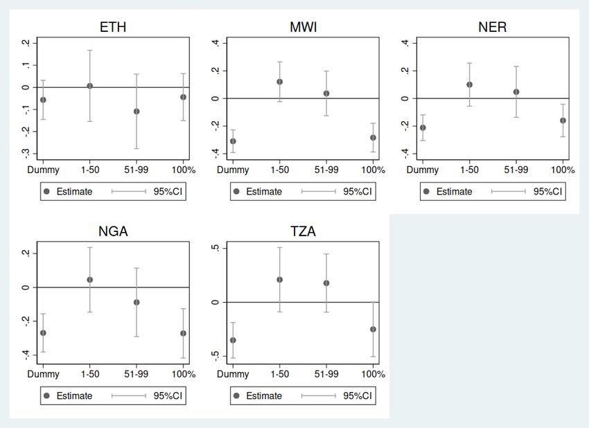
uncovered (Riedel 2007; ISSA 2019). Contributory schemes, however, are still the wider norm. They
    include forms of health insurance or other forms of benefits covering only a small share of the popula-
    tion (mostly public sector and larger companies). Albeit costly and non-holistic, they are considered a
    useful tool to protect individuals, but only a few studies to date look at the evolution of such policies,
    like the impacts of health insurance reforms (Degroote et al. 2019). Measures of this type tend to be
    part of formal contract arrangements, potentially including coverage or providing some security beyond
    the nominal beneficiaries. Where regulations of employment relations have not covered some forms of
    wage employment or provisions of services, they automatically make wage work informal. It is widely
    documented that informality beyond self-employed farm work is highly common in the region among
    wage workers [see, for example, Danquah et al. (2019) or OECD and ILO (2019)].

    Thanks to a mix of global effort to better include social protection programmes into national strategies,
    both political debates and institutional processes have given room for expansion to such policies in SSA
    countries. In addition to a new role that has taken the provision of social protection and particularly so-
    cial security legislation to protect more workers and citizens (ISSA 2019), some researchers argue that
    political pressure over elections may have mattered for the introduction of flagship programmes, whether
    the subject has been endorsed by the incumbent or the contestant party. Taking as an example the most
    budget-constrained country under our analysis, Malawi, Hamer and Seekings (2017) suggest that ex-
    President Banda branded herself with the adoption of multiple social protection initiatives, specifically
    forms of social assistance, and the ineffectiveness of coverage was masked over the period 2012–14
    (prior to the 2015–16 survey into analysis) until delivery during the following mandate.1 Such a trend
    is also observed in Tanzania, where the proposal for the introduction of an old-age pension came within
    one year of a parliamentary and presidential election in October 2015 (Ulriksen 2016). However, the
    expansion of programmes may also come from sectoral- and local-level institutions, as in South Africa
    where agricultural workers were granted coverage under the labour law and the minimum wage provi-
    sion, sparking side effects such as greater compliance in non-wage benefits (Bhorat et al. 2014).

    We thus expect that the coverage of social protection measures in employment relations will be relatively
    low albeit significant, showing differential rates of coverage at individual and household levels according
    to the country and area under analysis.

    3        Data and variables

    3.1       Data

    The data used for this study are the Living Standards Measurement Study - Integrated Surveys on Agri-
    culture (LSMS-ISA) from five countries in SSA, namely Ethiopia, Malawi, Niger, Nigeria, and Tan-
    zania.2 The surveys were chosen for three reasons. First, the comparability of survey questionnaires
    allows construct of the same variables for all countries. Second, all household surveys are nationally
    representative and comprehensively cover both income from and labor input in various livelihood activ-
    ities. This enables us to construct indicators of formality at the household level that go beyond simple
    headcounts of formal workers. Third, in contrast to, for example, Latin American countries, social pro-
    tection policies remain sparse in SSA but are increasingly gaining attention in the policy debate. This

1     The initial ‘branding’ eventually led to a rising significance of such policies in the national agenda that today is represented by
    the second round of the Malawi National Social Support Program II (MNSSP II, 2018–23), which aims to provide three forms
    of assistance: cash and in-kind transfers for household consumption, resilience packages, and measures linked to seasonal and
    humanitarian response to shocks (Government of Malawi 2018).
2    The LSMS-ISA data sets are nationally representative, cross-sectional, and longitudinal surveys conducted by the World
    Bank in collaboration with the national statistical offices.

                                                                     3
study thus aims to assess current reach and implications of existing formal social protection to guide
policy discussions in the region. We focus on urban areas where the scarce opportunities of social pro-
tection through wage employment are most common. However, one main caveat should be highlighted:
there are still limitations across countries in the identification of access to programmes and employment
status or type because of differences in the content of questionnaires across countries. Such differences
will be highlighted when applicable to assess the comparability between countries.
The full breakdown of urban households across each country survey is shown in Table 1.
Table 1: Surveys and urban sample size by country
Country Survey year Sample size (households)
Ethiopia 2015–16 1,682
Malawi 2016–17 2,272
Niger 2014 1,298
Nigeria 2014–15 1,281
Tanzania 2015–16 1,368
Source: authors’ compilation based on LSMS-ISA data.
3.2 Variables
This section presents how the main variables of interest were constructed. Specifically, we aggregate
formality at the household level in two ways: income and full-time equivalents of labour, all expressed
as shares of the household total. Finally, outcome measures of interest are defined.
Formality
In a context where formality of labour is still rare and most activities can be considered informal, we
choose to focus on identifying formal work activities, keeping informality as our base category of analy-
sis. The definition applied is one of activities in an informal sector being broadly characterized by units
engaged in the production of goods or services with the primary objective of generating employment
and income to those engaged (OECD et al. 2002).3 To draw meaningful conclusions for policy with the
individual-level data on employment from the LSMS-ISA data, we focus on formality of wage employ-
ment, and we define formality in terms of the social protection status of workers. While we acknowledge
that the majority of self-employed activities (independent work) in the countries we study is likely to be
informal, we choose to look into wage employment. Formality of small or micro-enterprises is thus not
the focus of this article. The latter may not be easily comparable because of livelihood traits (like the
returns to capital, market exposure, or national availability of private or public schemes for protecting
the self-employed) and the comparative advantage to be in or switch across these forms of employment
(i.e. in terms of time availability to assist seasonal agricultural productions versus those in other forms
of entrepreneurship).
Table 2 presents an overview of the definitions used in each country. A wage work activity is consid-
ered formal with respect to its social protection status if the employer contributes towards a pension
scheme and/or health insurance. Alternative definitions of formality could be via the contract status of
an employee, such as whether they have a signed contract or via employer characteristics (e.g., employer
withholds taxes or has more than five employees). However, these definitions are less comparable across
surveys and insufficiently capture the aspect of protection directly provided to the worker from which
household members could benefit as well. Thus, the social protection definition is preferred and also
3 Note that the informal sector should not be confused with forms of illegal production, domestic production for own final
consumption, or underground activities [see OECD et al. (2002: 39)].
4following the recommendations from the International Conference on Labour Statistics [see ICLS15
(1993); ICLS17 (2003)].
All formality definitions can only apply to those of legal working age, which is 16 in all countries. While
it is likely that younger household members could work, they cannot access formal opportunities, so we
only consider those 16 years and older for our analysis.
Table 2: Formality definition by country
Country Social protection access
Ethiopia If employer is government, state-owned firm, NGO/charity, or political party,
employment comes with health insurance and pension
Malawi If employer provides health insurance and/or pension
Niger If employer provides health insurance and/or pension
Nigeria If employer provides health insurance (and/or pension)*
Tanzania If employer provides health insurance and/or
offers maternity or paternity leave
Note: * only available for cross-sectional analysis. In the panel, we use only access to health insurance.
Source: authors’ compilation based on LSMS-ISA data.
Formality at the household level
We create two measures of informality at the household level: a share of all informal full-time equiv-
alents (FTEs) worked and a share of income from informal sources relative to all income-generating
activities of the household.
FTE shares are computed in the following way. First, all hours worked annually in each activity are
computed for each individual and assigned to be formal or informal. Then, these hours are divided by
the FTE of hours worked in a year. Full-time work is assumed to be 12 months per year, 4.3 weeks per
month, and 40 hours per week, resulting in 2,016 hours per year. All FTEs are replaced to 0 for those
not engaging in any activity, and a maximum of 16 hours of work per day and 52 weeks per year are
imposed. Despite these limits, it is still possible for an individual to have more than two FTEs in total
because of multiple employment activities, so we re-scale these to be a maximum of two per individual
but distributed across various activities in the same proportion as before the capping at two. FTEs are
then summed up at the household level by formal and informal activities, and the share of formal FTEs
over all FTEs of all household members is computed.
To get formal household income shares, we compute the income from each activity that is assigned as
formal or informal and then aggregate these at the household level. The share of income from informal
activities relative to total household income is computed.
Outcome measure
The outcome of interest is a measure of household welfare, measured with poverty status or expendi-
ture.
The household consumption measure was calculated and converted to daily per capita expenditure. For
comparability across countries, expenditures were expressed in purchasing power parity (PPP) in con-
stant US dollars from 2011. This expenditure variable is expressed on a logarithmic scale to reduce the
influence of outliers and express differences in terms of percentages. Poverty is defined with the inter-
national poverty line of US$1.90 consumption per person per day (Ferreira et al. 2016). In the dynamic
analysis for Nigeria, we use the national poverty line for comparability reasons over time.
54 Summary statistics
This section presents summary statistics of the main variables, especially formality measured at the
household level. While most labour market statistics focus on the share of formally employed workers
among the economically active population, the LSMS-ISA data allow assessment of how many house-
holds directly or indirectly benefit from formal employment. Table 3 contrasts these two approaches.
For each country, it shows not only the formal employment share but also the share of households with
a formally employed household member.
Table 3: Share of population covered through formal employment, by country
Country Share of economically active population Share of households with
with formal wage job formal wage income
Ethiopia 0.21 0.26
Malawi 0.14 0.22
Niger 0.11 0.18
Nigeria 0.16 0.19
Tanzania 0.11 0.18
Note: population weights applied to cross-sections for Ethiopia (2015–16), Malawi
(2016–17), Niger (2014), Nigeria (2015–16), and Tanzania (2014–15).
Source: authors’ compilation based on LSMS-ISA data.
While levels of formality vary across countries, the share of households with formal workers is higher
than the simple formal employment share in all countries. If considered at the household level, for-
mality is more prevalent than if only considered among workers. Formally employed workers are most
common in urban Ethiopia followed by urban Nigeria with 21 and 16 per cent, respectively. In the less
economically transformed countries, formal job opportunities remain sparse with just 11 per cent of the
economically active population in urban areas in such employment. Yet, in Niger and Tanzania, 18 per
cent of urban households, respectively, have a member with formal employment.
Figure 1 presents the shares of formal FTEs or income at the household level for each country. Formality
is defined via the provision of social protection through wage employment. All measures are conditional
on at least one household member having a wage income. The light and dark blue bars show the popu-
lation mean of the share of FTEs in a household that are formal, once defined by FTEs (light blue) and
once by income shares (dark blue). The largest formal share can be found in Nigeria for income shares,
while in all other countries, FTE shares tend to be slightly larger. However, FTE and income shares are
always at a comparable level.
6Figure 1: Formality shares of work effort (FTE) and income at household level, population means by country
Note: SP: social protection; FTE: full-time equivalent; population weights applied. Source: authors’ compilation based on
LSMS-ISA data.
5 Depth of informality in a cross-sectional setting
5.1 Estimation strategy
We run a simple regression of the welfare outcome Yi on our informality measure In f and other house-
hold and local characteristics Xi :
Yi = α + β1 Inf1i + β2 Inf2i + β3 Inf3i + β4 Xi + β5 Zl + i (1)
Yi is either the log of per capita expenditure or a simple dummy of whether a household is poor based on
the international poverty line of US$1.90 per day. The variables In fi1 to In fi5 are dummies for different
bins in the distribution of our continuous informality measure. In fi1 is the lowest bin of 0.1 to 50 per
cent of informality, In fi2 is 51 to 99 per cent of informality, and In fi3 captures all observations with
100 per cent, meaning households whose income is earned fully from or all FTEs worked are in the
informal sector. These dummies are all relative to the base category of 0 informal work or income
shares. The logic behind this functional form is to avoid rigidly assuming that there is a linear dose-
response function with respect to a household’s informality mix. We use only four bins because of the
limited sample size. Xi includes the sex and age of the household head, share of household members
with secondary education, household size, dependency ratio, and a dummy whether the household owns
any land. The vector Zl includes dummies for the administrative areas of the highest level to capture
structural differences between regions and a dummy for each tercile of travel distance to the nearest
population centre.
7Figure 2: Share of households within each informality bin, by country
Source: authors’ compilation based on LSMS-ISA data.
The results of these regressions will be contrasted with those of a regression where a simple dummy
for a household head working in the informal sector is used instead of our gradual measure of informal-
ity.
Figure 2 shows the distribution of the informal employment share by country. In Nigeria and Tanzania,
80 per cent or more of all households have fully informal income. In Ethiopia, Malawi, and Niger,
this number is between 70 per cent and 80 per cent. The distribution of informal FTE shares looks
almost identical across countries. The percentage of households with a fully formal income is around
10 per cent in all countries but lower in Nigeria, where relatively more households have a mixed income
portfolio.
Not shown here, we separated the sample into administratively rural and urban defined areas to allow
for structural differences in household income portfolios and access to formal jobs. In all countries, the
share of households with 100 per cent of their income earned from informal activities is more than 80
per cent in rural areas, contrasting urban informality shares between 47 per cent in Malawi and up to 68
per cent in Niger. The cell sizes of observations in the informality bins are accordingly small in the rural
sample. We therefore present our results only for urban areas.
5.2 Results
Regression results are plotted as coefficient graphs for ease of interpretation. The graphs include the
coefficient of the simple household head dummy (’Dummy’) and then plot the three coefficients of each
informality bin compared to the 0 bin (= fully formal).
The full regression results with additional control variables can be found in the Appendix. Results
are as expected: households with female heads are on average poorer, as are households with larger
8household size and those that own land. The latter is highly correlated with agriculture as the main
income source, which in most cases is associated with smallholder farming in the countries of this study.
More household members with secondary education relative to household size is associated with higher
expenditure and lower probability to be poor.
Figures 3 and 4 plot the coefficients of the regressions of poverty status of households on their share
of income earned from informal sources (Figure 3) or the share of FTEs worked in informal activities
(Figure 4). The main finding is that poverty is not in all countries statistically significantly associated
with informality, and it appears that households with both a formal income source and other informal
sources achieve better welfare outcomes than fully informal households and sometimes even better than
fully formal ones. These correlations might indicate that a greater diversification of income sources is
associated with a lower likelihood of being poor. Overall, we observe that the precision of the bins
between fully formal and fully informal is relatively low. This could partially be because of a lack of
power. The first coefficient in each figure is from the dummy of the informal status of the household
head. In Malawi, Niger, and Tanzania, households with an informally employed household head are
significantly more likely to be poor than households with formally employed heads. In the other two
countries, this relationship is insignificant. Only in Tanzania, households are also significantly more
likely to be poor if their income origins are 100 per cent from informal sources. For FTE shares, this
result is also significant for Malawi and Nigeria. In Figures 3 and 4, only Malawi shows a clear and
significant relationship between poverty status and different steps of informality in terms of formal
income shares. Households with some share of formal income are all significantly less likely to be poor
than households with fully formal income or fully informal income. In Ethiopia, this applies to those
households with informal income shares between 0 and 50 per cent and in Niger to households with
more than half of their labor efforts in informal activities. Even though insignificant, similar patterns are
observed in Nigeria for income shares.
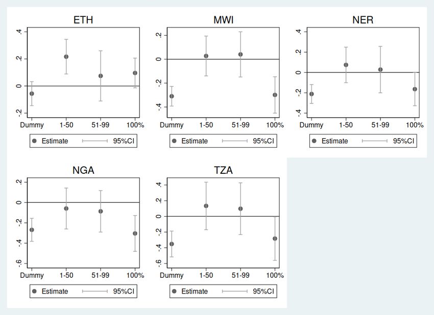
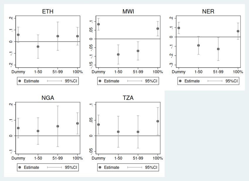
Figures 5 and 6 present the same results for per capita expenditure instead of poverty status. While
poverty status measures whether a household’s expenditure lies below a specific threshold, these results
capture the overall relationship between informality status and expenditure, and they appear more pre-
cise. The main results are that households with an informally working household head have significantly
lower per capita expenditure: around 20 per cent less in Niger, 30 per cent less in Malawi and Nige-
ria, and 40 per cent less in Tanzania. Only in Ethiopia we do not find a significant disadvantage for
informally employed household heads. This is also the case when we consider households with 100 per
cent informal income shares or informal FTE shares. In Malawi, Niger, Nigeria, and Tanzania, the size
of these expenditure gaps are the same as when comparing households with 100 per cent of household
income earned from informal sources to those with fully formal income sources. Looking at the par-
tially formal households, in all countries there are no significant differences between partially formal
and fully formal households. Only in Ethiopia, when using income shares, households less than half of
their income from informal sources are even richer than fully formal households.
The results presented provide interesting insights in three aspects. First, the informality status of a
household head is strongly associated with our measure of fully informal households in terms of in-
come shares or FTE shares. However, they do not yield always the same results, and most importantly,
the simple household head measure obscures important nuances of household income generation and
welfare. These are revealed in the second finding. That is, households with a mix of income sources
or activities show better welfare outcomes than fully informal households and, in some countries, even
better outcomes than fully formal households. It appears that households with a formally employed
member fare even better if the household earns other income or spends time in other activities that are in
the informal sector, controlling for household size and dependency ratio. In some countries, an income
or activity share in formal activities of less than half can already make the household better off than fully
informal income generation. The results are starker and more precise when we consider expenditure
compared to poverty status. This is not surprising given the small cell sizes and that the expenditure re-
9Figure 3: Coefficients of informality measures from regression of probability to be poor. Share of income earned from informal
sources. Base category is fully formal income.
Note: the graphs plot coefficients and confidence intervals (CI) from two different regressions for each country. The first
coefficient is that of the dummy indicating an informal household head from one regression. The other three coefficients are
those of the informality bins from the regression as specified in 1. The base category is households with no informal income
source.
Source: authors’ compilation based on LSMS-ISA data.
10Figure 4: Coefficients of informality measures from regression of probability to be poor. Share of FTEs worked in informal
activities. Base category is fully formal activities.
Note: the graphs plot coefficients and confidence intervals (CI) from two different regressions for each country. The first
coefficient is that of the dummy indicating an informal household head from one regression. The other three coefficients are
those of the informality bins from the regression as specified in 1. The base category are households with no informal income
source.
Source: authors’ compilation based on LSMS-ISA data.
11Figure 5: Coefficients of informality measures from regression of per capita expenditure. Share of income earned from informal
sources. Base category is fully formal income.
Note: the graphs plot coefficients and confidence intervals (CI) from two different regressions for each country. The first
coefficient is that of the dummy indicating an informal household head from one regression. The other three coefficients are
those of the informality bins from the regression as specified in 1. The base category are households with no informal income
source.
Source: authors’ compilation based on LSMS-ISA data.
12Figure 6: Coefficients of informality measures from regression of per capita expenditure. Share of FTEs worked in informal
activities. Base category is fully formal activities.
Note: the graphs plot coefficients and confidence intervals (CI) from two different regressions for each country. The first
coefficient is that of the dummy indicating an informal household head from one regression. The other three coefficients are
those of the informality bins from the regression as specified in 1. The base category are households with no informal income
source.
Source: authors’ compilation based on LSMS-ISA data.
13gression exploits more variation than the linear probability model of poverty. Lastly, comparing results
using income shares with those using FTE shares, we find comparable patterns. This encourages the
applicability of our measure in contexts when only income or only work hour data are available.
6 Depth of informality in a dynamic setting
So far, we have compared households at a specific point in time for each country and established some
empirical patterns in the relationship between household welfare and depth of informality. The next
question to ask about this relationship is whether changes in the depth of informality within a household
are associated with improvements in welfare. In this section, we thus take a dynamic perspective that
also accounts for several econometric concerns arising in the cross-sectional analysis.
The limits of estimating (1) in a cross-section lie in the presence of unobserved characteristics that,
on one hand, may determine simultaneously a household’s income portfolio and its welfare outcomes.
On the other hand, such traits could predict a household’s selection into formal or informal income-
generating activities. These issues can be addressed with longitudinal data in which we observe house-
holds in several time periods. In general, there are examples in the literature that capture the information
contained in panel data to investigate transitions between the informal and formal sector (Bosch and
Maloney 2010; Danquah et al. 2019). However, to the best of our knowledge, none of this literature has
considered informality transitions more widely as a household decision.
To that aim, we use three waves of the Nigerian LSMS-ISA panel data, namely waves 1–3 corresponding
to 2010, 2012, and 2015–16,4 as well as two waves of the Tanzanian panel, from 2010 and 2012. We
use only FTE shares to measure the depth of informality again because of varying questionnaire designs
that did not allow us to capture income shares consistently. However, based on the cross-sectional
results, we are confident that the dynamic FTE results would be very similar if we used income shares
instead.
6.1 Estimating transitions
We define three categories of depth of informality: fully informal (I), mixed portfolio (M), and fully
formal (F). Then we assess transitions over time between these states. Our dynamic analysis proceeds in
three steps. First, we document the differences in welfare by each type of transition that a household can
make. Then we focus these transitions on the directions of interest that are in and out of full informality.
Lastly, we apply the most robust definition of control groups and transition directions to control also for
selection bias.
For the first part, households may switch status from one of three types into any permutation. This
yields six possible transitions that a household may do over two periods and three instances of staying
put. We compute statistics of the means before and after transition by type of switcher. Tables 4 and
5 present the results of a simple longitudinal analysis on these data. We compare transitions across a
one-period ‘hop’, so we are only ever considering the short-run effects of moving from one status to
another. In the data from Tanzania, this corresponds to two years and in Nigeria to two and three years.
This approach is adopted to mitigate any potential issues in time-series estimation such as inconsistent
standard errors caused by serial correlation, as raised by Bertrand et al. (2004). Both tables record the
mean outcome for the relevant group’s welfare indicator before and after their transition. Columns (3)
in the tables present the raw gap between the relevant group and the never-changers group relative to
staying in one’s origin for both periods. For example, this would imply that for those going from having
4 The latest wave of the Nigerian panel from 2018 was not consistent in the variable definitions, so we rely on the older waves.
14a fully informal household portfolio to a mixed portfolio are compared with those households who across
two periods would always remain informal. Columns (4) present the conditional gap where we control
for land ownership, female headship, share of secondary school leavers, and year fixed effects. These
estimates treat the data as a cross-section. Finally, columns (5) provide the two-way fixed effects results.
While there is variation in the estimates in columns (5), we observe a general pattern. The two-way
fixed effects estimates are generally smaller than the cross-sectional estimates. This suggests that, to
the extent that anything is uncovered in the cross-section, these estimates may not ultimately hold up
in longitudinal analysis as estimated effects rely on variation from groups that may not be appropriate
control groups. For the majority of comparisons, the two-way fixed effects estimates are at least half the
size of the cross-sectional estimate.5
The second pane of Tables 4 and 5 provide estimates of composite groups who transition in the same ‘di-
rection’ as well as composite control groups who may serve as suitable counterfactuals for these groups.
We estimate pre- and post-transition means, conditional and unconditional gaps, and a two-way fixed
effects regression for those joining informality (i.e. those moving into a fully informal portfolio—MI &
FI movers). These are compared to those households who remained always in the formal sector, either
fully formal or mixed. Notably for this comparison, those transitioning between these statuses are no
worse off after transitioning compared with the stayers when comparing both of our welfare measures.
Similarly, we contrast those leaving informality, both from mixed portfolio households and fully in-
formal households, with those who are always informal and always mixed. For this comparison, it is
worth noting that whilst the cross-section results implied decreases in the conditional and unconditional
probability of being poor, no such change is detected across time, whereas we do detect an increase in
household expenditure as a consequence of the transition. As in the cross-sectional results, expenditure
estimates provide more variation, as those remaining always below or above the poverty threshold might
still experience changes in their expenditure levels.
We further consider the effects of diversifying a household’s portfolio compared to leaving mixed port-
folios. Yet, it should not be surprising that for both of these we do not observe any differences in the
two-way fixed effects approach.
5 It is worth noting that as we report the unconditional means for all transition groups, it should be straightforward for the
reader to estimate a naive differences-in-differences for any comparison group, if preferred over the ones we have selected.
15Table 4: Poverty, log total expenditure, by status and transition, Nigeria 2010–15
P(Poor=1) ln(TotExp)
(1) (2) (3) (4) (5) (1) (2) (3) (4) (5)
Portfolio v control Before After Raw ∆ Cond ∆ DiD Before After Raw ∆ Cond ∆ DiD
II v FF 0.179*** 0.177*** 0.140*** 0.136*** 0.017 4.771*** 5.322*** -0.512*** -0.501*** -0.021
(0.009) (0.008) (0.018) (0.019) (0.035) (0.025) (0.026) (0.137) (0.072) (0.079)
N 2,018 2,018 4,168 4,168 4,168 2,018 2,018 4,168 4,168 4,168
FI v FF 0.098** 0.073* 0.047 0.035 0.005 5.292*** 5.826*** 0.000 0.056 -0.043
(0.047) (0.041) (0.045) (0.042) (0.050) (0.209) (0.246) (0.257) (0.148) (0.131)
N 41 41 214 214 214 41 41 214 214 214
IF v II 0.104*** 0.125*** 0.077** 0.078** 0.039 4.757*** 5.605*** -0.378** -0.203** 0.212**
(0.031) (0.034) (0.032) (0.030) (0.045) (0.132) (0.147) (0.187) (0.097) (0.105)
N 96 96 324 324 324 96 96 324 324 324
FF v II 0.045* 0.030 -0.140*** -0.136*** -0.017 5.279*** 5.839*** 0.512*** 0.501*** 0.021
(0.026) (0.021) (0.018) (0.019) (0.035) (0.139) (0.150) (0.137) (0.072) (0.079)
N 66 66 4,168 4,168 4,168 66 66 4,168 4,168 4,168
MI v MM 0.141*** 0.156*** 0.058 0.067* 0.026 4.918*** 5.768*** 0.258 0.104 0.106
(0.044) (0.046) (0.045) (0.040) (0.064) (0.132) (0.148) (0.159) (0.104) (0.121)
N 64 64 282 282 282 64 64 282 282 282
IM v II 0.121*** 0.100*** -0.067*** -0.091*** -0.028 4.701*** 5.181*** -0.105 0.269*** 0.051
(0.028) (0.025) (0.023) (0.021) (0.033) (0.099) (0.092) (0.089) (0.058) (0.075)
N 140 140 4,316 4,316 4,316 140 140 4,316 4,316 4,316
MM v II 0.091*** 0.091*** -0.087*** -0.107*** -0.001 4.822*** 5.348*** 0.038 0.212*** -0.030
(0.033) (0.033) (0.029) (0.028) (0.034) (0.105) (0.111) (0.102) (0.065) (0.076)
N 77 77 4,190 4,190 4,190 77 77 4,190 4,190 4,190
MF v MM 0.040 0.000*** -0.071** -0.070* -0.044 4.945*** 5.720*** 0.248 0.176* -0.027
(0.040) (0.035) (0.037) (0.053) (0.230) (0.183) (0.212) (0.104) (0.177)
N 25 25 204 204 204 25 25 204 204 204
FM v FF 0.095 0.095 0.057 0.049 0.028 5.345*** 5.471*** -0.151 -0.141 -0.292
(0.066) (0.066) (0.067) (0.064) (0.054) (0.201) (0.175) (0.214) (0.132) (0.206)
N 21 21 174 174 174 21 21 174 174 174
Note: table continued on next page.
16Table 4—continued from previous page
P(Poor=1) ln(TotExp)
(1) (2) (3) (4) (5) (1) (2) (3) (4) (5)
Portfolio v control Before After Raw ∆ Cond ∆ DiD Before After Raw ∆ Cond ∆ DiD
Joiners M (FM&IM v FF&MM) 0.118*** 0.099*** 0.042 0.034 -0.022 4.785*** 5.219*** -0.302*** -0.089 0.007
(0.026) (0.024) (0.027) (0.026) (0.036) (0.091) (0.083) (0.115) (0.070) (0.090)
N 161 161 608 608 608 161 161 608 608 608
Leavers M (MF&MI v FF&MM) 0.112*** 0.112*** 0.046 0.040 0.014 4.925*** 5.755*** 0.036 -0.005 0.021
(0.034) (0.034) (0.031) (0.029) (0.048) (0.114) (0.118) (0.134) (0.080) (0.100)
N 89 89 464 464 464 89 89 464 464 464
Note: this table gives means and estimates of the effect of transitioning as household to/from informality. Groups are defined by their state across the transition gap, so for someone who is always
formal (FF), always informal (II), always mixed (MM), and permutations thereof. Columns (1)&(2) provide the raw means for each portfolio group, in the respective time. Columns (3)&(4) provide the
gap relative to their respective ‘control groups’ estimated as a simple intercept shift using ordinary least squares (OLS). For columns (4)&(5) the estimates are conditional on household size, share
of secondary school leavers, and ‘real-time’ fixed effects. Columns (5) are estimated using a household fixed effects model. The data are stacked on a dimensionless ‘transition time’ that is the gap
in time between period 0 & 1, but naturally this duplicates observations in ‘real time’ in wave 2 in 2012. Errors are clustered at the household level.
Source: authors’ compilation based on LSMS-ISA data.
17Table 5: Poverty, log total expenditure, by status and transition, Tanzania 2012–14
P(Poor=1)
(1) (2) (3) (4) (5) (1) (2) (3) (4) (5)
LHS Before After Raw ∆ Cond ∆ DiD Before After Raw ∆ Cond ∆ DiD
II v FF 0.118*** 0.074** -0.029 -0.075 0.143 1.193*** 1.471*** 0.041 0.271** -0.189
(0.039) (0.032) (0.113) (0.107) (0.225) (0.073) (0.079) (0.200) (0.123) (0.386)
N 68 68 144 144 144 68 68 144 144 144
FI v FF 0.125 0.000*** -0.063 -0.065 0.014 1.476*** 1.695*** 0.294 0.321 -0.004
(0.085) (0.120) (0.128) (0.217) (0.145) (0.122) (0.224) (0.195) (0.369)
N 16 16 40 40 40 16 16 40 40 40
IF v II 0.286** 0.000*** 0.018 -0.016 -0.026 1.232*** 2.019*** 0.334 0.489*** -0.031
(0.101) (0.123) (0.117) (0.228) (0.199) (0.106) (0.233) (0.173) (0.457)
N 21 21 50 50 50 21 21 50 50 50
FF v II 0.250 0.000*** 0.029 0.075 -0.143 0.860* 1.723** -0.041 -0.271** 0.189
(0.250) (0.113) (0.107) (0.225) (0.379) (0.382) (0.200) (0.123) (0.386)
N 4 4 144 144 144 4 4 144 144 144
MI v MM 0.080 0.000*** 0.040 0.041 -0.077 1.499*** 1.546*** -0.275** -0.285** -0.335*
(0.055) (0.028) (0.029) (0.055) (0.131) (0.117) (0.137) (0.130) (0.194)
N 25 25 84 84 84 25 25 84 84 84
IM v II 0.273** 0.000*** 0.041 0.033 -0.294*** 1.249*** 1.698*** 0.142 0.178* 0.442***
(0.097) (0.055) (0.050) (0.109) (0.163) (0.089) (0.113) (0.093) (0.156)
N 22 22 180 180 180 22 22 180 180 180
MM v II 0.000*** 0.000*** -0.096*** -0.094*** 0.055 1.625*** 1.969*** 0.465*** 0.485*** 0.009
(0.026) (0.031) (0.053) (0.145) (0.095) (0.112) (0.116) (0.180)
N 17 17 170 170 170 17 17 170 170 170
MF v MM 0.000*** 0.000*** 0.000*** 0.000*** 0.000*** 1.639*** 2.078*** 0.061 0.005 -0.161
(0.171) (0.233) (0.162) (0.124) (0.204)
N 7 7 48 48 48 7 7 48 48 48
FM v FF 0.077 0.000*** -0.087 -0.127 0.028 1.741*** 1.959*** 0.559** 0.806*** 0.056
(0.077) (0.120) (0.133) (0.220) (0.183) (0.153) (0.229) (0.186) (0.368)
N 13 13 34 34 34 13 13 34 34 34
Note: table continued on next page.
18Table 5—continued from previous page
P(Poor=1)
(1) (2) (3) (4) (5) (1) (2) (3) (4) (5)
LHS Before After Raw ∆ Cond ∆ DiD Before After Raw ∆ Cond ∆ DiD
Joiners I (MI&FI v FF&MM) 0.098** 0.000*** 0.025 0.031 -0.067 1.490*** 1.604*** -0.154 -0.179 -0.228
(0.047) (0.033) (0.037) (0.069) (0.097) (0.085) (0.120) (0.119) (0.185)
N 41 41 124 124 124 41 41 124 124 124
Leavers I (MF&IF v II&MM) 0.214** 0.000*** 0.031 0.046 -0.152* 1.334*** 2.034*** 0.259** 0.161 0.203
(0.079) (0.044) (0.045) (0.089) (0.157) (0.096) (0.113) (0.102) (0.176)
N 28 28 226 226 226 28 28 226 226 226
Joiners M (FM&IM v FF&MM) 0.200*** 0.000*** 0.076* 0.081* -0.237** 1.432*** 1.795*** -0.087 -0.055 0.126
(0.069) (0.042) (0.045) (0.092) (0.128) (0.081) (0.126) (0.132) (0.194)
N 35 35 112 112 112 35 35 112 112 112
Leavers M (MF&MI v FF&MM) 0.062 0.000*** 0.007 0.008 -0.014 1.529*** 1.663*** -0.105 -0.095 -0.344*
(0.043) (0.032) (0.034) (0.063) (0.108) (0.110) (0.128) (0.122) (0.189)
N 32 32 106 106 106 32 32 106 106 106
Note: this table gives means and estimates of the effect of transitioning as a household to/from informality. Groups are defined by their respective state across the transition gap, for someone who is
always formal (FF), always informal (II), always mixed (MM), and permutations thereof. Columns (1)&(2) provide the raw means for each portfolio group, in the respective time. Columns (3)&(4)
provide the gap relative to their respective ‘control groups’ estimated as a simple intercept shift using OLS. For Columns (4)&(5), the estimates are conditional on household size and share of
secondary school leavers. Columns (5) apply a household fixed effects model. Errors are clustered at the household level. ***, **, and * indicate significance at the 1, 5, and 10 per cent critical level,
respectively.
Source: authors’ compilation based on LSMS-ISA data.
19In a final step, we aim to more directly relate the dynamic switches to the findings in the cross-country
cross-sectional analysis where we gained two insights. First, household head informality is as bad
as a fully informal household income portfolio with regards to household welfare and vice versa for
formality. Secondly, households with a mixed income portfolio are not worse off than fully formal
households, and they are better off than fully informal households. To test whether our findings from
the cross-sectional analysis also hold in the longitudinal context, we derive six hypotheses:
H1 Becoming a household with an informal head is as bad as becoming a fully informal household.
H2 Becoming a household with a formal head is as good as becoming a fully formal household.
H3 Households that diversify their income portfolio to a mixed one from previously being fully formal
are not worse off than before.
H4 Households that diversify their income portfolio to a mixed one from previously being fully infor-
mal are better off than before.
H5 Diversified households who collapse their portfolio to formality will only do so if they are as well
off as before.
H6 Diversified households who collapse their portfolio to informality will only do so if they are as
well off as before.
Following advances in the difference-in-difference literature, we estimate these dynamics in difference
in a 2x2 two-way fixed effects estimation setup as proposed by Goodman-Bacon (2018). We deal with
the differential treatment timings by focusing solely on one-period ‘hops’ and ‘stacking’ the data on a
timeless ‘transition time’. We then estimate 2 as follows:
Yi,t = αi + β Postt + δ Switcher × Posti,t + X 0 γi,t (2)
where Yi,t , the welfare outcome of household i in time t, is predicted by a time invariant indicator whether
a household changes its income portfolio, Switcher, between t and t-1 and the dummy, Post, indicating
the second time period in which a household is observed and the interaction of both indicators. δ is
the coefficient of interest showing the effect of the household’s change in status on its welfare. We also
control for a vector of household time-varying characteristics, X (viz. household size and share with
secondary schooling). Further controls used in the cross-sectional case, such as land ownership and
female headship, were considered but ultimately deemed to be potential sources of collider bias in the
dynamic setup, as the parameters would be identified only for those switching status. Those ‘switchers’
amongst the land and household head composition would therefore likely correlate with the switch in
informal household status, expected to bias the estimates of the effect of interest.
With this setup, we automatically eliminate any time-invariant unobserved household characteristics that
determine a household’s welfare outcomes. However, the issue of selection remains. Imagine we com-
pare households that are fully informal in t − 1, and now we define those as switchers who change their
income portfolio to mixed in t and continue to compare them to those who remain fully informal. It is
likely that those who remain fully informal are fundamentally different from those switchers, for exam-
ple because of higher risk aversion. We would thus not compare like with like. Therefore, we design our
control group more carefully by exploiting different treatment timings. With three time periods, we can
identify up to two switches for each household, and we can identify those households who never switch.
These do not serve as good control for our switchers. Instead, we use those households who switch be-
tween the first two periods (‘early switchers’). They serve as comparison to those households who move
in the same direction but only between the last two periods (‘late switchers’). We believe this is the
most robust choice for exploring employment transition dynamics in an endogenous decision-making
process.
20More specifically, we look at the following switchers to test the hypotheses above:
H1 Fully formal household switched to fully informal
H2 Fully informal household switched to fully formal
H3 Fully formal household switched to mixed portfolio
H4 Fully informal household switched to mixed portfolio
H5 Mixed portfolio household switched to fully formal
H6 Mixed portfolio household switched to fully informal
The control groups are defined accordingly as those who switched early, while the treated are those who
switched later (groups switching from period T1 to T2 are used as comparison for those moving from
T2 to T3). While all our data sets are one round of a panel survey, because of inconsistencies in data
collection over time for variables most relevant to our study, we can only use three waves of the Nigeria
survey. Using a two-wave panel as available in Tanzania would not overcome the issue of selection,
while it can be resolved with the above described strategy for Nigeria.
To illustrate how comparable early and late switcher households are in our sample, we present pre-
switching balance statistics in Table 6. Each broad column shows the balance tests of one sample related
to one specific hypothesis test. The table demonstrates that we compare statistically similar households
based on their observable characteristics that we use as controls. We note, however, that especially when
investigating switchers from formal to informal or mixed income portfolios, the sample is very small,
especially for the control groups of early switchers. To confirm whether estimated effects are true or a
result of low power, we will conduct randomization inference of the point estimates we obtain from the
two-way fixed effects as a robustness check.
Table 7 reports the results of estimation (2); each cell represents the estimate for the δ parameter. The
purpose of this estimation strategy is to ensure that any unobserved heterogeneity that may bias the
estimates is cancelled out, as we focus our estimates on those who transition compared to those who
transition in the same direction, in the following wave. This gives the average treatment effect on the
treated, conditioning out the potential endogenous unobservables that influence the decision for a house-
hold to change its formality status. It is worthwhile remarking that when this is done, no comparison is
found to be significant. That is, no transition is found to differently affect a household’s welfare. The
only transition subgroup for which we can detect any difference is those who move from full formality
into a mixed portfolio. There we observe no change on the probability of being poor, but there is a
decline in total expenditure of 32.6 per cent. This is consistent with the view that households may be
subject to covariate shocks that may make their welfare decrease but by hedging household trade-off
consumption levels to adjust to this change. However, households are not pushed into poverty by this
move.
It is a stark finding that regardless of the other direction of transitions, there are no effects detected on
household welfare measures. It is, however, worth bearing in mind that some of the cells of switchers
are very small, which would put inference drawn from these estimates under suspicion, calling for a
thorough inspection in this sense in the next section.
21You can also read