XCO2 estimates from the OCO-2 measurements using a neural network approach - AMT
←
→
Page content transcription
If your browser does not render page correctly, please read the page content below
Atmos. Meas. Tech., 14, 117–132, 2021
https://doi.org/10.5194/amt-14-117-2021
© Author(s) 2021. This work is distributed under
the Creative Commons Attribution 4.0 License.

XCO2 estimates from the OCO-2 measurements using
a neural network approach
Leslie David, François-Marie Bréon, and Frédéric Chevallier
Laboratoire des Sciences du Climat et de l’Environnement/IPSL, CEA-CNRS-UVSQ,
Université Paris-Saclay, 91198 Gif-sur-Yvette, France

Correspondence: François-Marie Bréon (fmbreon@cea.fr)

Received: 5 May 2020 – Discussion started: 2 June 2020
Revised: 14 November 2020 – Accepted: 16 November 2020 – Published: 7 January 2021

Abstract. The Orbiting Carbon Observatory (OCO-2) instru-          1   Introduction
ment measures high-resolution spectra of the sun’s radiance
reflected at the earth’s surface or scattered in the atmosphere.   During the past decades, natural fluxes have absorbed about
These spectra are used to estimate the column-averaged dry         half of the anthropogenic emissions of CO2 (Knorr, 2009),
air mole fraction of CO2 (XCO2 ) and the surface pressure.         but there is large uncertainty about the spatial distribution of
The official retrieval algorithm (NASA’s Atmospheric CO2           this sink over time and therefore on the processes that control
Observations from Space retrievals, ACOS) is a full-physics        it. A growing network of high-precision atmospheric CO2
algorithm and has been extensively evaluated. Here we pro-         measurements has been used together with meteorological
pose an alternative approach based on an artificial neural net-    information to constrain the sources and sinks of CO2 using
work (NN) technique. For training and evaluation, we use           a technique known as atmospheric inversion (e.g., Peylin et
as reference estimates (i) the surface pressures from a nu-        al., 2013), but the lack of data in large regions of the globe,
merical weather model and (ii) the XCO2 derived from an            such as the tropics, does not allow the monitoring of these
atmospheric transport simulation constrained by surface air-       fluxes with enough space–time resolution. Early attempts to
sample measurements of CO2 . The NN is trained here us-            complement this network with satellite retrievals from sen-
ing real measurements acquired in nadir mode on cloud-free         sors that were not specifically designed for this purpose were
scenes during even-numbered months and is then evaluated           not successful (Chevallier et al., 2005), but a series of ded-
against similar observations during odd-numbered months.           icated instruments were put into orbit when the Greenhouse
The evaluation indicates that the NN retrieves the surface         Gases Observing Satellite (GOSAT, Yokota et al., 2009) and
pressure with a root-mean-square error better than 3 hPa and       the second Orbiting Carbon Observatory (OCO-2 Eldering
XCO2 with a 1σ precision of 0.8 ppm. The statistics indi-          et al., 2017) were launched in 2009 and 2014, respectively.
cate that the NN trained with a representative set of data al-     These were still operational at the time of writing. This new
lows excellent accuracy that is slightly better than that of the   and evolving constellation is directly supported by Japanese,
full-physics algorithm. An evaluation against reference spec-      US, Chinese, and European space agencies (CEOS Atmo-
trophotometer XCO2 retrievals indicates similar accuracy for       spheric Composition Virtual Constellation Greenhouse Gas
the NN and ACOS estimates, with a skill that varies among          Team, 2018). All missions have adopted the same CO2 ob-
the various stations. The NN–model differences show spa-           servation principle that consists of measuring the solar irradi-
tiotemporal structures that indicate a potential for improving     ance reflected at the earth’s surface in selected spectral bands.
our knowledge of CO2 fluxes. We finally discuss the pros and       Along the double atmospheric path (down-going and up-
cons of using this NN approach for the processing of the data      going), the sunlight is absorbed by atmospheric molecules
from OCO-2 or other space missions.                                at specific wavelengths. The resulting absorption lines on the
                                                                   measured spectra make it possible to estimate the amount of
                                                                   gas between the surface and the top of the atmosphere. CO2
                                                                   shows many such absorption lines around 1.61 and 2.06 µm

Published by Copernicus Publications on behalf of the European Geosciences Union.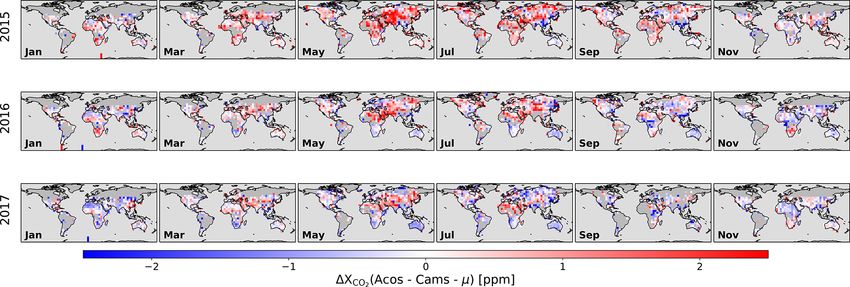
118                                                           L. David et al.: A neural network approach for XCO2 retrieval

that are used to estimate the CO2 column. Similarly, the oxy-      use real OCO-2 observations together with collocated esti-
gen lines around 0.76 µm are used to estimate the surface          mates of the surface pressure and XCO2 . The retrievals from
pressure and can also be used to infer the sunlight atmo-          the NN approach are evaluated against model estimates of
spheric path, leading to the column-averaged dry air mole          surface pressure and XCO2 , as well as observations from the
fraction of CO2 , referred to as XCO2 (O’Brien and Rayner,         Total Carbon Column Observing Network (TCCON, Wunch
2002; Crisp et al., 2004).                                         et al., 2011a). In the following, Sect. 2 presents the approach
   One main difficulty in the retrieval of XCO2 from the mea-      while Sect. 3 describes the results. Section 4 discusses the
sured spectra results from the presence of atmospheric par-        results and the way forward.
ticles that scatter light and change its atmospheric path. Ac-
counting for aerosols, in particular, is challenging because
aerosols are highly variable in amount and in vertical dis-        2   Data and method
tribution. Another major difficulty results from modeling er-
rors. The radiative transfer models that are used for the re-      Our NN estimates XCO2 and the surface pressure from nadir
trieval leave significant residuals between the measured and       spectra measured by the OCO-2 satellite over land. OCO-2
modeled spectra, even after the XCO2 and aerosol amount            has eight cross-track footprints (e.g., Eldering et al., 2015),
have been inverted for a best fit (Crisp et al., 2012; O’Dell et   but we only use footprint #4 in the following for simplicity.
al., 2018). As a consequence of the various uncertainties in       If successful, the same approach can be applied to all foot-
the retrieval process, raw XCO2 retrievals show significant        prints. The focus on nadir measurements here is motivated
biases against reference ground-based retrievals (Wunch et         by the complication introduced by the Doppler effect in glint
al., 2011b, 2017). These biases, together with the comparison      mode, which is the other pointing mode for OCO-2 routine
against modeling results, led to the development of empirical      science operations: the absorption lines affect pixel elements
corrections to the retrieved XCO2 . In the case of the OCO-2       that vary among the spectra. These variations of the position
V8r retrievals generated by NASA’s Atmospheric CO2 Ob-             of the absorption line may cause additional difficulty to the
servations from Space (ACOS), these corrections amount to          NN training. The solar lines in the nadir spectra are also af-
roughly half that of the “signal”, i.e., of the difference be-     fected by Doppler shifts due to the motion of the earth and
tween the prior and the retrieved XCO2 (O’Dell et al., 2018).      satellite relative to the sun, but this concerns a limited set of
   The limitations in the full-physics retrieval method, de-       spectral elements that are affected by the solar (Fraunhofer)
spite considerable effort and progress (e.g., O’Dell et al.,       lines. The development of a glint-mode NN is therefore left
2018; Reuter et al., 2017; and Wu et al., 2018 in the case of      for a future study.
OCO-2), encourage developing alternative approaches. Here,            We use spectral samples in the three bands of the instru-
we want to re-evaluate the potential of an artificial neural       ment (around 0.76, 1.61 and 2.06 µm). They have footprints
network technique (NN) to estimate XCO2 from the mea-              of ∼ 3 km2 on the ground. In principle, each band is de-
sured spectra. A NN-based technique was already used by            scribed by 1016 pixel elements, but some are marked as bad
Chédin et al. (2003) for a fast retrieval of midtropospheric       either because some of the corresponding detectors have died
mean CO2 concentrations from some meteorological satel-            or because of known temporary or permanent issues. We
lite radiometers. These authors trained their NNs on a large       systematically remove 15 pixel elements that are flagged in
ensemble of radiance simulations made using a reference ra-        about 80 % of the spectra and 478 pixels in the band edges.
diation model and assuming diverse atmospheric and surface         Conversely, we do not remove the spectra that are affected by
conditions. NN-based approaches are also commonly used             the deep solar lines and we let the NN handle these specific
for the retrieval of other species from various high-spectral-     features. Because the information in the spectrum is mostly
resolution satellite radiance measurements because of their        in the relative depth of the absorption lines, and not in their
computational efficiency (e.g., Hadji-Lazaro et al., 1999).        overall amplitude, we normalize each spectrum by a radiance
   A NN approach requires a large and representative train-        that is representative of the offline values (i.e., the mean of
ing dataset. A standard method for problems similar to that        the 90 %–95 % range for each spectrum). This essentially re-
discussed here is to use a radiative transfer model and to         moves the impact of the variations in the surface albedo and
generate a large ensemble of pseudo-observations based on          in the sun irradiance linked to the solar zenith angle. Other
assumed atmospheric and surface parameters. However, as            input choices may be attempted in the future.
mentioned above, the radiative transfer models have deficien-         As input to the NN, we add the observation geometry
cies that are rather small, but nevertheless significant with      (sun zenith angle and relative azimuth). The sun zenith an-
respect to the high-precision objective of the CO2 measure-        gle drives the atmospheric pathlength and is then required
ments. In addition, there may be some wrong assumptions            for the interpretation of the absorption line depth in terms of
and unknown instrumental defects that are not accounted for        atmospheric optical depth. The azimuth was not included in
in the forward modeling. We thus prefer to avoid using such        our first attempts, but when later included it led to a signifi-
radiative transfer models and rather base the training on a        cant improvement in the results. Although the NN technique
fully empirical approach (see, e.g., Aires et al., 2005). We       does not allow for a clear physical interpretation, we assume

Atmos. Meas. Tech., 14, 117–132, 2021                                                 https://doi.org/10.5194/amt-14-117-2021
L. David et al.: A neural network approach for XCO2 retrieval                                                                  119

that the information brought by the relative azimuth is linked     use less restrictive criteria and accept observations with out-
to the polarization of the molecular scattering contribution to    come_flag of either 1 or 2, and cloud_flag of 2 or 3. These
the measurements that varies with the azimuth.                     choices are justified below. The spatial distribution of the ob-
    The NN exploits these 2557 input variables to compute          servations that are used for the training is shown in Fig. A2
two variables only: XCO2 and the surface pressure. It is           of the Appendix. The training dataset covers most regions of
structured as a multilayer perceptron (Rumelhart et al., 1988)     the globe with the exception of South America. The under-
with one hidden layer of 500 neurons that use a sigmoid acti-      representation of this subcontinent stems from both the high
vation function. The number of hidden layers is somewhat ar-       cloudiness and impact of cosmic rays that leads to missing
bitrary and based on a limited sample of trials. Lower quality     pixel elements (see below).
estimates were obtained with 50 neurons whereas the train-            For the reference surface pressure (training and evalua-
ing time increased markedly for 1000 neurons and more. The         tion), an obvious choice is the use of numerical weather anal-
weights of the input variables to the hidden neurons and the       yses corrected for the sounding altitude. Indeed, the typical
weights of the hidden variables to the output variables are        accuracy for surface pressure data is on the order of 1 hPa
adjusted iteratively with the standard Keras library (Keras        (Salstein et al., 2008). For convenience, we use the surface
Team, 2015). Figure A1 in the Appendix illustrates the con-        pressure that is provided together with the OCO-2 data and
vergence process. The NN cost function (a.k.a. loss) becomes       is derived from the Goddard Earth Observing System, Ver-
fairly constant for a test dataset after about 100 iterations,     sion 5, Forward Processing for Instrument Teams (GEOS5-
whereas it continues to decrease for the training dataset, in-     FP-IT) created at the Goddard Space Flight Center Global
dicating an overfitting of the data. The iteration is stopped      Modeling and Assimilation Office (Suarez et al., 2008; and
when there is no decrease of the test loss for 50 iterations.      Lucchesi et al., 2013). There is no such obvious choice for
There is a factor of 3 to 4 between the loss of the training       XCO2 as there is no global-scale highly accurate dataset of
dataset and that of the test, which confirms the overfitting of    XCO2 and we thus rely here on best estimates from a model-
the former.                                                        ing approach. We use the CO2 atmospheric inversion of the
    Note that the NN estimate does not use any a priori in-        Copernicus Atmosphere Monitoring Service (CAMS, http:
formation on surface pressure or the CO2 profile after the         //atmosphere.copernicus.eu, last access: 28 January 2020,
training is done. Also, no explicit information is provided on     Chevallier et al., 2010; version 18r2). This product was re-
the altitude, location, or time period of the observation. The     leased in July 2019 and contributed, e.g., to the Global Car-
NN estimates are therefore only driven by the OCO-2 spec-          bon Budget 2019 of Friedlingstein et al. (2019). It results
trum measurements, together with the observation geometry          from the assimilation of CO2 surface air-sample measure-
(sun zenith and relative azimuth). The observation geometry        ments in a global atmospheric transport model run at spatial
varies with the latitude and the season so that the NN may         resolution 1.90◦ in latitude and 3.75◦ in longitude over the
infer some location information from this input. Conversely,       period from 1979–2018 and using the adjoint of this trans-
it is the same from one year to the next and, at a given date,     port model. Neither satellite retrievals nor TCCON observa-
for all longitudes. Thus, there is no information on the lon-      tions were used for this modeling. For each OCO-2 obser-
gitude or the year of observation in the geometry parameters       vation, XCO2 is computed from the collocated concentration
that are provided to the network.                                  vertical profile, through a simple integration weighted by the
    The NN training is based on OCO-2 radiance measure-            pressure width of the model layers. Note that the model lay-
ments (V8r) acquired during even-numbered months be-               ers use “dry” pressure coordinates so that there is no need
tween January 2015 and August 2018. The 4-year period al-          for a water vapor correction in the vertical integration. The
lows varying the global background CO2 dry air mole frac-          GEOS5-FP-IT surface pressure and the XCO2 from CAMS
tion by ∼ 2 %, as much as typical XCO2 seasonal varia-             are used both for the training and the evaluation, although us-
tions in the northern extratropics (see, e.g., Fig. 1 of Agustí-   ing independent datasets (odd- and even-numbered months).
Panareda et al., 2019). Our evaluation dataset is based on ob-        Many measured spectra lack one or several spectral pixels.
servations during the odd-numbered months of the same pe-          This is particularly the case over South America, as a conse-
riod. In both cases, we make use of XCO2 estimates and the         quence of the South Atlantic cosmic ray flux anomaly that
quality control filters of the ACOS L2Lite V9r products: only      impacts the OCO-2 detector in this region. We therefore de-
observations with xco2_quality_flag = 0 are used. We also          vised a method to interpolate the spectra and to fill the miss-
consider the warn level, outcome flag and cloud_ flag_idp          ing pixels. Our method first sorts all spectral pixels as a func-
that are provided in the V8r L2lite and L2Std files. For NN        tion of the measured radiance in a large number of complete
training, we only use the best quality observations, i.e., those   measured spectra. The pixel ranks are averaged to generate
with a warn level lower or equal to 2, a cloud_flag of 3 (very     a rank representative of the full dataset. Then, when a pixel
clear) and an outcome flag of 1. This choice is based on the       element is missing in a spectrum, we look for its typical rank
evaluation of the surface pressure estimates described below       and we average the radiances of the two pixel elements that
(Fig. 3). This distinction leads to about 131 000 observations     have the ranks just above and below. The procedure is applied
for the training. For the evaluation of the NN estimates, we       even when several pixel elements are missing in a spectrum,

https://doi.org/10.5194/amt-14-117-2021                                                 Atmos. Meas. Tech., 14, 117–132, 2021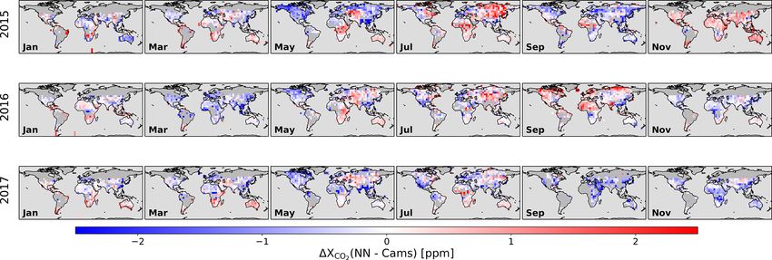
120 L. David et al.: A neural network approach for XCO2 retrieval
except when these are successive in the typical ranking. The on a prior performance analysis. We have analyzed how the
procedure described here fills the missing elements and the performance of the NN approach varies with the quality in-
NN can then be applied to the corrected spectrum to estimate dicators. For this objective, we have compared the retrieved
the surface pressure and XCO2 . surface pressure against the value derived from the numer-
ical weather data, as in Fig. 1, and we have evaluated the
statistics of their difference as a function of the quality flags.
3 Results First (figure not shown), there is no significant difference be-
tween the cases when the measured spectra are complete and
Figure 1 shows a density histogram of the GEOS5 FP-IT sur- those when one or several missing pixel elements have been
face pressure analysis and of the NN estimate for the eval- interpolated with the method described above. Conversely,
uation dataset (odd-numbered months). Clearly, there is an the statistics vary with the cloud flag and the warn level, as
excellent agreement between the two over a very wide range shown in Fig. 3. We only use the spectra for which an ACOS
of surface pressures. There is no significant bias and the stan- retrieval is available. Among those, and according to the flag
dard deviation is 2.9 hPa. The equivalent ACOS V8r retrieval cloud_flag_idp, about 53 % are labeled as “very clear” while
shows a bias of 1.5 hPa and a standard deviation of 3.4 hPa, 43 % are “probably clear”. The statistics are slightly better
slightly larger than that of the NN approach. Note that the for the former than they are for the latter. Conversely, the
ACOS statistics are those of the ACOS retrieval–minus–prior rather rare “definitely cloudy” and “probably cloudy” show
statistics (see Sect. 2). Interpreting them in terms of error is deviations that are significantly larger. This result was highly
counterintuitive because the Bayesian retrieval is supposed to expected since our NN did not learn how to handle clouds
be better than the prior, but in practice radiation modeling er- in the spectra. Therefore, all “definitely cloudy” and “proba-
rors lead to a different interpretation (see, e.g., the discussion bly cloudy” soundings are outside the domain covered by the
in Sect. 4.3.4 of O’Dell et al., 2018). training dataset. Note also that the observations used here
Both NN and ACOS correlations with GEOS5 FP-IT are have all been classified as “clear” by ACOS preprocessing.
very high (0.997 and 0.996) although the best fit shows a very Thus, most OCO-2 observations are not used here and Fig. 3
small deviation from the 1 : 1 line. Interestingly, the best-fit should not be interpreted as the ability to retrieve the surface
deviations from the 1 : 1 line are of opposite sign (slopes 0.99 pressure in cloudy conditions. Most (78 %) of the observa-
and 1.01). The results of the NN are surprisingly good given tions have a warn level of 0. The deviation statistics increase
the simplicity of the approach and given that the NN estimate with the warn level, both in terms of bias and standard de-
does not use any a priori information or ancillary informa- viation. In comparison, the difference in the statistics for an
tion such as the surface altitude or temperature profile, con- outcome flag of 1 and 2 are small. Besides, more than half
trarily to the ACOS estimate. The quality of the NN results of the ACOS retrievals have an outcome flag of 2, which en-
for the estimate of the surface pressure is a first demonstra- courages us not to reject those for further use. Based on this
tion of the potential of the approach. Note that the retrieval analysis, we retain all spectra that are very clear (cloud flag
accuracy holds over a very large range of surface pressures of 2 or 3) and that have a warn level of 2 or less.
(the relative variations of XCO2 are much smaller), although We made a figure similar to Fig. 3 but based on the XCO2
there is some indication of biases for the lowest pressures that estimates (not shown). Although the results are similar in
are underrepresented in the training dataset. These biases of terms of sign (i.e., increase of the deviations with the warn
≈ 5 hPa affect the observations over high-elevation surfaces levels), the signal is not as obvious (there is less relative dif-
such as the Tibetan Plateau or the US Rocky Mountains. ference between one warn level and another, or for the vari-
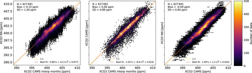
Figure 2 is similar to Fig. 1 but for XCO2 . There is no sig- ous cloud flags). Our interpretation is that the relative accu-
nificant bias between the NN estimate and the CAMS model, racy of the surface pressure used as a reference estimate is
while the standard deviation is 0.84 ppm. The bias-corrected much better than that of the NN retrieval, whereas the accu-
ACOS retrievals show a slight bias against the CAMS model racy of the XCO2 from CAMS is not much better than that
and the standard deviation (1.14 ppm) is larger than that of of the NN. As a consequence, variations in the accuracy of
the NN approach. Note that the statistics given here are af- the NN do not show up as clearly for XCO2 than they do for
fected by CAMS modeling errors that may eventually be cor- the surface pressure.
rected with the help of the satellite information. The best fit A standard method to evaluate an algorithm that estimates
slope deviations from the 1 : 1 line are larger than for the sur- XCO2 from spaceborne observation is the comparison of its
face pressure; the slopes are 0.93 for the NN and 0.87 for products against estimates from TCCON retrievals. These es-
ACOS. timates use ground-based solar absorption spectra recorded
Figures 1 and 2, together with the quantitative assessment by Fourier transform infrared spectroscopy and have been
of the precision, are given for the observations that are clear tuned with airborne in situ profiles (Wunch et al., 2010). To
according to ACOS (cloud flag = 2 or 3), that have a warn take advantage of the full potential of the TCCON retrievals
level of 2 or less, that may include missing pixel elements, for the bias correction and validation of the XCO2 estimates,
and that have an outcome flag of 1 or 2. This choice is based the OCO-2 platform can be oriented so that the instrument
Atmos. Meas. Tech., 14, 117–132, 2021 https://doi.org/10.5194/amt-14-117-2021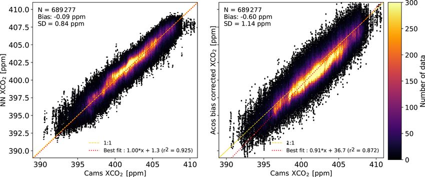
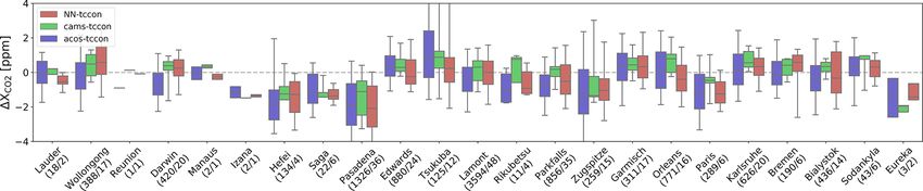
L. David et al.: A neural network approach for XCO2 retrieval                                                                               121

Figure 1. Density histogram of the surface pressure retrieved from the OCO-2 satellite measurements against those derived from GEOS-
FP-IT. Panel (a) is for the NN approach while panel (b) is for the ACOS V9r retrieval (using the official bias correction). The figure insets
provide the number of data points, the bias, the standard deviation, the equation of the best linear fit, and the correlation. The yellow line is
the 1 : 1 line whereas the red dotted line is the best linear fit.

Figure 2. Same as Fig. 1 but for XCO2 . In this case, the reference data are the CAMS v18r2 simulation.

field of view is close to the surface station. The ACOS full-              CAMS. The statistics per station are provided in Table 1.
physics algorithm can handle these spectra that are acquired               Two stations, Paris and Pasadena, show a large negative bias
in neither nadir nor glint geometries, but the NN was trained              for both estimates, which may be interpreted as the impact
solely on nadir spectra and cannot yet be applied to the ob-               of the city on the atmosphere sampled by the TCCON mea-
servations acquired in target mode. We thus have to rely on                surement, while the atmosphere sampled by the distant satel-
nadir measurements acquired in the vicinity of TCCON sites.                lite may be less affected. Conversely, there is no such neg-
In the following, we use nadir measurements that are within                ative bias for other stations that are located close to large
5◦ in longitude and 1.5◦ in latitude to the TCCON site. The                cities, such as Tsukuba, a suburb of the Tokyo Metropoli-
XCO2 estimates (either from ACOS, the NN, or the model                     tan area. Zugspitze is rather specific due to its high altitude.
sampled at the OCO-2 measurement location) are averaged                    The comparison against TCCON indicates that the NN ap-
for a given overpass. Similarly, we average the TCCON es-                  proach performs similarly to ACOS, if not better. The dis-
timates of XCO2 within 30 min of the satellite overpass. No                persion is larger for one approach versus the other for some
attempt was made to correct for the different weighting func-              stations, while the opposite is true for other stations. Note
tions of the surface and spaceborne remote sensing estimates.              also that the CAMS model performs better than both satellite
The comparisons are shown in Fig. 4 for each TCCON sta-                    retrievals for most stations. This observation provides further
tion listed in Table 1.                                                    justification to the use of this model for training the NN.
   Overall, the biases and standard deviations of the differ-                 The evaluation of the algorithm performance is limited by
ences to TCCON observations are −0.34 ± 1.40 ppm for the                   the distance between the satellite estimate and its surface val-
NN, −0.47 ± 1.49 ppm for ACOS and 0.04 ± 1.09 ppm for                      idation. This is inherent to the use of nadir-only observations

https://doi.org/10.5194/amt-14-117-2021                                                           Atmos. Meas. Tech., 14, 117–132, 2021
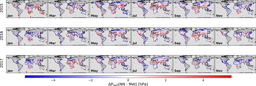
122                                                                L. David et al.: A neural network approach for XCO2 retrieval

Figure 3. Statistics on the difference between the surface pressure retrieved by the NN approach and those derived from the weather analyses
as a function of various quality parameters. In these figures, the red line is the median, the boxes indicate the 25 % and 75 % percentiles, and
the whiskers indicate the 5 %–95 % range. Panel (a) shows the statistics as a function of the cloud flag, panel (b) is as a function of the warn
level, while panel (c) is as a function of the outcome flag.

Figure 4. Statistics of the differences between the NN retrieval (red), the CAMS model (green) or the bias-corrected ACOS retrievals (blue),
and the TCCON retrievals. The boxes indicate the 25 %–75 % percentiles and the median is shown by the horizontal line within the box.
The whiskers indicate the 5 %–95 % percentiles. Stations are ordered by increasing latitudes. The numbers below the station name indicate
the number of individual observations and coincidence days used for the statistics. The references for the various TCCON observations are
provided in Table 1.

that are seldom located close to the TCCON sites. A reduc-                used for the training and therefore do not show any signifi-
tion of the distance results in less coincidences, which leads            cant differences. There are very clear spatial patterns of a few
to a validation dataset of poor representativeness. Note that             hPa that are not expected and should be interpreted as a bias
the CAMS model was sampled at the location of the satellite               in the NN approach. The biases over the high mountains and
observations, so that the higher performance of the model                 plateaus have already been mentioned. In addition, positive
versus the satellite products cannot be caused by a higher                biases tend to occur in the high latitudes and negative biases
proximity to the TCCON station.                                           toward the tropics. The structures show additional spatial and
   We now investigate whether the model–minus–NN differ-                  temporal patterns and are therefore more complex than just
ences are purely random or contain some spatial or tempo-                 a latitude function. The same figure but based on the ACOS
ral structures. This question is important because if the dif-            retrievals (Fig. A3) displays large-scale structures with dif-
ferences show a random structure there is little hope to use              ferent spatial patterns; the surface pressure bias is mostly
these data to improve the surface fluxes used in the CAMS                 negative over northern latitudes and positive over low lati-
product. Conversely, if the XCO2 differences do show some                 tudes. A histogram (Fig. 6) of the monthly differences, such
structures, they can be attributed to surface flux errors in              as those shown on Fig. 5, confirms that the amplitude of the
the CAMS product that may then be corrected through in-                   surface pressure biases is larger with ACOS than it is with the
verse atmospheric modeling. There is no certainty, however,               NN. The NN or ACOS surface pressure bias is −0.33 hPa or
as a spatial structure in the NN–minus–CAMS difference can                1.39 hPa, respectively, and the standard deviation is 2.12 or
also be interpreted as a bias in the satellite estimate.                  2.79 hPa, respectively.
   We first show (Fig. 5) the difference between the NN esti-                Figure 7 is similar to Fig. 5 but for XCO2 differences be-
mates of the surface pressure and the numerical weather anal-             tween the NN estimate and the CAMS model. As for the
yses. These are monthly maps of the NN-minus-CAMS dif-                    surface pressure, there are clear spatial patterns with ampli-
ference for 3 years of the period at a 5◦ × 5◦ resolution. We             tudes of 1 to 2 ppm. The question is whether these are mostly
only present the odd-numbered months as the others were                   linked to monthly biases in the CAMS model or to the NN.

Atmos. Meas. Tech., 14, 117–132, 2021                                                          https://doi.org/10.5194/amt-14-117-2021
L. David et al.: A neural network approach for XCO2 retrieval                                                                       123

Table 1. TCCON stations used in this paper (Fig. 4). The data were obtained from the http://tccondata.org website at during the summer of
2019 (last access: 1 August 2019).

       Stations               [lat; long]   Altitude   Reference                                   Biases                SD
                                                 [m]                                        NN/ACOS/CAM         NN/ACOS/CAM
       Lauder         [−45.04; 169.68]          370    Sherlock et al. (2017)            −0.48/−0.25/0.076         0.43/1.51/0.16
       Wollongong     [−34.41; 150.88]           30    Griffith et al. (2017b)              0.60/−0.20/0.42        1.21/1.32/0.60
       Reunion          [−20.90; 55.49]          90    De Maziere et al. (2017)           −0.08/−0.90/0.13                  –/–/–
       Darwin         [−12.43; 130.89]           30    Griffith et al. (2017a)              0.19/−0.69/0.23        0.80/1.09/0.72
       Manaus            [−3.21; −60.6]          50    Dubey et al. (2017)                −0.25/−0.05/0.34         0.43/1.04/0.26
       Izana              [28.3; −16.48]       2300    Blumenstock et al. (2017)         −1.35/−1.14/−1.48          0.18/0.92/0.0
       Hefei             [31.90; 118.67]         30    Liu et al. (2018)                 −1.47/−1.58/−1.01         1.11/1.76/0.63
       Saga              [33.24; 130.29]         10    Shiomi et al. (2017)              −1.36/−1.03/−1.15         0.57/1.22/0.59
       Pasadena       [34.14; −118.13]          240    Wennberg et al. (2017b)           −2.12/−1.87/−1.41         1.57/1.64/1.17
       Edwards        [34.96; −117.88]          700    Iraci et al. (2017)                    0.07/0.41/0.50       1.00/1.01/0.64
       Tsukuba           [36.05; 140.12]         30    Morino et al. (2017a)                  0.42/1.43/1.05       2.13/2.53/1.61
       Lamont             [36.6; −97.49]        320    Wennberg et al. (2017c)            −0.03/−0.38/0.16         1.07/1.21/0.94
       Rikubetsu       [43.46; 1473.77]         390    Morino et al. (2017b)              −0.57/−0.84/0.47         0.84/1.07/0.98
       Parkfalls        [45.94; −90.27]         440    Wennberg et al. (2017a)            −0.41/−0.75/0.11         1.15/1.01/0.72
       Zugspitze           [47.42; 11.06]      2960    Sussmann and Rettinger (2017b)    −0.85/−1.14/−0.83         1.45/1.85/1.36
       Garmisch            [47.48; 11.06]       740    Sussmann and Rettinger (2017a)         0.40/0.28/0.43       0.98/1.29/0.62
       Orleans              [47.97; 2.11]       130    Warneke et al. (2017)                −0.35/0.13/0.66        1.06/1.38/0.67
       Paris                [48.85; 2.36]        60    Te et al. (2017)                  −1.29/−1.24/−0.62         1.30/1.66/1.23
       Karlsruhe             [49.1; 8.44]       110    Hase et al. (2017)                     0.26/0.21/0.75       0.80/1.29/0.55
       Bremen               [53.10; 8.85]         7    Notholt et al. (2017)                0.30/−0.07/0.36        1.11/1.02/0.45
       Bialystok           [53.23; 23.02]       180    Deutscher et al. (2017)            −0.11/−0.32/0.33         1.31/1.30/0.42
       Sodankyla           [67.37; 26.63]       190    Kivi et al. (2017)                     0.26/0.24/0.61       0.79/1.36/0.80
       Eureka           [80.05; −86.42]         600    Strong et al. (2017)              −1.02/−1.50/−2.16         1.01/2.25/0.41

Figure 5. Difference between the NN estimates of the surface pressure and the numerical weather analyses. The differences have been
averaged at monthly and spatial 5◦ × 5◦ resolutions. The results are shown for 3 years and only for the months that were not used for the
training.

The first hypothesis is of course more favorable as it would           ther analysis, in particular atmospheric flux inversion, is nec-
indicate that the satellite data can bring new information to          essary for a proper interpretation of the NN–CAMS differ-
constrain the surface fluxes. However, the analysis of the sur-        ences.
face pressure that shows biases of several hPa suggests that              The differences of ACOS estimates to the CAMS model
the NN XCO2 estimate may also show biases with spatially               also show patterns of similar amplitude as those in Fig. 7
coherent patterns. Interestingly, the patterns vary in time and        (Fig. A4). However, there is no clear correspondence be-
are not correlated with those of the surface pressure. Fur-            tween these patterns and those obtained using the NN prod-

https://doi.org/10.5194/amt-14-117-2021                                                     Atmos. Meas. Tech., 14, 117–132, 2021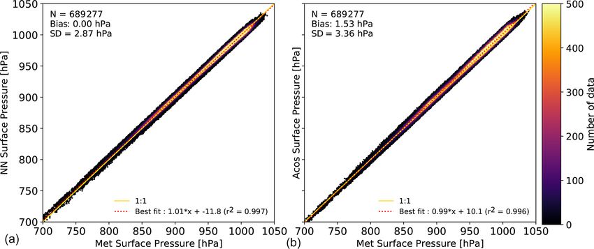
124                                                                L. David et al.: A neural network approach for XCO2 retrieval

                                                                        mation on the observation location and then generates an es-
                                                                        timate based on the corresponding CAMS value. However,
                                                                        since the observation geometry is exactly the same from one
                                                                        year to the next, there is no information, direct or indirect,
                                                                        on the observation year in the NN input. Thus, the XCO2
                                                                        growth rate that is accurately retrieved by the NN method
                                                                        (see Fig. 7) is necessarily derived from the spectra. A simi-
                                                                        lar argument can be made on the spatial variation across the
                                                                        longitudes.
                                                                           To further demonstrate that the NN retrieves XCO2 from
                                                                        the spectra rather than from the prior, we performed an ad-
                                                                        ditional experiment. The training is based only on even-
                                                                        numbered months. As a consequence, the prior does not in-
                                                                        clude any direct information on the odd-numbered months.
                                                                        For these months, the best prior estimate is a linear interpo-
                                                                        lation between the two adjacent even-numbered months. We
                                                                        can then analyze how the NN estimate compares with the
                                                                        CAMS product, which accounts for the true synoptic vari-
                                                                        ability, and a degraded version of CAMS based on a linear
                                                                        interpolation between the two adjacent months. This com-
Figure 6. Histogram of the monthly mean differences at 5◦ resolu-       parison is shown in Fig. 8. The center figure compares the
tion (such as those shown in Fig. 5) between the satellite retrievals   true CAMS value and that derived from the temporal inter-
and the CAMS model: (a) is for XCO2 while (b) is for the surface        polation. As expected, both are highly correlated (the sea-
pressure. The blue line is for the NN product while the orange line
                                                                        sonal cycle and the growth rate are kept in the interpolated
is for ACOS.
                                                                        values) but nevertheless show a difference standard devia-
                                                                        tion of 0.89 ppm. This value can be interpreted as the syn-
uct. The differences between the satellite products and the             optic variability of XCO2 present in CAMS but not captured
CAMS model are small, but these contain the information                 in the interpolated product. The comparison of the NN esti-
that may be used to improve our knowledge on the surface                mate against CAMS (right) and the interpolated CAMS (left)
fluxes. The absence of a clear correlation between the spa-             shows significantly better agreement to the former. Thus, the
tiotemporal pattern from the NN and ACOS approaches in-                 NN product reproduces some XCO2 variability that is not
dicate that their use would lead to very different corrections          contained in the training prior. It provides further demonstra-
on the surface fluxes if used as input of an atmospheric in-            tion that the NN estimates relies on the spectra rather than on
version approach. Figure 6a shows the histogram of these                the time/space variations of the training dataset.
monthly mean differences. The histograms are very similar                  The results shown above indicate that the NN approach
for the two satellite products, although the standard devia-            allows an estimate of surface pressure and XCO2 with a pre-
tion of the difference to the CAMS model is slightly larger             cision that is similar or better than that of the operational
for ACOS than it is for the NN approach (0.89 vs. 0.83 ppm).            ACOS algorithm. The lack of independent “truth” data does
                                                                        not allow a full quantification of the product precision and
                                                                        accuracy. However, there are indications that the accuracy on
4     Discussion and conclusion                                         the surface pressure is better than 3 hPa rms, while the pre-
                                                                        cision (standard deviation) of XCO2 is better than 0.9 ppm.
The use of the same product for the NN training and its eval-           The data used for the XCO2 product evaluation has its own
uation may be seen as a weakness of our analysis. One may               error that is difficult to disentangle from that of the estimate
argue that the NN has learned from the model and generates              based on the satellite observation. It may also contain a bias
an estimate (either the surface pressure or XCO2 ) that is not          that is propagated to the NN through its training.
based on the spectra but rather on some prior information.                 One obvious advantage of the NN approach is the speed of
Let us recall that the NN input does not contain any informa-           the computation, which is several orders of magnitude higher
tion on the location or date of the observation. This is a strong       than that of the full-physics algorithm. This is significant
indication that the information is derived from the spectra as          given the current reprocessing time of the OCO-2 dataset
the NN does not “know” the CAMS value that corresponds to               despite the considerable computing power made available
the observation location. Yet, the NN input also includes the           for the mission. It also bears interesting prospects for future
observation geometry (sun angle and azimuth) that is some-              XCO2 imaging missions that will bring even higher data vol-
what correlated with the latitude and day of the year. One              ume (e.g., Pinty et al., 2017).
may then argue that the NN learns from this indirect infor-

Atmos. Meas. Tech., 14, 117–132, 2021                                                     https://doi.org/10.5194/amt-14-117-2021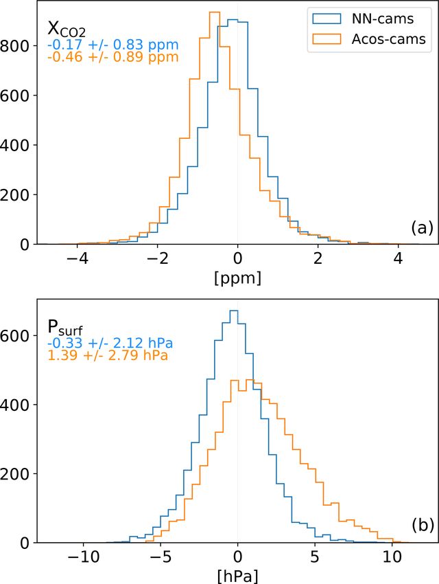
L. David et al.: A neural network approach for XCO2 retrieval                                                                       125

Figure 7. Same as Fig. 5 but for the difference between the XCO2 estimated by the NN approach and that derived from the CAMS model.

Figure 8. Scatterplots of XCO2 estimated by the NN, the CAMS model, and the CAMS model that has been interpolated in time from
adjacent months (see text for details). Note that the number of points is less than in Fig. 2 because the edge months could not always be
interpolated.

   Another advantage is that the NN approach described in              vector reports the sensitivity of the retrieved total column to
this paper does not require the extensive debias procedure             changes in the concentration profile (Connor et al., 1994).
necessary for the ACOS product (O’Dell et al., 2018; Kiel et           It is a combination of physical information (about radiative
al., 2019). Per construction, there is no bias between the NN          transfer) and statistical information (about the prior infor-
estimates and the dataset used for the NN training. The NN             mation). It is needed for a proper comparison with 3D at-
approach therefore requires less effort and fewer resources.           mospheric models (e.g., Chevallier, 2015). When comparing
   There are, however, a number of drawbacks for the NN                with model simulations, for instance for atmospheric inver-
approach described in this paper.                                      sion, we may wish to neglect the NN implicit prior infor-
   One obvious drawback is the use of a CO2 model simula-              mation. This hypothesis leads to a homogeneous pressure
tion in the training while the main purpose of the satellite ob-       weighting over the vertical, as this is the product that the NN
servation is to improve our current knowledge of atmospheric           was trained to simulate. Alternatively, we could decide to ne-
CO2 and its surface fluxes. Our argument is that although the          glect the difference in prior information between the NN and
CAMS simulation used here has high skill (as demonstrated              the full-physics algorithm and use typical averaging kernels
in Fig. 4), it may have positive or negative XCO2 biases for           of the latter. A third, more involved option would be to per-
some months and some areas. These biases are independent               form a detailed sensitivity study of the NN, based on radia-
from the measured spectra so that the NN training will aim at          tive transfer simulations.
average values. As a consequence, the NN product could in                 Similarly, the current version of our neural network does
principle be of higher quality than the CAMS product, even             not provide a posterior uncertainty. A Monte Carlo approach
though the same model has been used as the reference esti-             using various training datasets could be use in the future for
mate for the training (see, e.g., Aires et al., 2005).                 such an estimate.
   Another drawback of the NN approach is that it does not                Also, because of the CO2 growth rate, the developed NN
directly provide its averaging kernel. The averaging kernel            cannot be safely used to process observations that are ac-

https://doi.org/10.5194/amt-14-117-2021                                                     Atmos. Meas. Tech., 14, 117–132, 2021
126                                                          L. David et al.: A neural network approach for XCO2 retrieval

quired later than a few weeks after the last data of the train-      Our next objective is to attempt a similar NN approach for
ing dataset, as the observed CO2 may then be outside of its       the measurements that were acquired in the glint mode. As
range. Therefore, the use of the neural network approach for      explained above, the glint observations may be more diffi-
near real-time applications would require frequent updates of     cult to reproduce by the NN than those acquired in the nadir
the training phase.                                               mode. However, we were very much surprised by the per-
   We acknowledge the fact that the NN product evaluated          formance of the NN with the nadir data and cannot preclude
here is not fully independent from the ACOS product. In-          being surprised again. Finally, we shall analyze the spatial
deed, we use the cloud flag and the quality diagnostic from       structure of the NN retrievals in regions that are expected to
ACOS to select the spectra that are of sufficient quality. If     be homogeneous and in regions where structures of anthro-
we aim for some kind of operational product, there is a need      pogenic origin are expected (e.g., Nassar et al., 2017; Reuter
to design a procedure to identify these good quality spec-        et al., 2019).
tra. One option would be to compare the surface pressure
retrieved by the NN to the numerical weather analysis es-
timate and to reject cases with significant deviations (e.g.,
differences larger than 3 hPa).
   Despite these drawbacks, the results presented here show
that a neural network has a large potential for the estimate of
XCO2 from satellite observations, such as those from OCO-
2, the forthcoming MicroCarb (Pascal et al., 2017), or the
CO2 M constellation (Sierk et al., 2018), which aims to mea-
sure anthropogenic emissions. It is rather amazing that a first
attempt leads to trueness and precision numbers that are sim-
ilar or better than those of the full-physics algorithm. There
are several paths to improvement. One is to provide the NN
with some ancillary information such as the surface altitude
or a proxy of the atmospheric temperature. Another is to train
the NN with model estimates (such as those of CAMS used
here) but that have been better sampled for their assumed pre-
cision, for instance through a multimodel evaluation. Also,
one could train the NN with observations acquired during
a few days of each month, rather than the even-numbered
months as done here, so that the evaluation dataset would
provide a better evaluation of the seasonal cycle.

Atmos. Meas. Tech., 14, 117–132, 2021                                               https://doi.org/10.5194/amt-14-117-2021
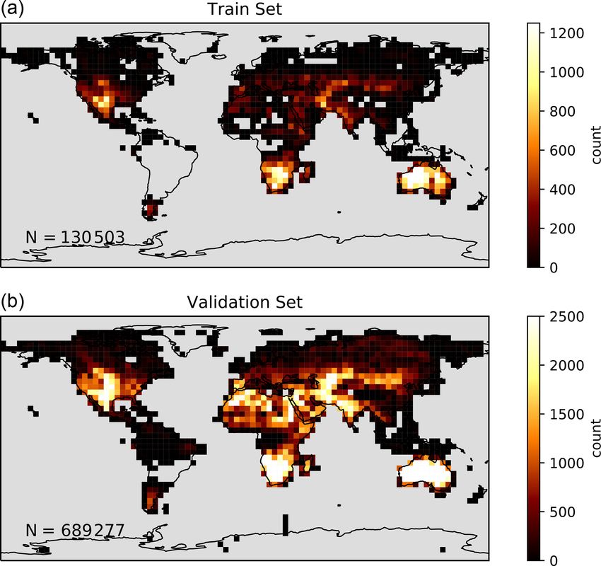
L. David et al.: A neural network approach for XCO2 retrieval                                                                           127

Appendix A

Figure A1. Illustration of the iterative convergence of the NN during its training. The loss is an indicator of the difference between the
NN estimate and the dataset. One dataset is used for the best estimate of the NN weights whereas another independent one is used for the
evaluation of the NN capability. The NN is stopped when there is no further reduction of the loss for the test dataset for 50 iterations. The
weights for the NN are those obtained for the lowest loss of the test dataset (iteration 167 on the figure).

Figure A2. Spatial density of the observations that were used for the training (a) and validation (b) processes.

https://doi.org/10.5194/amt-14-117-2021                                                         Atmos. Meas. Tech., 14, 117–132, 2021
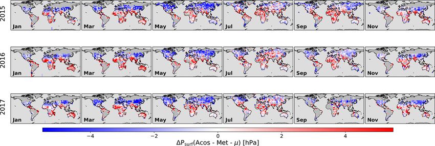
128                                                             L. David et al.: A neural network approach for XCO2 retrieval

Figure A3. Same as Fig. 5 but for the surface pressure retrieved by the ACOS algorithm. The mean bias over the full period (µ) is removed
so that the differences are centered on zero.

Figure A4. Same as Fig. 7 but for the XCO2 retrieved by the ACOS algorithm. The mean bias over the full period (µ) is removed so that the
differences are centered on zero.

Atmos. Meas. Tech., 14, 117–132, 2021                                                     https://doi.org/10.5194/amt-14-117-2021
L. David et al.: A neural network approach for XCO2 retrieval                                                                           129

Code and data availability. The code used in this paper and the          Plenary/32/documents/CEOS_AC-VC_White_Paper_Version_
CAMS model simulations are available, upon request, from the au-         1_20181009.pdf (last access: 18 October 2019), 2018.
thor. The OCO-2 and TCCON data can be downloaded from their            Chédin, A., Serrar, S., Scott, N. A., Crévoisier, C., and Armante R.:
respective websites. The TCCON data is available from the web-           First global measurement of midtropospheric CO2 from NOAA
site http://tccondata.org (TCCON, 2021), whereas the OCO-2 data          polar satellites: Tropical zone, J. Geophys. Res., 108, 4581,
is available from http://ocov2.jpl.nasa.gov (NASA Jet Propulsion         https://doi.org/10.1029/2003JD003439, 2003.
Laboratory, 2021).                                                     Chevallier, F.: On the statistical optimality of CO2 atmospheric
                                                                         inversions assimilating CO2 column retrievals, Atmos. Chem.
                                                                         Phys., 15, 11133–11145, https://doi.org/10.5194/acp-15-11133-
Author contributions. FMB designed the study. LD developed the           2015, 2015.
code and performed the computations. All authors shared the result     Chevallier, F., Fisher, M., Peylin, P., Serrar, S., Bousquet, P.,
analysis.                                                                Bréon, F.-M., Chédin, A., and Ciais, P.: Inferring CO2 sources
                                                                         and sinks from satellite observations: Method and appli-
                                                                         cation to TOVS data, J. Geophys. Res., 110, D24309,
Competing interests. The authors declare that they have no conflict      https://doi.org/10.1029/2005JD006390, 2005.
of interest.                                                           Chevallier, F., Ciais, P., Conway, T. J., Aalto, T., Anderson, B. E.,
                                                                         Bousquet, P., Brunke, E. G., Ciattaglia, L., Esaki, Y., Frohlich,
                                                                         M., Gomez, A., Gomez-Pelaez, A. J., Haszpra, L., Krummel, P.
                                                                         B., Langenfelds, R. L., Leuenberger, M., Machida, T., Maignan,
Acknowledgements. OCO-2 L1 and L2 data were produced by the
                                                                         F., Matsueda, H., Morgu, J. A., Mukai, H., Nakazawa, T., Peylin,
OCO-2 project at the Jet Propulsion Laboratory, California Institute
                                                                         P., Ramonet, M., Rivier, L., Sawa, Y., Schmidt, M., Steele, L. P.,
of Technology, and obtained from the ACOS/OCO-2 data archive
                                                                         Vay, S. A., Vermeulen, A. T., Wofsy, S., and Worthy, D.: CO2 sur-
maintained at the NASA Goddard Earth Science Data and Informa-
                                                                         face fluxes at grid point scale estimated from a global 21 year re-
tion Services Center. TCCON data were obtained from the TCCON
                                                                         analysis of atmospheric measurements, J. Geophys. Res.-Atmos.,
Data Archive (http://tccondata.org, last access: 5 January 2021). We
                                                                         115, D21307, https://doi.org/10.1029/2010JD013887, 2010.
warmly thank those who made these data available.
                                                                       Connor, B. J., Siskind, D. E., Tsou, J. J., Parrish, A., and Remsberg,
                                                                         E. E.: Ground-based microwave observations of ozone in the up-
                                                                         per stratosphere and mesosphere, J. Geophys. Res., 99, 16757–
Financial support. This work was in part funded by CNES, the             16770, 1994.
French space agency, in the context of the preparation for the Mi-     Crisp, D., Atlas, R. M., Breon, F.-M., Brown, L. R., Burrows, J.
croCarb mission.                                                         P., Ciais, P., Connor, B. J., Doney, S. C., Fung, I. Y., Jacob,
                                                                         D. J., Miller, C. E., O’Brien, D., Pawson, S., Randerson, J. T.,
                                                                         Rayner, P., Salawitch, R. J., Sander, S. P., Sen, B., Stephens,
Review statement. This paper was edited by Piet Stammes and re-          G. L., Tans, P. P., Toon, G. C., Wennberg, P. O., Wofsy, S. C.,
viewed by Christopher O’Dell and one anonymous referee.                  Yung, Y. L., Kuang, Z., Chudasama, B., Sprague, G., Weiss,
                                                                         B., Pollock, R., Kenyon, D., and Schroll, S.: The Orbiting Car-
                                                                         bon Observatory (OCO) mission, Adv. Space Res., 34, 700–709,
                                                                         https://doi.org/10.1016/j.asr.2003.08.062, 2004.
                                                                       Crisp, D., Fisher, B. M., O’Dell, C., Frankenberg, C., Basilio, R.,
References                                                               Bösch, H., Brown, L. R., Castano, R., Connor, B., Deutscher,
                                                                         N. M., Eldering, A., Griffith, D., Gunson, M., Kuze, A., Man-
Agustí-Panareda, A., Diamantakis, M., Massart, S., Chevallier, F.,       drake, L., McDuffie, J., Messerschmidt, J., Miller, C. E., Morino,
  Muñoz-Sabater, J., Barré, J., Curcoll, R., Engelen, R., Lange-         I., Natraj, V., Notholt, J., O’Brien, D. M., Oyafuso, F., Polonsky,
  rock, B., Law, R. M., Loh, Z., Morguí, J. A., Parrington,              I., Robinson, J., Salawitch, R., Sherlock, V., Smyth, M., Suto,
  M., Peuch, V.-H., Ramonet, M., Roehl, C., Vermeulen, A. T.,            H., Taylor, T. E., Thompson, D. R., Wennberg, P. O., Wunch, D.,
  Warneke, T., and Wunch, D.: Modelling CO2 weather – why hor-           and Yung, Y. L.: The ACOS CO2 retrieval algorithm – Part II:
  izontal resolution matters, Atmos. Chem. Phys., 19, 7347–7376,         Global XCO2 data characterization, Atmos. Meas. Tech., 5, 687–
  https://doi.org/10.5194/acp-19-7347-2019, 2019.                        707, https://doi.org/10.5194/amt-5-687-2012, 2012.
Aires, F., Prigent, C., and Rossow, W. B.: Sensitivity of satellite    De Maziere, M., Sha, M. K., Desmet, F., Hermans, C.,
  microwave and infrared observations to soil moisture at a global       Scolas, F., Kumps, N., Metzger, J.-M., Duflot, V., and
  scale: 2. Global statistical relationships, J. Geophys. Res., 110,     Cammas, J.-P.: TCCON data from Reunion Island (RE),
  D11103, https://doi.org/10.1029/2004JD005087, 2005.                    Release GGG2014R0, TCCON data archive, CDIAC,
Blumenstock, T., Hase, F., Schneider, M., Garcia, O. E.,                 https://doi.org/10.14291/tccon.ggg2014.reunion01.R1, 2017.
  and Sepulveda, E.: TCCON data from Izana (ES), Re-                   Deutscher, N. M., Notholt, J., Messerschmidt, J., Weinzierl,
  lease GGG2014R1, TCCON data archive, CDIAC,                            C., Warneke, T., Petri, C., Grupe, P., and Katryn-
  https://doi.org/10.14291/tccon.ggg2014.izana01.R1, 2017.               ski, K.: TCCON data form Bialystok (PL), Re-
CEOS: A Constellation Architecture for Monitoring Carbon                 lease GGG2014R2, TCCON data archive, CDIAC,
  Dioxide and Methane from Space, Technical Report, Uni-                 https://doi.org/10.14291/tccon.ggg2014.bialystok01.R2, 2017.
  versity of Zurich, Switzerland, Department of Informatics,
  available at: http://ceos.org/document_management/Meetings/

https://doi.org/10.5194/amt-14-117-2021                                                      Atmos. Meas. Tech., 14, 117–132, 2021
130 L. David et al.: A neural network approach for XCO2 retrieval Dubey, M., Henderson, B., Green, D., Butterfield, Z., Keppel- lease GGG2014R1, TCCON data archive, CDIAC, Aleks, G., Allen, N., Blavier, J.-F., Roehl, C., Wunch, D., https://doi.org/10.14291/tccon.ggg2014.karlsruhe01.R1/1182416, and Lindenmaier, R.: TCCON data from Manaus (BR), 2017. Release GGG2014R0, TCCON data archive, CDIAC, Iraci, L. T., Podolske, J., Hillyard, P. W., Roehl, C., Wennberg, https://doi.org/10.14291/tccon.ggg2014.manaus01.R0/1149274, P. O., Blavier, J.-F., Landeros, J., Allen, N., Wunch, D., 2017. Zavaleta, J., Quigley, E., Osterman, G., Albertson, R., Dun- Eldering, A., Pollock, R., Lee, R. A. M., Rosenberg, R., Oy- woody, K., and Boyden, H.: TCCON data from Edwards afuso, F., Crisp, D., Chapsky, L., and Granat, R.: Orbiting (US), Release GGG2014R1, TCCON data archive, CDIAC, Carbon Observatory (OCO) – 2 Level 1B Theoretical Ba- https://doi.org/10.14291/tccon.ggg2014.edwards01.R1/1255068, sis Document, available at: http://disc.sci.gsfc.nasa.gov/OCO-2/ 2017. documentation/oco-2-v7/OCO_2_L1B_ATBD.V7.pdf (last ac- Keras Team: Keras, available at: https://github.com/fchollet/keras cess: 16 June 2016), 2015. (last access: 5 January 2021), GitHub, 2015. Eldering, A., Wennberg, P. O., Crisp, D., Schimel, D., Gunson, Kiel, M., O’Dell, C. W., Fisher, B., Eldering, A., Nassar, R., M. R., Chatterjee, A., Liu, J., Schwandner, F. M., Sun, Y., MacDonald, C. G., and Wennberg, P. O.: How bias correction O’Dell, C. W., Frankenberg, C., Taylor, T., Fisher, B., Oster- goes wrong: measurement of XCO2 affected by erroneous sur- man, G. B., Wunch, D., Hakkarainen, J., Tamminen, J., and Weir, face pressure estimates, Atmos. Meas. Tech., 12, 2241–2259, B.: The Orbiting Carbon Observatory-2 early science investiga- https://doi.org/10.5194/amt-12-2241-2019, 2019. tions of regional carbon dioxide fluxes, Science, 358, eaam5745, Kivi, R., Heikkinen, P., and Kyrö, E.: TCCON data from Sodankyla https://doi.org/10.1126/science.aam5745, 2017. (FI), Release GGG2014R0, TCCON data archive, CDIAC, Friedlingstein, P., Jones, M. W., O’Sullivan, M., Andrew, R. M., https://doi.org/10.14291/tccon.ggg2014.sodankyla01.R0/1149280, Hauck, J., Peters, G. P., Peters, W., Pongratz, J., Sitch, S., Le 2017. Quéré, C., Bakker, D. C. E., Canadell, J. G., Ciais, P., Jack- Knorr, W.: Is the airborne fraction of anthropogenic CO2 son, R. B., Anthoni, P., Barbero, L., Bastos, A., Bastrikov, V., emissions increasing?, Geophys. Res. Lett., 36, L21710, Becker, M., Bopp, L., Buitenhuis, E., Chandra, N., Chevallier, https://doi.org/10.1029/2009GL040613, 2009. F., Chini, L. P., Currie, K. I., Feely, R. A., Gehlen, M., Gilfillan, Liu, C., Wang, W., and Sun, Y.: TCCON data from Hefei D., Gkritzalis, T., Goll, D. S., Gruber, N., Gutekunst, S., Har- (PCR), Release GGG2014R0, TCCON data archive, CDIAC, ris, I., Haverd, V., Houghton, R. A., Hurtt, G., Ilyina, T., Jain, https://doi.org/10.14291/tccon.ggg2014.hefei01.R0, 2018. A. K., Joetzjer, E., Kaplan, J. O., Kato, E., Klein Goldewijk, K., Lucchesi, R.: File Specification for GEOS-5 FP-IT (Forward Korsbakken, J. I., Landschützer, P., Lauvset, S. K., Lefèvre, N., Processing for Instrument Teams), Technical Report, NASA Lenton, A., Lienert, S., Lombardozzi, D., Marland, G., McGuire, Goddard Spaceflight Center, Greenbelt, MD, USA, avail- P. C., Melton, J. R., Metzl, N., Munro, D. R., Nabel, J. E. M. S., able at: https://ntrs.nasa.gov/archive/nasa/casi.ntrs.nasa.gov/ Nakaoka, S.-I., Neill, C., Omar, A. M., Ono, T., Peregon, A., 20150001438.pdf (last access: 4 December 2018), 2013. Pierrot, D., Poulter, B., Rehder, G., Resplandy, L., Robertson, E., Morino, I., Matsuzaki, T., and Shishime, A.: TC- Rödenbeck, C., Séférian, R., Schwinger, J., Smith, N., Tans, P. P., CON data from Tsukuba (JP), 125HR, Release Tian, H., Tilbrook, B., Tubiello, F. N., van der Werf, G. R., Wilt- GGG2014R2, TCCON data archive, CDIAC, shire, A. J., and Zaehle, S.: Global Carbon Budget 2019, Earth https://doi.org/10.14291/tccon.ggg2014.tsukuba02.R2, 2017a. Syst. Sci. Data, 11, 1783–1838, https://doi.org/10.5194/essd-11- Morino, I., Yokozeki, N., Matzuzaki, T., and Shishime, 1783-2019, 2019. A.: TCCON data from Rikubetsu (JP), Release Griffith, D. W., Deutscher, N. M., Velazco, V. A., Wennberg, P. GGG2014R2, TCCON data archive, CDIAC, O., Yavin, Y., Aleks, G. K., Washenfelder, R. A., Toon, G. C., https://doi.org/10.14291/tccon.ggg2014.rikubetsu01.R2, 2017b. Blavier, J.-F., Murphy, C., Jones, N., Kettlewell, G., Connor, NASA Jet Propulsion Laboratory: Orbiting Carbon Observatory- B. J., Macatangay, R., Roehl, C., Ryczek, M., Glowacki, 2, available at: http://ocov2.jpl.nasa.gov, last access: 5 Jan- J., Culgan, T., and Bryant, G.: TCCON data from Darwin uary 2021. (AU), Release GGG2014R0, TCCON data archive, CDIAC, Nassar, R., Hill, T. G., McLinden, C. A., Wunch, D., Jones, https://doi.org/10.14291/tccon.ggg2014.darwin01.R0/1149290, D., and Crisp, D.: Quantifying CO2 emissions from individual 2017a. power plants from space, Geophys. Res. Lett., 44, 10045–10053, Griffith, D. W., Velazco, V. A., Deutscher, N. M., Murphy, C., https://doi.org/10.1002/2017GL074702, 2017. Jones, N., Wilson, S., Macatangay, R., Kettlewell, G., Buchholz, Notholt, J., Petri, C., Warneke, T., Deutscher, N. M., R. R., and Riggenbach, M.: TCCON data from Wollongong Buschmann, M., Weinzierl, C., Macatangay, R., and (AU), Release GGG2014R0, TCCON data archive, CDIAC, Grupe, P.: TCCON data from Bremen (DE), Re- https://doi.org/10.14291/tccon.ggg2014.wollongong01.R0/1149291, lease GGG2014R0, TCCON data archive, CDIAC, 2017b. https://doi.org/10.14291/tccon.ggg2014.bremen01.R0/1149275, Hadji-Lazaro, J., Clerbaux, C., and Thiria, S.: An inversion algo- 2017. rithm using neural networks to retrieve atmospheric CO total O’Brien, D. M. and Rayner, P. J.: Global observations of the car- columns from high-resolution nadir radiances, J. Geophys. Res., bon budget 2. CO2 column from differential absorption of re- 104, 23841–23854, https://doi.org/10.1029/1999JD900431, flected sunlight in the 1.61 µm band of CO2 , J. Geophys. Res., 1999. 107, ACH6-1, https://doi.org/10.1029/2001JD000617, 2002. Hase, F., Blumenstock, T., Dohe, S., Gross, J., and O’Dell, C. W., Eldering, A., Wennberg, P. O., Crisp, D., Gunson, Kiel, M.: TCCON data from Karlsruhe (DE), Re- M. R., Fisher, B., Frankenberg, C., Kiel, M., Lindqvist, H., Man- Atmos. Meas. Tech., 14, 117–132, 2021 https://doi.org/10.5194/amt-14-117-2021
You can also read