Geophysical constraints on the properties of a subglacial lake in northwest Greenland
←
→
Page content transcription
If your browser does not render page correctly, please read the page content below
The Cryosphere, 15, 3279–3291, 2021
https://doi.org/10.5194/tc-15-3279-2021
© Author(s) 2021. This work is distributed under
the Creative Commons Attribution 4.0 License.

Geophysical constraints on the properties of a subglacial lake in
northwest Greenland
Ross Maguire1,2 , Nicholas Schmerr1 , Erin Pettit3 , Kiya Riverman4 , Christyna Gardner5 , Daniella N. DellaGiustina6 ,
Brad Avenson7 , Natalie Wagner8 , Angela G. Marusiak1 , Namrah Habib6 , Juliette I. Broadbeck6 , Veronica J. Bray6 ,
and Samuel H. Bailey6
1 Department  of Geology, University of Maryland, College Park, MD 20742, USA
2 Department  of Earth and Planetary Sciences, University of New Mexico, Albuquerque, NM 87131, USA
3 College of Earth, Ocean, and Atmospheric Sciences, Oregon State University, Corvallis, OR 97331-5503, USA
4 Courant Institute of Mathematical Sciences, New York University, New York, NY 10012 USA
5 Department of Geosciences, Utah State University, Logan, UT 84322-4505, USA
6 Lunar and Planetary Laboratory, University of Arizona, Tucson, AZ 85721-0092, USA
7 Silicon Audio Inc., Austin, Pflugerville, TX 78660, USA
8 Department of Geosciences, University of Alaska, Fairbanks, AK 99775, USA

Correspondence: Ross Maguire (rmaguire@umd.edu)

Received: 30 October 2020 – Discussion started: 13 November 2020
Revised: 10 May 2021 – Accepted: 11 May 2021 – Published: 16 July 2021

Abstract. In this study, we report the results of an active-       mechanisms of subglacial lake formation, evolution, and rel-
source seismology and ground-penetrating radar survey per-         ative importance to glacial hydrology.
formed in northwestern Greenland at a site where the pres-
ence of a subglacial lake beneath the accumulation area has
previously been proposed. Both seismic and radar results
show a flat reflector approximately 830–845 m below the sur-
face, with a seismic reflection coefficient of −0.43 ± 0.17,       1   Introduction
which is consistent with the acoustic impedance contrast be-
tween a layer of water and glacial ice. Additionally, in the       There is mounting evidence that subglacial lake systems be-
seismic data we observe an intermittent lake bottom reflec-        low the Antarctic and Greenland ice sheets play an important
tion arriving between 14–20 ms after the lake top reflection,      role in glacier dynamics and ice-sheet mass balance consid-
corresponding to a lake depth of approximately 10–15 m.            erations. In Antarctica, the presence of subglacial lakes is
A strong coda following the lake top and lake bottom re-           suspected to promote ice flow by reducing basal shear stress
flections is consistent with a package of lake bottom sedi-        (e.g., Bell et al., 2007), and periodic drainage events have
ments although its thickness and material properties are un-       been linked to accelerated ice flow in outlet glaciers and ice
certain. Finally, we use these results to conduct a first-order    streams (e.g., Stearns et al., 2008; Siegfried et al., 2016).
assessment of the lake origins using a one-dimensional ther-       Similarly, in Greenland subglacial lake systems also provide
mal model and hydropotential modeling based on published           a reservoir for the storage of surface or basal meltwater and
surface and bed topography. Using these analyses, we nar-          hence may be an important, but largely unknown, factor in
row the lake origin hypotheses to either anomalously high          global sea level change. Additionally, subglacial lakes are
geothermal flux or hypersalinity due to local ancient evap-        of interest due to their ability to harbor complex microor-
orite. Because the origins are still unclear, this site provides   ganisms adapted to extreme environments (Achberger et al.,
an intriguing opportunity for the first in situ sampling of a      2016; Campen et al., 2019; Vick-Majors et al., 2016) and
subglacial lake in Greenland, which could better constrain         paleoenvironmental information contained in subglacial lake
                                                                   sediments (Bentley et al., 2011).

Published by Copernicus Publications on behalf of the European Geosciences Union.
3280                                       R. Maguire et al.: Geophysical constraints on the properties of a subglacial lake

   While the presence and nature of subglacial lakes under-        which can provide valuable clues to their formation and to-
lying the Antarctic ice sheet has been studied for more than       tal volume. For example, Peters et al. (2008) performed an
50 years, the existence of subglacial lakes below the Green-       active-source seismic survey near the South Pole region of
land ice sheet is a relatively recent discovery and compara-       Antarctica and observed reflections from both the top and
tively little is known about their properties and origin. De-      bottom of a subglacial lake that lies 2.8 km below the ice
tection of subglacial lakes has relied on a variety of methods,    surface, which allowed them to image a lake depth of about
including radio-echo sounding (Robin et al., 1970; Siegert et      32 m and infer the underlying sedimentary structure. Addi-
al., 1996; Langley et al., 2011; Palmer et al., 2013; Young et     tionally, Woodward et al. (2010) performed an active-source
al., 2016; Bowling et al., 2019), satellite altimetry measure-     seismic investigation of Lake Ellsworth in west Antarctica,
ments (Fricker et al., 2007; Palmer et al., 2015; Siegfried and    which lies at the bottom of a narrow subglacial valley below
Fricker, 2018; Willis et al., 2015), and active-source seismic     approximately 3 km of ice. They found large variations in
experiments (e.g., Horgan et al., 2012; Peters et al., 2008).      lake depth from between 52 and 156 m and were able to es-
Using these techniques, approximately 400 subglacial lakes         timate the total volume of liquid water to be 1.37 km3 . Later,
have been detected in Antarctica (Wright and Siegert, 2012),       Smith et al. (2018) reanalyzed the data to investigate the sed-
of which 124 are considered “active” by Smith et al. (2009).       imentary structure below Lake Ellsworth and found evidence
In Greenland, subglacial lakes were first detected in radio-       of a thin sedimentary package (minimum thickness of 6 m),
echo sounding data by Palmer et al. (2013), who identi-            which they suggest may have built up slowly over at least
fied two small (roughly 10 km2 ) flat regions of anomalously       150 kyr. This contrasts to results from seismic investigations
high basal reflectivity below the northwestern Greenland ice       of Lake Vostok, the largest of Antarctica’s subglacial lakes,
sheet. These features, named L1 and L2, were discovered            which show evidence for a much thicker water column (up to
below 757 and 809 m of ice, respectively. Recently, Bowl-          1100 m) and a thicker layer of lake bottom sediments (up to
ing et al. (2019) greatly expanded the inventory of subglacial     400 m) below approximately 4 km of ice (e.g., Filina et al.,
lakes in Greenland to approximately 54 candidates based on         2008). Seismic investigations have also been useful for illu-
a combination of airborne radio-echo sounding and satellite        minating the properties of subglacial lakes below much thin-
altimetry data. The new inventory shows that, in contrast          ner ice columns in active ice streams, such as the subglacial
to subglacial lakes in Antarctica which tend to form under         Lake Whillans which is situated below approximately 800 m
thick (> 4 km) warm-based ice in the continental interior,         of ice and has a maximum water column thickness of less
the majority of subglacial lakes in Greenland are found un-        than 10 m (e.g., Horgan et al., 2012).
der relatively thin (1–2 km) ice near the margins of the ice
sheet. Bowling et al. (2019) find that most subglacial lakes in
Greenland appear to be stable features, showing temporally         2     Methods
consistent radio-echo sounding signatures and an absence of
vertical surface deformation over the decadal timescales of        2.1    Field experiment
observation. Of the 54 candidate lakes, only 2 showed signs
of vertical surface deformation indicative of active draining      In June 2018, we conducted a geophysical survey in north-
or recharge.                                                       western Greenland above the candidate subglacial lake
   The formation and location of the detected subglacial lake      feature named L2 by Palmer et al. (2013). This feature
features in Greenland remains elusive because many are lo-         sits within a 980 km2 drainage basin, is roughly adjacent
cated in regions where observations and modeling suggest           (< 10 km) to the nearest ice divide (Fig. 1a and b), and is
that the base of the ice is frozen to its bed (MacGregor et        within an accumulation area. Using RACMO2 1 km resolu-
al., 2016). Complicating our understanding of the nature of        tion modeling of Greenland’s near-surface climate and sur-
subglacial lakes is the fact that uniquely identifying lakes in    face mass balance (Noël et al., 2018), we estimate the mean
radar data is challenging since basal reflectivity is sensitive    annual air temperature to be −22 ◦ C. This model is forced
to both the physical properties and the roughness of the mate-     with ERA-Interim reanalysis climate information (Dee et al.,
rial underlying the ice (e.g., Jordan et al., 2017). Amplitude     2011) at the boundaries and evaluated with in situ observa-
anomalies of radar echoes in the range of +10 to +20 dB            tions. The mean annual snow accumulation rate at the field
are often interpreted as subglacial lakes, although flat regions   site is ∼ 0.3 m yr−1 ice equivalent. In order to confirm the
of saturated sediment may produce similar anomalies. Fur-          presence of the subglacial lake and investigate its physical
thermore, the total volume of water stored in subglacial lake      properties, we collected data using both active-source seis-
systems is unknown since airborne and space-based remote           mology and ground-penetrating radio-echo sounding (GPR).
sensing observations are incapable of measuring lake depth            The active-source seismic experiment (Fig. 1c) consisted
(i.e., water column thickness).                                    of a moving line of twenty-four 40 Hz vertical component
   Seismic investigations provide an independent means of          geophones spaced 5 m apart. For each line, we collected data
confirming the presence of subglacial lakes and are capable        at four shot locations using an 8 kg sledgehammer impacted
of measuring lake depth and underlying geological structures       against a 1.5 cm thick steel plate. At each source location

The Cryosphere, 15, 3279–3291, 2021                                                   https://doi.org/10.5194/tc-15-3279-2021
R. Maguire et al.: Geophysical constraints on the properties of a subglacial lake                                                       3281

Figure 1. (a) Map of Greenland showing our field location in the northwest. (b) Composite satellite image from Landsat 8 taken between
20 May 2018 and 27 May 2018. (c) Close-up map of field region. The green stars show the active-source shot, and the orange line shows the
track of the GPR survey. Only the first of four shot locations for each geophone line is plotted. (d) Geometry of the active-source experiment
for a single geophone line. The black lines indicate the raypaths of R1 between all source locations (stars) and geophones (red triangles).

at least five hammer shots were stacked into a single shot               plying a normal moveout (NMO) correction with a velocity
gather in order to increase the signal-to-noise ratio. The first         of 3700 m s−1 , which was found to be the average velocity of
shot location of each line was offset 115 m from the first               the ice column from NMO analysis of the primary bed reflec-
geophone, and subsequent shot locations were moved 115 m                 tion. High-frequency spatial noise with wavenumbers greater
along the line. After data were collected for each of the four           than 0.05 m−1 was removed with f-k filtering. Shot gathers
shot locations, the line was moved 230 m east along the tra-             with offsets of −115 and 230 m from the first geophone con-
verse and data collection was repeated. The seismic line was             tained an air wave arrival that was muted by zeroing a 10 ms
moved a total of 10 times, totalling 40 separate shot lo-                window with a moveout of 315 m s−1 .
cations. Using this geometry, we obtained reflection points                 The GPR data were collected across a ∼ 5.5 km transect
at the ice bottom spaced every 2.5 m along a traverse to-                roughly parallel to the seismic survey (Fig. 1c), using an ac-
talling 2400 m (Fig. 1d). We created a seismic reflection im-            quisition system especially adapted to be towed by a motor
age by bandpass-filtering data between 100–200 Hz and ap-                sled traveling at approximately 10 km h−1 (e.g., Welch and

https://doi.org/10.5194/tc-15-3279-2021                                                          The Cryosphere, 15, 3279–3291, 2021
3282                                        R. Maguire et al.: Geophysical constraints on the properties of a subglacial lake

Jacobel, 2003). The system used a Kentech pulse transmit-           reflection (e.g., Peters et al., 2008).
ter that produces ± 2000 V pulses with a variable pulse rep-
etition frequency of between 1 and 5 kHz. The antennae are                        AR2 (θ ) aL(θ)
                                                                    cR (θ ) = 2            e                                     (1)
resistively loaded wire dipoles with a nominal frequency of                       AR1 (θ )
5 MHz, and the receiver uses an 8 bit NI USB-5133 digitizer
                                                                    At a given geophone, two factors control the amplitude ra-
and a computer. We stacked 64 traces over a 10–15 m hor-
                                                                    tio between R1 and R2. First, R1 and R2 reflect off the
izontal distance, and then we filtered between 2–8 MHz in
                                                                    lake with slightly different angles, which changes the relative
postprocessing to produce each final trace on the radargram.
                                                                    amount of energy partitioned into each reflection. Second,
We created a GPR reflection image by converting the radar
                                                                    since R2 travels farther than R1, its amplitude is diminished
data to depth using a radar velocity of 172 m µs−1 (see Sup-
                                                                    due to geometrical spreading and attenuation. However, at
plement).
                                                                    incidence angles in this study, the difference in reflection co-
                                                                    efficients between R1 and R2 is negligible. Additionally, the
2.2    Basal radar reflectivity                                     path lengths of R1 and R2 vary by < 5 % between their short-
                                                                    est and farthest offsets. Therefore, to calculate the reflection
                                                                    coefficient cR , we use the normal incidence approximation
We estimated the relative basal reflectivity of the bed reflec-
                                                                    and compare amplitude ratios AR2 /AR1 on individual seis-
tor along the track by first correcting for geometric spread-
                                                                    mograms. In order to minimize the influence of the air wave
ing and then correcting for englacial attenuation assuming
                                                                    on AR2 /AR1 ratio, we exclude data from geophones with off-
the englacial attenuation rate is uniform. This assumption of
                                                                    sets between 135–155 m, where there is potential interfer-
uniform englacial attenuation is common (e.g., Christianson
                                                                    ence between R1 and the air wave. Measurements of AR1
et al., 2016; Palmer et al., 2013) but not ideal for this situ-
                                                                    and AR2 are made prior to f-k filtering.
ation because horizontal variability in the thermal structure
                                                                       The relationship between the absorption coefficient a and
of the ice is not well constrained. We picked the peak power
                                                                    the seismic quality factor Q is given by Eq. (2), where c is the
along our bed profile using a semi-automated picking rou-
                                                                    seismic velocity and f is frequency (Bentley and Kohnen,
tine, where the user provides the approximate bed picks to
                                                                    1976). While, in principle, the spectral ratio of the R1 and R2
guide the automated routine. We assume an englacial aver-
                                                                    reflections can be used to determine the attenuation (Q−1 )
age attenuation rate of −15 dB km−1 which is at the lower
                                                                    of the glacial ice (Dasgupta and Clark, 1998; Peters et al.,
end of the range of values suggested for northwest Greenland
                                                                    2012), the low signal-to-noise ratio of the R2 reflection pre-
by MacGregor et al. (2015), which are based on tracing the
                                                                    vents us from making a robust measurement. Here, we esti-
return power of reflections from internal ice layers (e.g., Mat-
                                                                    mate the absorption coefficient a based on the study of Peters
suoka et al., 2010). We chose the lower end based on fitting
                                                                    et al. (2012), who reported Q = 355 ± 75 in the upper 1 km
a linear curve to peak power versus depth for our data set,
                                                                    of ice in Jakobshavn Isbræ, western Greenland. Using Eq. (2)
which suggests attenuation between −12 and −20 dB km−1 .
                                                                    with c = 3.7 km s−1 and assuming a frequency of 100 Hz (the
This method, described by Jacobel et al. (2009) and fur-
                                                                    predominant frequency observed in the reflections), this cor-
ther assessed and compared to other methods by Hills et
                                                                    responds to an absorption factor a = 0.23 ± 0.06 km−1 .
al. (2020), has limitations for our data set because of (1) the
limited depth range, (2) the limited spatial sampling, (3) scat-            ca
ter in the data due to noise, (4) the assumption of uniform         Q−1 =                                                        (2)
                                                                            πf
horizontal attenuation, and (5) it only applying to the depth
range of our data; therefore, we only use this estimate as a
rough proxy for basal material. Because of uncertainties in
the attenuation assumptions, we also provide the correction         3   Results
factors for −25 dB km−1 attenuation.
                                                                    The seismic reflection profile (Fig. 2a) shows a clear ice bot-
                                                                    tom reflection (R1) across the entire transect arriving with
2.3    Basal seismic reflectivity
                                                                    a two-way travel time between 400–460 ms. The ice bottom
                                                                    multiple R2 is also visible between 800–920 ms. At transect
We calculate the reflection coefficient at the base of the ice by   distances between 0–1700 m, the R1 reflection is flat and rel-
analyzing the amplitudes of the primary bed reflection and its      atively uniform in character, which we interpret to be the sig-
multiple, which we refer to as R1 and R2 from hereon. When          nal of the top of the subglacial lake. In this region, R1 arrives
both R1 and R2 are visible, the basal reflection coefficient        at 457 ms, which corresponds to a depth of 845 m, assuming
cR can be determined as a function of the incidence angle θ         an average VP of 3700 m s−1 within the ice. At larger tran-
using Eq. (1), where AR1 and AR2 are the amplitude of the           sect distances, the reflections arrive earlier with increasing
first and second ice bottom reflections, respectively; a is the     distance, which likely reflects the bed topography adjacent
absorption coefficient; and L is the raypath length of the R1       to the subglacial lake. An additional reflection is observed

The Cryosphere, 15, 3279–3291, 2021                                                       https://doi.org/10.5194/tc-15-3279-2021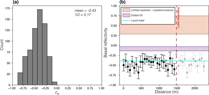
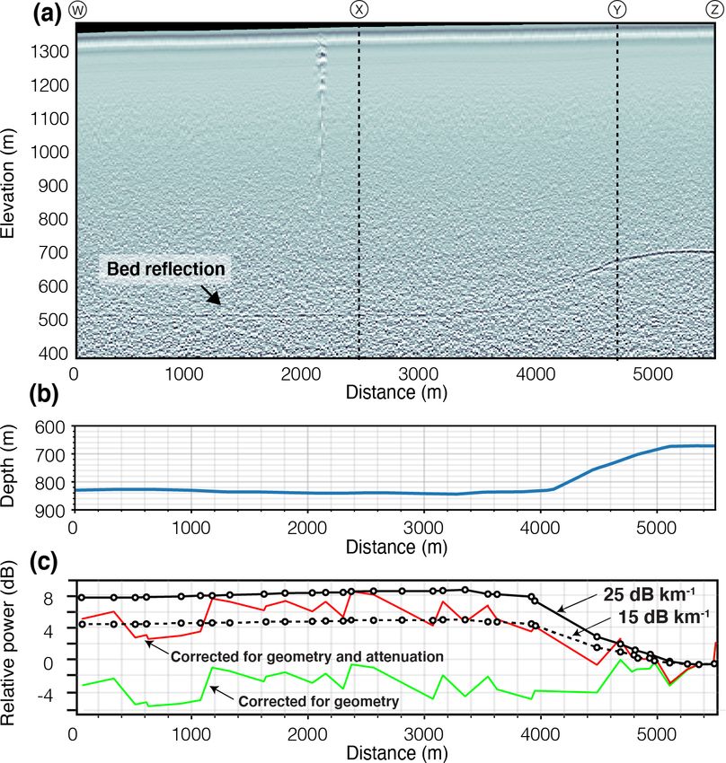
R. Maguire et al.: Geophysical constraints on the properties of a subglacial lake                                                       3283

Figure 2. (a) The seismic reflection profile of the entire traverse. Reflections labeled R1 and R2 correspond to the primary reflection from
the lake top and its multiple. A transect distance of 0 m corresponds to the southwestern end of the line. (b) A close-up of the R1 reflection
window (black rectangle in panel a), showing reflections from both the lake top and the lake bottom. Travel time picks of the lake top and
lake bottom reflections are drawn with the dashed blue line. The depth of the lake inferred from the picked reflections assuming a lake VP of
1498 m s−1 is shown in (c). Blue-shaded regions indicate where the lake bottom reflection is most clearly identified.

arriving between 14–20 ms after R1, which we interpret as                terface. However, Tulaczyk and Foley (2020) show that sub-
a lake bottom reflection (Fig. 2b). This signal is intermit-             glacial materials with high conductivity can produce similar
tently observed but is most continuous at transect distances             reflections to an ice–water interface. Additionally, Tulaczyk
between 660–1200 m. The travel time differential between                 and Foley (2020) provide a method using information about
the lake top and lake bottom reflection is used to measure               phase and multiple frequencies to better distinguish among
the thickness of the water column as a function of distance              freshwater, brine, and water- or brine-saturated clay. Our
along the transect. Assuming VP in the lake of 1498 m s−1                available data, however, are at a single frequency and do not
(Table 1), the lake is between 10–15 m deep (Fig. 2c). An                retain phase information; therefore, we do not have sufficient
uncertainty of ± 50 m s−1 in the seismic velocity of the lake            information to distinguish between these high-conductivity
would correspond to a lake depth uncertainty of ± 0.5 m. A               materials based on radar alone. The secondary seismic re-
strong coda following the lake bottom reflection is apparent,            flection discussed above suggests that the lake is water of
which is likely caused by a thin (∼ 10 m) sediment package               unknown salinity, rather than saturated sediments.
underlying the lake (see Discussion section).                               Assuming an absorption factor of a = 0.23, the average
   In the GPR profile, the subglacial lake is apparent as a flat         seismic reflection coefficient of the lake bottom across the
reflector at an elevation of ∼ 510 m along the majority of the           transect is −0.43 ± 0.17 (Fig. 4a). In Fig. 4b, we plot cR cal-
transect (Fig. 3a). The surface topography slopes gently to              culated for each shot gather above the lake as a function of
the west across the transect; hence the lake top is slightly             the distance along the transect. For comparison we show the
deeper (i.e., the ice is thicker) towards the east (Fig. 3b). The        expected reflection coefficients of several different geologic
lake is beneath 840 m of ice at transect distances between               materials underlying glacial ice. Beyond the boundary of the
2 and 4.5 km, which roughly corresponds to the location of               lake, the R2 signal strength is diminished and we are unable
the seismic survey. The transition from the lake top to the              to confidently measure cR . The reflection coefficients were
adjacent bed is observed at approximately 4100 m along the               modeled using the two-term approximation of the Zoeppritz
transect. In addition, we observe that the bed reflected power           equations (e.g., Aki and Richards, 2002; Booth et al., 2015)
is approximately 5 dB higher over the lake compared to the               with the material properties shown in Table 1. In contrast to
surrounding region (Fig. 3c). Similar to the conclusion of               other likely geological materials at the base of the ice, liquid
Palmer et al. (2013), which was based on airborne radar, we              water is expected to have a negative reflection coefficient.
infer this elevated reflectivity results from an ice–water in-           The reflection coefficient modeled for lithified sediments or

https://doi.org/10.5194/tc-15-3279-2021                                                          The Cryosphere, 15, 3279–3291, 2021
3284 R. Maguire et al.: Geophysical constraints on the properties of a subglacial lake
Figure 3. GPR profile. (a) The 5 MHz radar data, unmigrated. The primary bed reflection is marked with an arrow. Vertical dashed lines
mark the approximate endpoints of the seismic survey. The depth from the surface to the base of the ice is shown in (b). In panel (c), the
relative power of the basal reflections is shown after being corrected for geometric spreading (green line) and both geometric spreading
and depth-average attenuation of −15 dB km−1 (red line). The solid and dashed black lines show the magnitude of attenuation corrections
assuming an englacial attenuation of −25 and −15 dB km−1 , respectively.
bedrock underlying ice is similar in amplitude to liquid wa- it implies that L2 could hold a significant volume of water.
ter but opposite in sign; thus, without polarity information Assuming the imaged lake depth of approximately 15 m is
sedimentary rock strata could be mistaken for a lake sig- representative of average lake depth throughout the roughly
nature. Here, we measure R1 with an opposite polarity of 10 km2 surface area determined by radio-echo sounding, we
the source (see Fig. S4); thus, liquid water is the most likely estimate the total volume of liquid water to be 0.15 km3
explanation. However, if we are significantly overestimating (0.15 Gt of water). While this is only a small fraction of the
the magnitude of reflection coefficient due to, for example, 217 ± 32 Gt of ice that Greenland is estimated to lose each
the large uncertainties in the attenuation structure of the ice, year to glacier discharge and surface melting (Shepherd et
a layer of water-saturated dilatant till may also be able to ex- al., 2019), the net storage capacity of all of Greenland’s sub-
plain our data. glacial lakes could be appreciable.
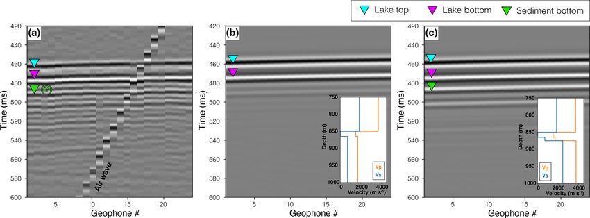
To verify our interpretation of the lake top and bottom seis-
mic reflections, we modeled synthetic seismic waveforms of
4 Discussion the 12th shot gather in our survey, which contained some
of the clearest reflections. This shot gather corresponds to
4.1 Lake geometry and volume transect distances between 660–720 m in the seismic reflec-
tion image. Synthetic seismograms were computed using
If our interpretation of the observed seismic and radar re- SPECFEM2D (Tromp et al., 2008) for two simple layered
flections as signals from the lake top and bottom is correct,
The Cryosphere, 15, 3279–3291, 2021 https://doi.org/10.5194/tc-15-3279-2021R. Maguire et al.: Geophysical constraints on the properties of a subglacial lake 3285
Figure 4. (a) Distribution of reflection coefficients cR calculated for all shots in the survey. (b) Basal reflectivity as a function of distance
along the transect. The black scatter points with error bars show the mean and standard deviation of cR in a single shot gather, calculated
assuming an absorption factor a = 0.23. The shaded regions show the range of expected basal reflectivity values for bedrock or dilatant till,
and the cyan line shows the basal reflectivity expected for liquid water. The approximate boundary of the subglacial lake is marked by the
dashed red line. Values beyond the margin of the lake are shown with light shading because they cannot be confidently interpreted due to the
low signal strength of the R2 reflection.
Table 1. Description of material properties used in reflection coefficient modeling.
Material VP (m s−1 ) VS (m s−1 ) Density (kg m−3 )
Glacial ice 3810a 1860a 920a
Water 1498a 0 1000
Dilatant sediment 1600–1800b 100–500b 1600–1800b
Lithified sediment 3000b –3750a 1200b –2450a 2200b –2450a
Bedrock 5200a –6200b 2700a –3400b 2700a –2800b
a Values are compiled from Peters et al. (2008). b Values are compiled from Christianson et
al. (2014).
models of a 12 m thick lake underlying 850 m of glacial ice. nuity at the base of the sediment package (Fig. 5b). When a
In the first model the lake is underlain by a thick layer of sed- discontinuity between the sediment and underlying bedrock
iments that extends to the bottom of the model domain. In is included, a strong sediment bottom reflection is introduced
the second model there is 10 m of sediments overlying a dis- which more closely matches the observations (Fig. 5c). In
continuity with the bedrock below. The seismic velocity pro- the observed data it is difficult to clearly identify a sediment
files for the two cases are shown in the insets in Fig. 5b and bottom reflection since the complex coda could be caused
c. The source used in the simulations was a Ricker wavelet by reverberations within a thin sediment sequence or many
with a dominant frequency of 100 Hz. Figure 5 shows a com- superposed reflections from individual discontinuities. How-
parison between the observations and synthetics. In both the ever, if the first positive peak following the lake bottom re-
observed (Fig. 5a) and synthetic (Fig. 5b and c) shot gath- flection represents the base of the sediment, we can estimate
ers, the lake top and lake bottom reflections are separated by a sediment thickness of 8.5 m assuming a sediment VP of
∼ 20 ms and show a clear polarity reversal, which reflects the 1700 m s−1 (Table 1).
opposite sign of the acoustic impedance contrast between an
ice–water and a water–lake bed transition. The observed shot 4.2 Lake origin
gather contains a coda following the lake bottom reflection
that is absent in the synthetics that do not include a disconti- While our results suggest that L2 is indeed a subglacial lake,
its presence is perplexing given its location with a mean an-
https://doi.org/10.5194/tc-15-3279-2021 The Cryosphere, 15, 3279–3291, 20213286 R. Maguire et al.: Geophysical constraints on the properties of a subglacial lake
Figure 5. Observed (a) and synthetic (b, c) seismic data for shot gather 12 bandpass filtered between 50–200 Hz. The offset from the source
to geophone 1 is 230 m. The colored triangles indicate reflections from the lake top (blue), lake bottom (purple), and sediment bottom (green).
The insets in panels (b) and (c) show the VP and VS models that were used to compute the synthetics. Both models include a 12 m thick lake
below 850 m of ice. The model used in (c) includes an additional discontinuity 10 m below the lake, which represents the boundary between
the lake bottom sediments and underlying bedrock.
nual surface temperature of −22 ◦ C and its position beneath There are several possible explanations for the existence
a relatively thin column of glacial ice. In contrast to many of liquid water underneath the ice, including hypersalinity,
well-studied subglacial lakes below the Antarctic ice sheet, recharge by surface meltwater, high geothermal flux, and la-
such as Lake Vostok, that lie below ∼ 4 km of ice, the basal tent heat from freezing. Here, we review these explanations
temperature at our field site is expected to be well below the and assess their specific relevance to lake L2.
pressure-dependent melting point of ice. Distinguishing be-
tween the different hypotheses of subglacial lake formation
has implications for the stability and dynamics of the Green- 1. Hypersalinity. If the lake is hypersaline, the lake wa-
land ice sheet since they predict different basal thermal and ter could remain liquid at low temperatures by depress-
hydrological conditions. Thus, constraining the temperature ing the freezing temperature. In order to depress the
of L2 is an important goal. freezing temperature of water by 12 to 14 ◦ C a NaCl
We determine the range of possible basal temperatures us- concentration of roughly 160 to 180 ppt would be re-
ing a 1D steady-state advection–diffusion heat transfer model quired, 6× that of seawater (e.g., Fofonoff and Mil-
solved using the control volume method (see Supplement). lard, 1983). If the hypersaline condition is restricted to
The modeling assumes an ice density of ρ = 920 kg m−3 , a the lake, the surrounding ice would likely be frozen to
heat capacity of cP = 2000 J kg−1 K−1 , and a thermal con- the bed and would form a closed hydrological system
ductivity of ice of k = 2.3 W m−1 K−1 . The basal geothermal that could remain isolated on geologic timescales. In
heat flux q is varied between 50–60 mW m−2 , which is con- this scenario, the lake could represent a body of ancient
sistent with estimates derived from magnetic data (Martos et marine water that was trapped as glacial ice advanced
al., 2018) and thermal isostasy modeling (Artemieva, 2019). over the area and was potentially further enriched in
Figure 6 shows results for surface temperatures TS of −20 salt through cryogenic concentration processes (Lyons
and −22 ◦ C and ice-equivalent accumulation rates w ranging et al., 2005, 2019). Similar hypersaline lakes with salt
from 0 to 0.3 m yr−1 . When vertical advection is ignored (i.e., concentrations several times higher than seawater are
no ice accumulation), most scenarios predict frozen bed con- known to exist below the McMurdo Dry Valleys in
ditions with the exception of the relatively warm surface con- Antarctica (Hubbard et al., 2004; Lyons et al., 2005,
dition (TS = −20 ◦ C) and high heat flow (q = 60 mW m−2 ) 2019; Mikucki et al., 2009) and in the Devon Ice Cap,
scenario (Fig. 6a). When ice accumulation is considered, all Canada (Rutishauser et al., 2018). Because the current
scenarios predict frozen bed conditions (Fig. 6b). For an elevation of the lake is more than 500 m above sea level,
ice-equivalent accumulation rate of 0.3 m yr−1 , which most it is unlikely to be trapped seawater as in the McMurdo
closely matches the conditions of the field site, and regional Dry Valleys. While an ancient evaporite deposit is pos-
average geothermal flux, the basal temperature is expected to sible, as is proposed for the Devon Ice Cap (Rutishauser
be between approximately −12 and −14 ◦ C. et al., 2018), the geologic map of Greenland does not
indicate likely evaporites in this area (Dawes, 2004).
The Cryosphere, 15, 3279–3291, 2021 https://doi.org/10.5194/tc-15-3279-2021R. Maguire et al.: Geophysical constraints on the properties of a subglacial lake 3287
cumulation area of the ice sheet, near the ice divide
(Fig. 1b), and there are no obvious sources of significant
surface recharge visible on the ground or from satel-
lite imagery. To determine possible pathways for sur-
face recharge from more distant features, we estimate
the local hydraulic head based on surface and bed ele-
vations (Fig. S5) and find no pathways given the present
resolution of the bed and surface topography. It is possi-
ble that a subglacial pathway exists that is smaller than
the resolution of BedMachine (Morlighem et al., 2017).
3. High geothermal flux. Anomalously high basal heat flux
may promote melting of the ice sheet from below (e.g.,
Fahnestock et al., 2001; Rogozhina et al., 2016). If this
is the case, the local geothermal heat flux must greatly
exceed regional estimates of the geothermal heat flux
beneath the northwestern Greenland ice sheet, which are
typically in the range of 50–60 mW m−2 (Artemieva,
2019; Martos et al., 2018; Rogozhina et al., 2016).
Based on the one-dimensional model shown in Fig. 6,
a geothermal flux on the order of 100 mW m−2 would
be necessary to sustain the lake. While high heat flux in
this region is unexpected based on the cratonic bedrock
geology and lack of recent volcanism, a local region of
high heat flux could be promoted by the presence of up-
per crustal granitoids rich in radiogenic heat-producing
elements or hydrothermal fluid migration through pre-
existing fault systems (e.g., Jordan et al., 2018).
4. Latent heat from freezing. For the isolated lake of ac-
tively freezing brine (as in Hypothesis 1), the hydrolog-
ically connected continuous flow (Hypothesis 2), or if
the lake is a relic of a larger freshwater body that is
slowly freezing, the thermal profile of the ice would
show a curvature change at depth due to a latent heat
source at the bottom boundary. Given a latent heat of
freezing of 334 J g−1 , freezing a layer 1 m thick to the
Figure 6. Modeled ice-sheet thermal structure. Panel (a) shows
bottom of the ice over 1 year is roughly equivalent to
thermal profiles neglecting advection for surface temperatures of
TS = −22 ◦ C and TS = −20 ◦ C. Panel (b) shows thermal pro- increasing the geothermal flux by 10 mW m−2 .
files including advection for a fixed surface temperature of TS =
Sustaining a freezing rate of several m yr−1 to generate the
−22 ◦ C. The basal heat flux q is varied between 50–60 mW m−2 ,
latent heat necessary to maintain warm basal ice is less likely
and the accumulation rate w is varied between 0 and 0.3 m yr−1 .
than a locally elevated geothermal anomaly. We, therefore,
narrow the lake origin hypotheses to either anomalously high
geothermal flux or hypersalinity due to local ancient evapor-
2. Surface meltwater. The lake may be part of an open hy- ite. Measuring the thermal profile and vertical velocity and
drological system that is continually recharged by sur- strain rates above this lake would provide important informa-
face meltwater. If the hydrological system is connected tion to assess these hypotheses. For a freshwater lake created
and the rate of recharge matches or exceeds the rate of by high geothermal flux, the basal ice temperature would be
freezing, a lake could persist despite sub-freezing tem- near 0 ◦ C, and vertical velocity would be downward if melt-
peratures in the lower part of the ice. At other locations ing exceeds accumulation. For a lake created by evaporite,
in Greenland, observations of vertical surface deforma- the basal ice would be substantially below zero, and the ver-
tion and collapse features have suggested that surface tical velocity would be near zero or upward (due to freez-
meltwater plays a prominent role in subglacial lake for- ing). A geothermally created lake would show higher verti-
mation and dynamics (Palmer et al., 2015; Willis et al., cal strain rates in the lower part of the ice column than an
2015). This lake, however, is in the high-elevation ac- evaporite-created lake.
https://doi.org/10.5194/tc-15-3279-2021 The Cryosphere, 15, 3279–3291, 20213288 R. Maguire et al.: Geophysical constraints on the properties of a subglacial lake
A freshwater lake and a hypersaline lake have different constraints on its depth. Understanding the nature and ori-
physical properties and thus may have different signatures gins of recently detected subglacial lakes in Greenland is im-
that could be detected in geophysical surveys. Radar reflec- portant since wet basal conditions enable glacial ice to flow
tions from an ice–brine boundary undergoing freezing and more easily which can further promote ice loss. Our analysis
cryoconcentration of the brine are known to cause scattering of the seismic and radar, as well as thermal and hydropo-
and decrease the reflectivity (Badgeley et al., 2017), which tential, analysis narrow the lake origins to either locally high
we do not see in our data; this provides a second justification geothermal flux or an ancient evaporite deposit. Future work,
to rule out modern active cryoconcentration; in addition, sus- such as additional geophysical investigations or drilling ex-
tained freezing of any ice is likely to create a radar-detectable peditions, should focus on constraining the temperature and
basal ice unit such as that suggested by Bell et al. (2014). salinity of the lake which will provide clues to its origin.
Further, because the seismic velocity and density of water
depends on temperature and salinity, we would expect that
lakes formed by different mechanisms would have slightly Code availability. All seismic processing performed in this study
different basal reflection coefficients, although the small vari- was performed using ObsPy (Beyreuther et al., 2010), which is an
ations expected in cR would not be resolvable with our data openly available Python-based software package.
set. On the other hand, because the electrical resistivity of
water is strongly dependent on salinity, magnetic sounding
could provide useful constraints on lake composition. Addi- Data availability. Active-source seismic data, including a full de-
scription of the data set, are available through the Digital Repository
tionally, since radar attenuation is strongly sensitive to lake
at the University of Maryland (https://doi.org/10.13016/yy2o-nhua,
conductivity, radio-echo sounding amplitude data could po-
Schmerr et al., 2021). GPR data are available on request from the
tentially help constrain salinity if lake bed returns are ob- corresponding author.
served in shallow areas. Stronger constraints could poten-
tially be placed on subglacial properties if a stronger active-
source were used (e.g., explosives), since data with a high Supplement. The supplement related to this article is available on-
signal-to-noise ratio could be recorded at larger distances. line at: https://doi.org/10.5194/tc-15-3279-2021-supplement.
This would be particularly useful for measuring the basal re-
flectivity as a function of the incidence angle, which would
help verify our interpretation of a subglacial lake. Repeated Author contributions. This project was conceptualized by the SI-
seismic reflection or GPR surveys calculated along the same IOS (Seismometer to Investigate Ice and Ocean Structure) team.
transect could provide clues to whether or not lake levels are Analysis of the seismic data was performed by RM and CG with
changing over time (e.g., Church et al., 2020). Finally, direct support from NS and KR. EP performed the GPR analysis and ther-
sampling with drilling would provide the best measurements mal modeling. RM was the lead on manuscript writing and figure
on subglacial lake properties and could also yield useful bio- preparation, with significant inputs from EP, NS, and KR. Authors
DND, NW, BA, AGM, NH were essential for data collection and
logical and paleoenvironmental information.
curation. JIB, VJB, and SHB were project administrators and also
provided critical review and commentary.
5 Conclusions
Competing interests. The authors declare that they have no conflict
We conducted an active-source seismic reflection and GPR of interest.
survey in northwestern Greenland above a site that was pre-
viously identified as a possible subglacial lake. We observed
a horizontal reflector across the majority survey with a seis- Disclaimer. Publisher’s note: Copernicus Publications remains
mic reflection coefficient of −0.43 ± 0.17, consistent with neutral with regard to jurisdictional claims in published maps and
the presence of a lake below approximately 830–845 m of institutional affiliations.
ice. Additionally, we observed a lake bottom reflection near
the center of our seismic profile consistent with a lake depth
of approximately 15 m. From previous observations of the Acknowledgements. The authors thank SIIOS (Seismometer to In-
lateral extent of the lake based on airborne radio-echo sound- vestigate Ice and Ocean Structure) team members Chris Carr and
ing (Palmer et al., 2013), we estimate the subglacial lake Renee Weber for helpful discussions. Additionally, we thank the
holds a total of 0.15 Gt of water. A strong coda arriving af- editor Evgeny A. Podolskiy, the two anonymous reviewers, and Ja-
cob Buffo for feedback that helped improve this study. Logistical
ter the lake-bottom reflection suggests that the lake is under-
support for fieldwork in northwestern Greenland was provided by
lain by a sedimentary package, but its thickness and material Susan Detweiler.
properties are uncertain. To the authors knowledge, this is the
first time a ground-based geophysical survey has confirmed
the existence of a subglacial lake in Greenland and provided
The Cryosphere, 15, 3279–3291, 2021 https://doi.org/10.5194/tc-15-3279-2021R. Maguire et al.: Geophysical constraints on the properties of a subglacial lake 3289
Financial support. Funding for this work was provided by the Commun., 10, 1–11, https://doi.org/10.1038/s41467-019-10821-
NASA Planetary Science and Technology Through Analog Re- w, 2019.
search (PSTAR) (grant no. 80NSSC17K0229). Additionally, Campen, R., Kowalski, J., Lyons, W. B., Tulaczyk, S., Dachwald,
Nicholas Schmerr received support from the NASA Solar Sys- B., Pettit, E., Welch, K. A., and Mikucki, J. A.: Micro-
tem Exploration Research Virtual Institute (SSERVI) Geophysical bial diversity of an Antarctic subglacial community and high-
Exploration of the Dynamics and Evolution of the Solar System resolution replicate sampling inform hydrological connectiv-
(GEODES) (grant no. 80NSSC19M0216). ity in a polar desert, Environ. Microbiol., 21, 2290–2306,
https://doi.org/10.1111/1462-2920.14607, 2019.
Christianson, K., Peters, L. E., Alley, R. B., Anandakrish-
Review statement. This paper was edited by Evgeny A. Podolskiy nan, S., Jacobel, R. W., Riverman, K. L., Muto, A., and
and reviewed by two anonymous referees. Keisling, B. A.: Dilatant till facilitates ice-stream flow in
northeast Greenland, Earth Planet. Sc. Lett., 401, 57–69,
https://doi.org/10.1016/j.epsl.2014.05.060, 2014.
Christianson, K., Jacobel, R. W., Horgan, H. J., Alley, R. B.,
References Anandakrishnan, S., Holland, D. M., and DallaSanta, K. J.:
Basal conditions at the grounding zone of Whillans Ice Stream,
Achberger, A. M., Christner, B. C., Michaud, A. B., Priscu, West Antarctica, from ice-penetrating radar, J. Geophys. Res.-
J. C., Skidmore, M. L., Vick-Majors, T. J., Adkins, W., Earth, 121, 1954–1983, https://doi.org/10.1002/2015JF003806,
Anandakrishnan, S., Barbante, C., Barcheck, G., and 2016.
Beem, L.: Microbial community structure of subglacial Church, G., Grab, M., Schmelzbach, C., Bauder, A., and Mau-
lake Whillans, West Antarctica, Front. Microbiol., 7, 1457, rer, H.: Monitoring the seasonal changes of an englacial conduit
https://doi.org/10.3389/fmicb.2016.01457, 2016. network using repeated ground-penetrating radar measurements,
Aki, K. and Richards, P. G.: Quantitative Seismology, University The Cryosphere, 14, 3269–3286, https://doi.org/10.5194/tc-14-
Science Books, Sausalito, CA, 2nd edn., 123–144, 2002. 3269-2020, 2020.
Artemieva, I. M.: Lithosphere thermal thickness and Dasgupta, R. and Clark, R.A.: Estimation of Q from sur-
geothermal heat flux in Greenland from a new ther- face seismic reflection data, Geophysics, 63, 2120–2128,
mal isostasy method, Earth-Sci. Rev., 188, 469–481, https://doi.org/10.1190/1.1444505, 1998.
https://doi.org/10.1016/j.earscirev.2018.10.015, 2019. Dawes, P. R.: Explanatory notes to the geological map of Green-
Badgeley, J. A., Pettit, E. C., Carr, C. G., Tulaczyk, S., land, 1 : 500 000, Humboldt Gletscher, Sheet 6, Geological
Mikucki, J. A., and Lyons, W. B.: An englacial hydro- Survey of Denmark and Greenland Map Series, 1, 1–48,
logic system of brine within a cold glacier: Blood Falls, https://doi.org/10.34194/geusm.v1.4615, 2004.
McMurdo Dry Valleys, Antarctica, J. Glaciol., 63, 387–400, Dee, D. P., Uppala, S. M., Simmons, A. J., Berrisford, P., Poli,
https://doi.org/10.1017/jog.2017.16, 2017. P., Kobayashi, S., Andrae, U., Balmaseda, M. A., Balsamo, G.,
Bell, R. E., Studinger, M., Shuman, C. A., Fahnestock, M. A., Bauer, P., Bechtold, P., Beljaars, A. C. M., van de Berg, L., Bid-
and Joughin, I.: Large subglacial lakes in East Antarctica at lot, J., Bormann, N., Delsol, C., Dragani, R., Fuentes, M., Geer,
the onset of fast-flowing ice streams, Nature, 445, 904–907, A. J., Haimberger, L., Healy, S. B., Hersbach, H., Hólm, E. V.,
https://doi.org/10.1038/nature05554, 2007. Isaksen, L., Kållberg, P., Köhler, M., Matricardi, M., McNally,
Bell, R. E., Tinto, K., Das, I., Wolovick, M., Chu, W., Creyts, T. T., A. P., Monge-Sanz, B. M., Morcrette, J. J., Park, B. K., Peubey,
Frearson, N., Abdi, A., and Paden, J. D.: Deformation, warming C., de Rosnay, P., Tavolato, C., Thépaut, J. N., and Vitart, F.: The
and softening of Greenland’s ice by refreezing meltwater, Nat. ERA-Interim reanalysis: configuration and performance of the
Geosci., 7, 497–502, https://doi.org/10.1038/ngeo2179, 2014. data assimilation system, Q. J. Roy. Meteor. Soc., 137, 553–597,
Bentley, C. R. and Kohnen, H.: Seismic refraction measurements https://doi.org/10.1002/qj.828, 2011.
of internal friction in Antarctic ice, J. Geophys. Res., 81, 1519– Fahnestock, M., Abdalati, W., Joughin, I., Brozena, J., and Gogi-
1526, https://doi.org/10.1029/JB081i008p01519, 1976. neni, P.: High geothermal heat flow, basal melt, and the origin
Bentley, M. J., Christoffersen, P., Hodgson, D. A., Smith, A. M., of rapid ice flow in central Greenland, Science, 294, 2338–2342,
Tulaczyk, S., and Le Brocq, A. M.: Subglacial lake sediments https://doi.org/10.1126/science.1065370, 2001.
and sedimentary processes: potential archives of ice sheet evo- Filina, I. Y., Blankenship, D. D., Thoma, M., Lukin, V. V.,
lution, past environmental change, and the presence of life, in: Masolov, V. N., and Sen, M. K.: New 3D bathymetry and
Antarctic Subglacial Aquatic Environments, American Geophys- sediment distribution in Lake Vostok: Implication for pre-
ical Union, Washington, D.C., 83–110, 2011. glacial origin and numerical modeling of the internal pro-
Beyreuther, M., Barsch, R., Krischer, L., Megies, T., cesses within the lake, Earth Planet. Sc. Lett., 276, 106–114,
Behr, Y., and Wassermann, J.: ObsPy: A Python tool- https://doi.org/10.1016/j.epsl.2008.09.012, 2008.
box for seismology, Seismol. Res. Lett., 81, 530–533, Fofonoff, N. P. and Millard Jr., R. C.: Algorithms for computation
https://doi.org/10.1785/gssrl.81.3.530, 2010. of fundamental properties of seawater, Unesco Tech. Pap. Mar.
Booth, A. D., Emir, E., and Diez, A.: Approximations to seismic Sci., 44, 1–58, 1983.
AVA responses: Validity and potential in glaciological appli- Fricker, H. A., Scambos, T., Bindschadler, R., and Pad-
cations, Geophysics, 81, 1–11, https://doi.org/10.1190/geo2015- man, L.: An Active Subglacial Water System in West
0187.1, 2016. Antarctica Mapped from Space, Science, 315, 1544–1548,
Bowling, J. S., Livingstone, S. J., Sole, A. J., and Chu, W.: https://doi.org/10.1126/science.1136897, 2007.
Distribution and dynamics of Greenland subglacial lakes, Nat.
https://doi.org/10.5194/tc-15-3279-2021 The Cryosphere, 15, 3279–3291, 20213290 R. Maguire et al.: Geophysical constraints on the properties of a subglacial lake Hills, B. H., Christianson, K., and Holschuh, N.: A framework power, central West Antarctica, J. Geophys. Res., 115, 1–15, for attenuation method selection evaluated with ice-penetrating https://doi.org/10.1029/2009JF001496, 2010. radar data at south pole lake, Ann. Glaciol., 61, 176–187, Mikucki, J. A., Pearson, A., Johnston, D. T., Turchyn, A. https://doi.org/10.1017/aog.2020.32, 2020. V., Farquhar, J., Schrag, D. P., Anbar, A. D., Priscu, J. Horgan, H. J., Anandakrishnan, S., Jacobel, R. W., Christianson, C., and Lee, P. A.: A contemporary microbially main- K., Alley, R. B., Heeszel, D. S., Picotti, S., and Walter, J. I.: Sub- tained subglacial ferrous “Ocean”, Science, 324, 397–400, glacial Lake Whillans-Seismic observations of a shallow active https://doi.org/10.1126/science.1167350, 2009. reservoir beneath a West Antarctic ice stream, Earth Planet. Sc. Morlighem, M., Williams, C. N., Rignot, E., An, L., Arndt, J. E., Lett., 331, 201–209, https://doi.org/10.1016/j.epsl.2012.02.023, Bamber, J. L., Catania, G., Chauche, N., Dowdeswell, J. A., 2012. Dorschel, B., Fenty, I., Hogan, K., Howat, I., Hubbard, A., Jakob- Hubbard, A., Lawson, W., Anderson, B., Hubbard, B., and sson, M., Jordan, T. M., Kjeldsen, K. K., Millan, R., Mayer, L., Blatter, H.: Evidence for subglacial ponding across Taylor Mouginot, J., Noel, B. P. Y., O’Cofaigh, C., Palmer, S., Rys- Glacier, Dry Valleys, Antarctica, Ann. Glaciol., 39, 79–84, gaard, S., Seroussi, H., Siegert, M. J., Slabon, P., Straneo, F., van https://doi.org/10.3189/172756404781813970, 2004. den Broeke, M. R., Weinrebe, W., Wood, M., and Zinglersen, Jacobel, R. W., Welch, B. C., Osterhouse, D., Pettersson, R., and K. B.: BedMachine v3: Complete Bed Topography and Ocean Gregor, J. A. M.: Spatial variation of radar-derived basal condi- Bathymetry Mapping of Greenland From Multibeam Echo tions on Kamb Ice Stream, West Antarctica, Ann. Glaciol., 50, Sounding Combined With Mass Conservation, Geophys. Res. 10–16, https://doi.org/10.3189/172756409789097504, 2009. Lett., 44, 11051–11061, https://doi.org/10.1002/2017GL074954, Jordan, T., Martin, C., Ferraccioli, F., Matsuoka, K., Corr, H., 2017. Forsberg, R., Olesen, A., and Siegert, M.: Anomalously high Noël, B., van de Berg, W. J., van Wessem, J. M., van Meij- geothermal flux near the South Pole, Sci. Rep.-UK, 8, 16785, gaard, E., van As, D., Lenaerts, J. T. M., Lhermitte, S., Kuipers https://doi.org/10.1038/s41598-018-35182-0, 2018. Munneke, P., Smeets, C. J. P. P., van Ulft, L. H., van de Wal, Jordan, T. M., Cooper, M. A., Schroeder, D. M., Williams, C. N., R. S. W., and van den Broeke, M. R.: Modelling the climate Paden, J. D., Siegert, M. J., and Bamber, J. L.: Self-affine sub- and surface mass balance of polar ice sheets using RACMO2 – glacial roughness: consequences for radar scattering and basal Part 1: Greenland (1958–2016), The Cryosphere, 12, 811–831, water discrimination in northern Greenland, The Cryosphere, 11, https://doi.org/10.5194/tc-12-811-2018, 2018. 1247–1264, https://doi.org/10.5194/tc-11-1247-2017, 2017. Palmer, S. J., Dowdeswell, J. A., Christoffersen, P., Young, Langley, K., Kohler, J., Matsuoka, K., Sinisalo, T., Scam- D. A., Blankenship, D. D., Greenbaum, J. S., Benham, bos, T., Neumann, T., Muto, A., Winther, J.-G., and Albert, T., Bamber, J., and Siegert, M. J.: Greenland subglacial M.: Recovery Lakes, East Antarctica: Radar assessment of lakes detected by radar, Geophys. Res. Lett., 40, 6154–6159, sub-glacial water extent, Geophys. Res. Lett., 38, L05501, https://doi.org/10.1002/2013GL058383, 2013. https://doi.org/10.1029/2010GL046094, 2011. Palmer, S., McMillan, M., and Morlighem, M.: Subglacial lake Lyons, W. B., Welch, K. A., Snyder, G., Olesik, J., Graham, E. Y., drainage detected beneath the Greenland ice sheet, Nat. Com- Marion, G. M., and Poreda, R. J.: Halogen geochemistry of the mun., 6, 8408, https://doi.org/10.1038/ncomms9408, 2015. McMurdo Dry Valleys lakes, Antarctica: clues to the origin of Peters, L. E., Anandakrishnan, S., Holland, C. W., Horgan, H. J., solutes and lake evolution, Geochim. Cosmochim. Ac., 69, 305– Blankenship, D. D., and Voigt, D. E.: Seismic detection of a sub- 323, https://doi.org/10.1016/j.gca.2004.06.040, 2005. glacial lake near the South Pole, Antarctica, Geophys. Res. Lett., Lyons, W. B., Mikucki, J. A., German, L. A., Welch, K. A., Welch, 35, L23501, https://doi.org/10.1029/2008GL035704, 2008. S. A., Gardner, C. B., Tulaczyk, S. M., Pettit, E. C., Kowalski, Peters, L. E., Anandakrishnan, S., Alley, R. B., and Voigt, J., and Dachwald, B.: The geochemistry of englacial brine from D. E.: Seismic attenuation in glacial ice: A proxy for Taylor Glacier, Antarctica, J. Geophys. Res.-Biogeo., 124, 633– englacial temperature, J. Geophys. Res.-Earth, 117, F02008, 648, https://doi.org/10.1029/2018JG004411, 2019. https://doi.org/10.1029/2011JF002201, 2012. MacGregor, J., Li, J., Paden, J., Catania, G., Clow, G., Fahne- Robin, G. de Q., Swithinbank, C., and Smith, B. M. E.: Radio echo stock, M., Gogineni, S., Grimm, R., Morlighem, M., Nandi, S., exploration of the Antarctic ice sheet, in: International Sympo- Seroussi, H., and Stillman, D.: Radar attenuation and tempera- sium on Antarctic Glaciological Exploration (ISAGE), edited by: ture within the Greenland Ice Sheet, J. Geophys. Res.-Sol. Ea., Gow, A. J., Keeler, C., Langway, C. C., Weeks, W. F., Interna- 120, 983–1008, https://doi.org/10.1002/2014JF003418, 2015. tional Association of Scientific Hydrology, Hanover, New Hamp- MacGregor, J. A., Fahnestock, M. A., Catania, G. A., As- shire, 3–7 September 1968, Gentbrugge, IASH Publication, 86, chwanden, A., Clow, G. D., Colgan, W. T., Gogineni, S. P., 97–115, 1970. Morlighem, M., Nowicki, S. M. J., Paden, J. D., Price, S. F., Rogozhina, I., Petrunin, A. G., Vaughan, A. P. M., Steinberger, B., and Seroussi, H.: A synthesis of the basal thermal state of the Johnson, J. V., Kaban, M. K., Calov, R., Rickers, F., Thomas, M., Greenland Ice Sheet, J. Geophys. Res.-Earth, 121, 1328–1350, and Koulakov, I.: Melting at the base of the Greenland ice sheet https://doi.org/10.1002/2015JF003803, 2016. explained by Iceland hotspot history, Nat. Geosci., 9, 366–369, Martos, Y. M., Jordan, T. A., Catalan, M., Jordan, T. M., Bamber, https://doi.org/10.1038/ngeo2689, 2016. J. L., and Vaughan, D. G.: Geothermal heat flux reveals the Ice- Rutishauser, A., Blankenship, D. D., Sharp, M., Skidmore, M. L., land hotspot track underneath Greenland, Geophys. Res. Lett., Greenbaum, J. S., Grima, C., Schroeder, D. M., Dowdeswell, J. 45, 8214–8222, https://doi.org/10.1029/2018GL078289, 2018. A., and Young, D. A.: Discovery of a hypersaline subglacial lake Matsuoka, K., Morse, D., and Raymond, C. F.: Estimating complex beneath Devon Ice Cap, Canadian Arctic, Sci. Adv., 4, englacial radar attenuation using depth profiles of the returned eaar4353, https://doi.org/10.1126/sciadv.aar4353, 2018. The Cryosphere, 15, 3279–3291, 2021 https://doi.org/10.5194/tc-15-3279-2021
R. Maguire et al.: Geophysical constraints on the properties of a subglacial lake                                                       3291

Schmerr, N., Maguire, R., Pettit, E., Riverman, K., Gardner, C., Del-    Smith, B. E., Fricker, H. A., Joughin, I. R., and Tulaczyk,
   laGiustina, D., Avenson, B., Wagner, N., Marusiak, A., Habib,            S.: An inventory of active subglacial lakes in Antarctica
   N., Broadbeck, J., Bray, V., Bailey, S., Carr, C., Dahl, P., and         detected by ICESat (2003–2008), J. Glaciol., 55, 573–595,
   Weber, R.: Northwest Greenland Active Source Seismic Experi-             https://doi.org/10.3189/002214309789470879, 2009.
   ment [data set], Digital Repository at the University of Maryland,    Stearns, L. A., Smith, B. E., and Hamilton, G. S.: In-
   https://doi.org/10.13016/yy2o-nhua, 2021.                                creased flow speed on a large East Antarctic outlet
Shepherd, A., Ivins, E., Rignot, E., Smith, B., van den Broeke, M.,         glacier caused by subglacial floods, Nat. Geosci., 1, 827,
   Velicogna, I., Whitehouse, P., Briggs, K., Joughin, I., Krinner,         https://doi.org/10.1038/ngeo356, 2008.
   G., Nowicki, S., Payne, T., Scambos, T., Schlegel, N., Geruo, A.,     Tromp, J., Komatitsch, D., and Liu, Q.: Spectral-element and ad-
   Agosta, C., Ahlstrøm, A., Babonis, G., Barletta, V., Bjørk A.,           joint methods in seismology, Commun. Comput. Phys., 3, 1–32,
   Blazquez, A., Bonin, J., Colgan, W., Csatho, B., Cullather, R.,          2008.
   Engdahl, M. E., Felikson, D., Fettweis, X., Forsberg, R., Hogg,       Tulaczyk, S. M. and Foley, N. T.: The role of electrical conductivity
   A., Gallee, H., Gardner, A., Gilbert, L., Gourmelen, N., Groh,           in radar wave reflection from glacier beds, The Cryosphere, 14,
   A., Gunter, B., Hanna, E., Harig, C., Helm, V., Horvath, A., Hor-        4495–4506, https://doi.org/10.5194/tc-14-4495-2020, 2020.
   wath, M., Khan, S., Kjeldsen, K. K., Konrad, H., Langen, P.,          Vick-Majors, T. J., Mitchell, A. C., Achberger, A. M., Christner, B.
   Lecavalier, B., Loomis, B., Luthcke, S., McMillan, M., Melini,           C., Dore, J. E., Michaud, A. B., Mikucki, J. A., Purcell, A. M.,
   D., Mernild, S., Mohajerani, Y., Moore, P., Mottram, R., Moug-           Skidmore, M. L., and Priscu, J. C.: Physiological ecology of mi-
   inot, J., Moyano, G., Muir, A., Nagler, T., Nield, G., Nilsson, J.,      croorganisms in subglacial Lake Whillans, Front. Microbiol., 7,
   Noël, B., Otosaka, I., Pattle, M. E., Peltier, W. R., Pie, N., Ri-       1705, https://doi.org/10.3389/fmicb.2016.01705, 2016.
   etbroek, R., Rott, H., Sandberg-Sørensen, L., Sasgen, I., Save,       Welch, B. C. and Jacobel, R. W.: Analysis of deep-penetrating radar
   H., Scheuchl, B., Schrama, E., Schröder, L., Seo, K.-W., Simon-          surveys of West Antarctica, US-ITASE 2001, Geophys. Res.
   sen, S., Slater, T., Spada, G., Sutterley, T., Talpe, M., Tarasov,       Lett., 30, 1444, https://doi.org/10.1029/2003GL017210, 2003.
   L., van de Berg, W. J., van der Wal, W., van Wessem, M., Vish-        Willis, M., Herried, B., Bevis, M., and Bell, R.: Recharge of a sub-
   wakarma, B. D., Wiese, D., Wilton, D., Wagner, T., Wouters, B.,          glacial lake by surface meltwater in northeast Greenland, Nature,
   and Wuite, J.: Mass balance of the Antarctic Ice Sheet from 1992         518, 223–227, https://doi.org/10.1038/nature14116, 2015.
   to 2018, Nature, 558, 219–222, https://doi.org/10.1038/s41586-        Woodward, J., Smith, A. M., Ross, N., Thoma, M., Corr, H., King,
   019-1855-2, 2018.                                                        E. C., King, M., Grosfeld, K., Tranter, M., and Siegert, M.: Lo-
Siegert, M., Dowdeswell, J., Gorman, M., and McIntyre, N.: An in-           cation for direct access to subglacial Lake Ellsworth: An assess-
   ventory of Antarctic sub-glacial lakes, Antarc. Sci., 8, 281–286,        ment of geophysical data and modeling, Geophys. Res. Lett., 37,
   https://doi.org/10.1017/S0954102096000405, 1996.                         L11501, https://doi.org/10.1029/2010GL042884, 2010.
Siegfried, M. R. and Fricker, H. A.: Thirteen years of subglacial lake   Wright, A. and Siegert, M.: A fourth inventory of
   activity in Antarctica from multi-mission satellite altimetry, Ann.      Antarctic subglacial lakes, Antarct. Sci., 24, 659–664,
   Glaciol., 59, 42–55, https://doi.org/10.1017/aog.2017.36, 2018.          https://doi.org/10.1017/S095410201200048X, 2012.
Siegfried, M. R., Fricker, H. A., Carter, S. P., and Tulaczyk,           Young, D. A., Schroeder, D. M., Blankenship, D. D., Kempf, S. D.,
   S.: Episodic ice velocity fluctuations triggered by a subglacial         and Quartini, E.: The distribution of basal water between Antarc-
   flood in West Antarctica, Geophys. Res. Lett., 43, 2640–2648,            tic subglacial lakes from radar sounding, Philos. T. Roy. Soc. A.,
   https://doi.org/10.1002/2016GL067758, 2016.                              374, 20140297, https://doi.org/10.1098/rsta.2014.0297, 2016.
Smith, A. M., Woodward, J., Ross, N., Bentley, M. J., Hodg-
   son, D. A., Siegert, M. J., and King, E. C.: Evidence
   for the long-term sedimentary environment in an Antarc-
   tic subglacial lake, Earth Planet. Sci. Lett., 504, 139–151,
   https://doi.org/10.1016/j.epsl.2018.10.011, 2018.

https://doi.org/10.5194/tc-15-3279-2021                                                         The Cryosphere, 15, 3279–3291, 2021
You can also read