An information theoretic approach to link prediction in multiplex networks - Nature
←
→
Page content transcription
If your browser does not render page correctly, please read the page content below
www.nature.com/scientificreports
OPEN An information theoretic approach
to link prediction in multiplex
networks
Seyed Hossein Jafari*, Amir Mahdi Abdolhosseini‑Qomi, Masoud Asadpour,
Maseud Rahgozar & Naser Yazdani
The entities of real-world networks are connected via different types of connections (i.e., layers).
The task of link prediction in multiplex networks is about finding missing connections based on both
intra-layer and inter-layer correlations. Our observations confirm that in a wide range of real-world
multiplex networks, from social to biological and technological, a positive correlation exists between
connection probability in one layer and similarity in other layers. Accordingly, a similarity-based
automatic general-purpose multiplex link prediction method—SimBins—is devised that quantifies
the amount of connection uncertainty based on observed inter-layer correlations in a multiplex
network. Moreover, SimBins enhances the prediction quality in the target layer by incorporating the
effect of link overlap across layers. Applying SimBins to various datasets from diverse domains, our
findings indicate that SimBins outperforms the compared methods (both baseline and state-of-the-art
methods) in most instances when predicting links. Furthermore, it is discussed that SimBins imposes
minor computational overhead to the base similarity measures making it a potentially fast method,
suitable for large-scale multiplex networks.
Link prediction has been an area of interest in the research of complex networks for over two decades1, studying
the relationships between entities (nodes) in data represented as graphs. The main goal is to reveal the underlying
truth behind emerging or missing connections between node pairs of a network. Link prediction methods have
a wide range of applications, from discovery of latent and spurious interactions in biological networks (which
is basically quite costly if performed in traditional methods)2,3 to recommender s ystems4,5 and better routing in
wireless mobile n etworks6. Numerous perspectives have been adopted to attack the problem of link prediction.
According to similarity-based methods, similarity between nodes determines their likelihood of linkage. This
approach is a result of assuming that two nodes are similar if they share many common f eatures7. A whole lot of
nodes’ features stay hidden (or are kept hidden intentionally) in real networks. Further, an interesting question
is, despite the fact that a considerable amount of information is hidden in a network, what fraction of the truth
can still be extracted by merely including structural features? That is one of the main drives to utilize structural
similarity indices for link prediction. Several different classifications of similarity measures have been proposed,
among all, classifying based on locality of indices is of great importance. To name a few, Common Neighbors
(CN)1, Preferential Attachment (PA)8, Adamic-Adar (AA)9 and Resource Allocation (RA)10 are popular indices
focusing mostly on nodes’ structural features, each with unique characteristics. Even though these indexes are
simple, they are popular because of their low computational cost and reasonable prediction performance. On
the other hand, global indices take features of the whole network structure into account, tolerating higher cost
of computation, usually in favor of more accurate information. Take length of paths between pairs of nodes for
instance, which the well-known K atz11 index operates on. Average Commute Time (ACT)1 and PageRank12 are
some other notable global indices. In between lie the quasi-local methods which are able to combine properties
from both local and global indices, meaning they include global information, but their computational complexity
is similar to that of local methods, such as the Local Path (LP)13 index and Local Random Walk (LRW)14. For
more detailed information on these similarity indices (also described as unsupervised methods in the l iterature15),
readers are advised to refer t o16.
Some researchers have tackled the link prediction problem using the ideas of information theory. These works
are based on the fact that similarity of node pairs can be written in term of the uncertainty of their connectivity.
At the beginning, the uncertainty of connectivity can be estimated based on priors. Later, all structures around
the unconnected node pairs can be considered as evidences to reduce the level of uncertainty in connectedness
School of Electrical and Computer Engineering, College of Engineering, University of Tehran, Tehran, Iran. *email:
jafari.h@ut.ac.ir
Scientific Reports | (2021) 11:13242 | https://doi.org/10.1038/s41598-021-92427-1 1
Vol.:(0123456789)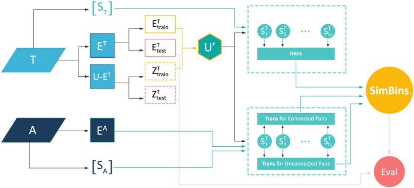
www.nature.com/scientificreports/
of node pairs. I n17 mutual information (MI) of common neighbors is incorporated to estimate the connection
likelihood of a node pair. In addition, Path Entropy (PE)18 similarity index takes quantity and length of paths as
well as theirentropy into account. This results in a better assessment of connection likelihood for node pairs. In19,
authors proposed an information theoretic method to benefit from several structural features at the same time.
By using information theory, they score each structural feature separately and then combine them by weighted
summation. Then they apply the idea on common neighbors and connectivity of neighbor sets as two structural
features. Although, most of literature about link prediction is devoted to unweighted networks but a few works
have targeted the weighted networks. In20, authors use a weighted mutual information to predict weighted links
which benefits from both structural properties and link weights. The results are promising when compared to
both weighted and unweighted methods.
In a coarse-grained sense, learning-based link prediction models reside in a different class than aforemen-
tioned similarity-based ones. They learn a group of parameters by processing input graph and use certain models,
such as feature-based prediction ( HPLP21) and latent feature extraction (Matrix F actorization15). Representation
learning has helped automating the entire process of link prediction, especially feature selection; node2vec22 and
DGI23, for instance. Recently, an interesting multiplex embedding model has also been proposed called D MGI24
which is basically an extension of DGI. Learning-based methods often yield better results than their similarity-
based counterparts, but that does not mean these models are obsolete. On the one hand, similarity-based models
provide a better understanding of the underlying characteristics of networks. Take common neighbors (CN) for
example, which indicates the high clustering property of networks18 or Adamic-Adar index which is based on the
size of common nodes’ n eighborhoods9. On the other hand, similarity-based methods often take less computation
effort, making them suitable for online prediction without costly training procedures or feature selection stages25.
Related works
Complex networks research was focused on single-layer networks (simplex or mono-plex) for many years. The
study of multi-layer (multiplex or heterogeneous) networks has gained the attention of researchers in the past
few years. Refs.26,27 provide noteworthy reviews on history of multi-layer networks. The attempts to predict
multi-layer links are not abundant and some are discussed here.
Hidden geometric correlation in real multiplex n etworks28 is an interesting work which depicts how multiplex
networks are not just random combinations of single-layer networks. They employ these geometric correlations
for trans-layer link prediction i.e., incorporating observations of other layers for predicting connections in a
specific layer. This work is followed by a study that argues the requirement of a link persistence factor to explain
high edge overlap in real multiplex systems29. In heterogeneous networks (i.e., networks with different types
of nodes and relations), several similarity-search approaches have been proposed. PathSim30 is a meta path-
based similarity measure that can find similar peers in heterogeneous networks (e.g. authors in similar fields
in a bibliographic network). The intuition behind PathSim is that two peer objects are similar if they are not
only strongly connected, but also share comparable visibility (number of path instances from a node to itself).
HeteSim31 is another method of the same kind which can measure similarity of objects of different type, inspired
by the intuition that two objects are related if they are referenced by related objects. Their drawback, however, is
their dependence on connectivity degrees of node-pairs (neglecting further information provided by meta paths
themselves) and their necessity of using one and usually symmetric meta-path. In32, a mutual information model
has been employed to tackle these problems. Most meta path-based models suffer from lack of an automated
meta-path selection mechanism, in other words, pre-defined meta paths (mostly specific to the dataset under
study) are utilized for prediction. In the previously discussed methods, including longer meta paths required
much more computation to analyze them and determine their effects.
Link prediction for multiplex networks has been addressed by researchers using features and machine learn-
ing. A study of a multiplex online social network, demonstrates the importance of multiplex links (link overlap)
in significantly higher interaction of users based on available side information33. The authors consider Jaccard
similarity of extended neighborhood of nodes in the multiplex network as a feature for training a classifier for link
prediction task. A similar work on the same dataset benefits from node-based and meta-path-based f eatures34.
A specialized type of these meta-paths is tailored to be originated from and ending at communities. The effec-
tiveness of the features has been examined by a binary classification for link predication task. Recently, other
interlayer similarity features, based on degree, betweenness, clustering coefficient and similarity of neighbors
has been u sed35.
Furthermore, the issue of link prediction has been investigated in a scientific collaboration multiplex
network36. The authors have proposed a supervised rank aggregation paradigm to benefit from the node pairs
ranking information which is available in other layers of the network. Another study uses rank aggregation
method on a time-varying multiplex n etwork37.
38
Yao et al. i n discuss the issue of layer relevance and its effect on link prediction task. The authors use global
link overlap rate (GOR) and Pearson correlation coefficient (PCC) of node features as measures of layer relevance
and later they use it to combine the basic similarity measures of each layer. The results support that the more
layers are relevant, the better performance of link prediction is attained. In this work, well-known single-layer
similarity measures like CN, RA, and LPI are used. We compare our work with their best performing methods.
They show that LPI as a quasi-local metric is the best choice of base similarity measure. For interlayer relevance
both GOR and PCC perform well and we refer to them as YaoGL and YaoPL, respectively. Samei et al. have stud-
ied the effect of other layers on the target layer using global link overlap r ate39. Two features based on hyperbolic
distance are used, WCN and HP. WCN uses embedded network in geometric space and calculates hyperbolic
distance of nodes to weigh the importance of common neighbors. HP considers the hyperbolic distance of nodes
Scientific Reports | (2021) 11:13242 | https://doi.org/10.1038/s41598-021-92427-1 2
Vol:.(1234567890)www.nature.com/scientificreports/
as a dissimilarity measure. Similar to Yao et al., they use GOR to aggregate the score of the two layers. Our results
are also compared with this work.
Recently, link prediction problem is studied with the focus of community structure of the layers40. This
study reveals the importance of similarity of community structure of different layers in link prediction. I n41, it is
shown that similarity of eigenvectors of the layers’ adjacency matrices is an important source of information for
multiplex link prediction. Authors propose reconstruction of one layer with eigenvectors of another layer that
proves to be very helpful even if a large portion of links is missing in the target layer.
A systematic approach is extending the basic similarity measures to multiplex networks. However, when it
comes to multiplex networks, it’s hard to extend the notion of similarity42. In a recent work, MAA is presented
which extends AA similarity measure to encode diverse forms of i nteractions43. It is suggested that this approach
can improve the results of link prediction in certain circumstances compared to the single-layer counterpart.
In this paper, an information-theoretic model is devised that employs other layers’ structural information
for better link prediction in some arbitrary (target) layer of the network. Through the incorporation of various
similarity indices (RA, CN, ACT and LPI) as the base proximity measures, we demonstrate that the proposed
method -SimBins- can be used to predict multiplex links without degrading the time complexity significantly.
Finally, it is shown that SimBins improves prediction performance on several different real-world social, biologi-
cal and technological multiplex networks.
Methods
Link prediction in multiplex networks. Consider a multiplex network
G V , E [1] , . . . , E [M] ; E [α] ⊆ V × V ∀ α ∈ {1, 2, . . . , M} [1] where M , V and E α are the number of layers, the
set of all nodes and existing edges in layer α of the multiplex network, respectively. Let U = V × V be the set of
all possible node pairs. Current research aims to study undirected multiplex networks; therefore, it is assumed
that G(V , E α ) for any arbitrary layer α is an undirected simple graph. The link prediction in multiplex networks is
concerned with the issue of predicting missing links in an arbitrary target layer T ∈ {1, 2, . . . , M} with the help of
other auxiliary layers. To be able to evaluate the proposed method, E T i.e. the edges in target layer is divided into
a training set Etrain T (90% of E T ) and a test set Etest
T (10% of E T ) so that E T
train ∪ Etest = E and Etrain ∩ Etest = ∅.
T T T T
Only the information provided by the training set is used in the prediction task and eventually, Etest is compared
T
to the output of the proposed algorithm (link-existence likelihood scores for a subset of U − Etrain T , including
Etest ), determining the performance of the method. To be more specific, link likelihood scores are calculated for
T
node pairs of Etest T and a random subset Z T of U − E T where |Z T | = 2|E T | for which all of them are discon-
test test test
nected in Etrain. To put it in a few words; only a subset of non-observed links in training set are scored for the
T
sake of complexity which will be discussed in detail later. Notice coefficient 2, a ratio incorporated to implement
the link imbalance assumption in real networks (that are mostly sparse by n ature44).
In the present study, the issue under scrutiny is how employing one layer of the multiplex network such as
A, facilitates the task of link prediction in another layer T where T, A ∈ {1, . . . , M}; T �= Ai.e., a duplex subset
of the multiplex network. In ‘Discussion’ section, it is argued that how one can extend the proposed method to
utilize the structural information of multiple layers for link prediction.
Evaluation methods. In their ideal form, link prediction algorithms tend to rank non-observed links in
a network so that all latent links are situated on top of the ranking and all other non-existent links underneath.
This ranking is based on a link-likelihood score that is dedicated to node pairs corresponding to non-observed
links in the network. For imperfect rankings a metric is required to assess the quality of the ranking. Here, we
describe two evaluation metrics used in this research.
AUC: Using of Area Under Receiver Operating Characteristic Curve (AUC or AUROC)45 is prominent in
the literature for evaluating link prediction m ethods16. AUC indicates the probability that a randomly chosen
missing link is scored higher than a randomly chosen non-existent link, denoted as:
n′ + 0.5n′′
AUC = (1)
n
where by performing n times of independent comparisons (n = 10000 in our experiments), a randomly chosen
latent link has a higher score compared to a randomly chosen non-existent link in n′ times and are equally scored
in n′′ times. AUC will be 1 if the node pairs are flawlessly ranked and 0.5 if the scores follow an identical and
independent distribution i.e., the higher the AUC, the better the scoring scheme is.
Precision: Given the ranked (by score) list of the non-observed links, the precision is defined as the ratio of
the missing links to the number of selected items from the top of the list. That is to say, if we take the top-L links
as the predicted ones, among which Lr links are known missing links; Precision is defined as:
Lr
Precision = (2)
L
Here, we consider L = Etest . Clearly, higher precision indicates higher prediction accuracy.
T
Data. Various real-world multiplex network datasets from different domains are selected for investigation;
from social (Physicians, NTN and CS-Aarhus) to technological (Air/Train and London Transport) and biologi-
cal systems (C. Elegans, Drosophila and Human Brain). They also have diverse characteristics that are briefly
introduced in Table 1.
Scientific Reports | (2021) 11:13242 | https://doi.org/10.1038/s41598-021-92427-1 3
Vol.:(0123456789)www.nature.com/scientificreports/
Multiplex name No. of layers No. of nodes Node multiplexity Layer name No. of active nodes No. of links
Air 69 180
Air/train 2 69 1
Train 69 322
Electric 253 515
C. Elegans 3 280 0.98 Chem-mono 260 888
Chem-poly 278 1703
Suppress 838 1858
Drosophila 2 839 0.89
Additive 755 1424
Structure 85 230
Brain 2 90 0.85
Function 80 219
Advice 215 449
Physicians 3 246 0.93 Discuss 231 498
Friend 228 423
Communication 74 200
Financial 13 15
NTN 4 78 0.94
Operational 68 437
Trust 70 259
Tube 271 312
London 3 368 0.13 Overground 83 83
DLR 45 46
Lunch 60 193
Facebook 32 124
CS-Aarhus 5 61 0.96 Co-author 25 21
Leisure 47 88
Work 60 194
Direct 936 1332
Colocalization 346 370
SacchPomb 5 4092 0.28 Physical 2400 6973
Synthetic 897 2540
Association 181 218
Table 1. Basic characteristics of multiplex networks used in experiments.
Air/Train (AT). This dataset consists of Indian airports network and train stations network and their geo-
graphical distances46. To relate the train stations to the geographically nearby airports, in28 they have aggregated
all train stations within 50 km from an airport into a super-node. Then, the super-nodes are considered as
connected if they share a common train station, or if one train station of one super-node is directly connected
to a station of the other super-node. Air is the network of airports and Train is the network of aggregated train
station super-nodes.
C. Elegans. The network of neurons of the nematode Caenorhabditis Elegans that are connected through
miscellaneous synaptic connection types: Electric, Chemical Monadic and Chemical Polyadic47.
Drosophila Melanogaster (DM). Layers of this network represent different types of protein–protein interac-
tions belonged to the fly Drosophila Melanogaster, namely suppressive genetic interaction and additive genetic
interaction. More details can be found i n48,49.
Human Brain (HB). The human brain multiplex network is taken f rom28,50. It consists of a structural or
anatomical layer and a functional layer that connect 90 different regions of the human brain (nodes) to each
other. The structural network is gathered by dMRI and the functional network by BOLD f MRI50. In this multi-
plex network, the structural connections are obtained by setting a threshold on connection probability of brain
regions (which is proportional to density of axonal fibers in between)28. The functional interactions are derived
in a similar manner, by putting a threshold on the connection probability of regions which is proportional to a
correlation coefficient measured for activity of brain region pairs28.
Physicians. Taken f rom51, the Physicians multiplex dataset contains 3 layers which relate physicians in four
US towns by different types of relationships; to be specific, advice, discuss and friendship connections.
Noordin Top Terrorist Network (NTN). Taken f rom52, this multiplex dataset is made of information among
78 individuals i.e. Indonesian terrorists that depicts their relationships with respect to exchanged communica-
tions, financial businesses, common operations and mutual trust.
London Transport. For the purpose of studying navigability performance under network failures, De
Domenico et al.53 gathered a dataset for public transport of London consisting of 3 different layers; the tube, the
overground, and the docklands light railway (DLR). Nodes are stations which are linked to each other if a real
connection exists between them in the corresponding layer.
CS-Aarhus. This dataset is collected from54 which is conducted at the Department of Computer Science
at Aarhus University in Denmark among the employees. The network consists of 5 different interactions
Scientific Reports | (2021) 11:13242 | https://doi.org/10.1038/s41598-021-92427-1 4
Vol:.(1234567890)www.nature.com/scientificreports/
corresponding to current work relationships, repeated leisure activities, regularly eating lunch together, co-
authorship of publications and friendship on Facebook.
SacchPomb. The SacchPomb dataset is taken from28,48 and represents the multiplex genetic and protein inter-
action network of the Saccharomyces Pombe (fission yeast). The multiplex consists of 5 layers corresponding to
5 different types of interactions. Layer 1 corresponds to direct interaction, Layer 2 to colocalization, Layer 3
to physical association, Layer 4 to synthetic genetic interaction, and Layer 5 to association. More details on
the data can be found in48.
Node multiplexity in Table 1 shows the fraction of nodes in a multiplex network that are active (have at least
one link attached) in more than one layer.
Information theory background. This sub-section is concerned with the issue of introducing necessary
concepts of information theory, as it lays out the main mathematical background of the proposed method. What
follows is the definition of self-information and mutual information.
Given a random variable X , the self-information or surprisal of occurrence of event x ∈ X with probability
p(x) is defined a s55:
I(X = x) = − log p(x) (3)
The self-information implies how much uncertainty or surprise there is in the occurrence of an event; the
less probable the outcome is, the more the surprise it conveys. The base of the logarithmic functions is assumed
to be 2 throughout the paper, as they measure uncertainty in bits of information.
Let’s proceed with the definition of mutual information between two random variables X and Y with joint
probability mass function p(x, y) and marginal probability mass functions p(x) and p(y), respectively. The mutual
information I(X; Y ) is56:
p(x, y)
I(X; Y ) = p(x, y) log
x∈X y∈Y
p(x)p(y)
p(x, y)
= p(x, y) log (4)
x,y
p(x)p(y)
p(x|y)
= p(x, y) log
x,y
p(x)
Consequently, the mutual information of two events x ∈ X and y ∈ Y can be denoted a s17:
p(x|y)
I(X = x; Y = y) = log = − log p(x|y) − (− log p(x))
p(x) (5)
= I(x) − I(x|y)
In fact, the mutual information indicates how much two variables are dependent to each other i.e., for a
variable X , how much uncertainty is reduced due to observation of another variable Y . The mutual information
would be zero if and only if two variables are independent. In the following section, we will describe how these
two measures play their roles in designation of our method.
Base similarity measures. There is extensive literature on similarity measures that determine how simi-
lar two nodes are in a single-layer network; as it was partially presented on introduction of this paper. In our
proposed method, a subset of these similarity indices (both local and global) is used as base measures that the
multiplex link prediction model is built on top of them.
CN1: Maybe, the most well-known and typical way to measure similarity of two nodes x and y is to count the
number of their common neighbors:
CN
Sxy = |Ŵ(x) ∩ Ŵ(y)| (6)
where Ŵ(x) and Ŵ(y) are the set of neighbors of x and y , respectively.
RA10: In Resource Allocation, degree of a node is considered as a resource that is allocated to the neighbors
of that node negatively proportional to its degree:
RA
Sxy = |Ŵ(z)|−1
(7)
z∈Ŵ(x)∩Ŵ(y)
ACT : Random-walk based methods account for the steps required for reaching one node starting from some
1
arbitrary node. Average Commute Time measures the average number of steps required for a random walker
to reach node y starting from node x . For the sake of computational complexity, pseudo-inverse of Laplacian
matrix is utilized to calculate the commute time:
ACT 1
Sxy = + + + (8)
lxx + lyy − 2lxy
Scientific Reports | (2021) 11:13242 | https://doi.org/10.1038/s41598-021-92427-1 5
Vol.:(0123456789)www.nature.com/scientificreports/
where lxy
+ is the [x, y] entry in pseudo-inverse Laplacian matrix i.e., l + = [L+ ] . The pseudo-inverse of Lapla-
xy xy
cian is calculated as57:
ee′ −1 ee′
+
L = L− + (9)
n n
where e is a column vector of 1’s (e′ is its transpose) and n is the total number of the nodes.
LPI10,13: To provide a good tradeoff of accuracy and computational complexity, the Local Path Index (LPI)
is introduced as an index that takes consideration of local paths, with wider horizon than CN. It is defined as:
SLPI = A2 + εA3 (10)
where ε is a free parameter. Clearly, this measure degenerates to CN when ε = 0 . And if x and y are not directly
connected, (A3 )xy is equal to the number of different paths with length 3 connecting x and y . This index can be
extended for higher order paths and considering paths of infinite length this similarity measure converges to
Katz index. The LP index performs remarkably better than the neighborhood-based indices, such as RA and CN.
Throughout the current work, ε is set to 10−4 wherever LPI is used. This is the same for the compared methods.
In16, it is stated that the value of can be directly set as a very small number instead of finding its optimum, which
may take a long time. In particular, the essential advantage of using a second-order neighborhood is to improve
the distinguishability of similarity scores.
For more details on base similarity measures, readers are encouraged to see surveys on link prediction
algorithms16,58.
Results
Does the structure of one layer of a multiplex, provide any information on the formation of links in some other
layer of the same network? Take a social multiplex network, for example, in which one layer states people’s work
relationships and the other layer represents their friendship. Intuitively it can be conjectured that in a real mul-
tiplex like our sample social network, structural changes in one layer can affect the other; if two people become
colleagues, the conditions of them being friends will probably not be the same as it was before. More specifically,
is there any correlation among the structure of layers of a multiplex network? This question has been positively
answered in previous studies with different approaches. I n28 a null model is created for a multiplex network, by
randomly reshuffling inter-layer node-to-node mappings. Subsequently, it is shown that geometric inter-layer
correlations are destroyed in the null model compared to the original network.
Various structural features can be analyzed to uncover correlations between layers. Direct links, common
neighbors, paths1 and eigenvectors59 are such examples. In the following sections we will develop a set of tools
that assist in collection of evidences about inter-layer correlations in multiplex networks, as basic intuitions
supporting the proposed link prediction framework.
Partitioning Node Pairs (Binning). Consider two layers T, A ∈ {1, 2, . . . , M}; T �= A of a multiplex net-
work with M layers and V nodes. T is the target layer, so it is intended to predict likelihood of presence of
links in that layer, and A is the auxiliary layer assisting the prediction task. A subset U ′ of U = V × V is con-
stituted so that U ′ = Etrain
T T
∪ Ztrain where Ztrain
T is a random sample of non-observed links from U − E T and
T | = 2|E T |. The size of Z T
|Ztrain is twice as large as Etrain
T , so that U ′ would be a suitable representative of the
train train
target layer due to the link imbalance phenomenon in real complex systems. Two different partitions of U ′ is
formed (using equal-depth binning, described in the following paragraph):
(i) w.r.t the target layer T :
b
T
{S1T , S2T , . . . , SbTT } where SiT = U ′ and ∀i, j ∈ {1, 2, . . . , bT }, i �= j ⇒ SiT ∩ SjT = ∅.
i=1
(ii) With respect to the auxiliary layer A:
bA
{S1A , S2A , . . . , SbAA } where SjA = U ′ and ∀i, j ∈ {1, 2, . . . , bA }, i �= j ⇒ SiA ∩ SjA = ∅.
j=1
These partitions are introduced as bins of node pairs in current study. The number of bins w.r.t target and
auxiliary layer are bT and bA, respectively. An equal-depth (frequency) binning strategy is applied to the target
layer similarity scores of the node pairs in U ′, in order that each partition SiT ; i ∈ {1, 2, . . . , bT } contains approxi-
mately the same number of members (node pairs). The same strategy goes for similarity scores in auxiliary layer
A, establishing SjA ; j ∈ {1, 2, . . . , bA } partitions. It should be noted that SiT andSjA are two different partitions of
the same set, namely U ′ . To make distinction between these two partitions, readers should pay attention to the
superscript in the notation. Therefore, for i = j , SiT is not necessarily equal to SjA because the former partitioning
is based on similarity in the target layer while the latter is based on similarity in the auxiliary layer.
Aforementioned partitions (bins) form the building blocks of how the multiplex networks are scrutinized
in this paper, as they put forward a coarse-grained view of the data; tolerating the insignificant fluctuations
observed in particular regions of the networks. The setting denoted above will be used from now onwards, to
avoid any further repetitions.
Intra‑layer and trans‑layer connection probabilities. The foregoing discussion introduces two key
measures for target and auxiliary layer bins, namely SiT and SjA: (1) intra-layer connection probability pintra (SiT ) ,
Scientific Reports | (2021) 11:13242 | https://doi.org/10.1038/s41598-021-92427-1 6
Vol:.(1234567890)www.nature.com/scientificreports/
Figure 1. Intra-layer connection probability in target layer bins. Intra-layer connection probability or fraction
of node pairs in a bin that are linked in layer (a) ‘Air’ of the network Air/Train, (b) ‘Structure’ of Human Brain,
(c) ‘Advice’ of Physicians, (d) ‘Suppressive’ of Drosophila. Bars with dashed lines represent imputed probabilities.
and (2) trans-layer connection probability ptrans
T (SA ). Intra-layer connection probability in ST is the connection
j i
likelihood of pairs existing in that bin. This measure can also be expressed as conditional probability of connec-
tion of an arbitrary node pair x, y in layer T , given their similarity (bin) in the same layer:
pintra (SiT ) = p(LT = 1|SiT ); i ∈ {1, 2, . . . , bT } (11)
Notice LT = 1, which is the event that any randomly selected pair (x, y) are linked in layer T . Empirically,
pintra (SiT ) is computed as proportion of linked node pairs in SiT to all of node pairs in the set:
|SiT ∩Etrain
T |
p̃intra (SiT ) = |SiT |
; i ∈ {1, 2, . . . , bT } (12)
Intra-layer connection probability for four different multiplex (duplex) networks is provided for each bin in
(Fig. 1). In data-driven observations of this paper, wherever a similarity measure is involved, Resource Allocation
(RA) index is used; otherwise specified. Additionally, it is assumed that the number of bins in both the target
and auxiliary layers i.e., bT and bA are set to 10. Our experiments show that too small number of bins leads to
significant decrement in prediction results.
In most of the cases, increasing the number of bins either has no effect on prediction results or degrades them
(although not quite significantly). Additionally, large number of bins brings unnecessary computational complex-
ity to our algorithm. We have also tried a more adaptive approach for choosing the number of bins by maximizing
the entropy of node-pairs distribution in bins which lead to no substantial improvement in prediction. A value
Scientific Reports | (2021) 11:13242 | https://doi.org/10.1038/s41598-021-92427-1 7
Vol.:(0123456789)www.nature.com/scientificreports/
between 10 and 50 is recommended as SimBins shows no significant sensitivity in terms of accuracy within the
mentioned range and the computational overhead is miniscule.
The bars with dashed lines in (Fig. 1) represent imputed values. Because of high frequency of some certain
similarity values (such as 0 scores in RA for node pairs with no common neighbors), a perfect equal-depth bin-
ning may not be feasible; as a result, a number of bins will contain no sample node pairs. The value of intra-layer
connection probability for these bins has been imputed using a penalized least squares method which allows
fast smoothing of gridded (missing) data60. In addition to more clear observations, this imputation will let us
fix the number of bins and handle missing data in a systematic way. The results indicate that by the increment
of similarity (higher bin numbers) intra-layer connection probability increases respectively, depicting a positive
correlation between similarity (bin number) and intra-layer connection probability; as stated in seminal work
of Liben-nowell and K leinberg1.
Trans-layer connection probability is defined analogously except that although connection in target layer T
is concerned, the similarity scores of node pairs are given in auxiliary layer A. Similar to formula (11), ptrans
T (SA )
j
can be defined as follows:
T (SA ) = p(LT = 1|SA ); j ∈ {1, 2, . . . , b }
ptrans j j A (13)
Empirical value of trans-layer connection probability is calculated likewise:
T (SA ) = |SjA ∩Etrain
T |
p̃trans j |SjA |
; j ∈ {1, 2, . . . , bA } (14)
In other words, ptrans
T w.r.t A relates the similarity of node pairs in layer A to their probability of connection in
layer T . Trans-layer connection probability of four duplexes is depicted in the left column of (Fig. 2). Moreover,
the node pairs in SjA can be divided into two disjoint sets based on their connectivity in the auxiliary layer. Then
the trans-layer connection probability for connected node pairs in auxiliary layer SjA ∩ E A and unconnected
ones SjA ∩ (U − E A ) will be:
T
p̃trans (SjA ∩ E A ) (15)
and:
T
p̃trans SjA ∩ (U − E A ) (16)
as shown in the middle and right columns of (Fig. 2), respectively.
The bars with dotted lines represent imputed trans-layer connection probabilities, similar to intra-layer
connection probabilities in (Fig. 1). By inspecting the values of trans-layer connection probabilities for the
datasets under study, a rising pattern is prominent by moving to bins corresponding to higher similarity ranges.
Drosophila in (Fig. 2d1-3) brings up an exceptional case, where similarity in the auxiliary (Additive) layer shows
no correlation with connection in the target (Suppressive) layer. Except these kind of irregularities in data, the
available evidence appears to suggest that in most of the real multiplex networks, probability of connection in
one (target) layer of the network does have positive correlation with similarity in some other (auxiliary) layer i.e.,
as similarity grows higher in the auxiliary layer, it can be a signal of higher connection probability in target layer.
This observation develops the claim that for link prediction in target layer, not only the similarity of nodes in that
same layer, but also their similarity in some other auxiliary layer can be utilized. Notice that this rising pattern
in ptrans is observed in almost all datasets under scrutiny, independent from the choice of similarity measure.
The previously described property of trans-layer connection probability lies at the heart of the current study,
shaping the main idea of the proposed multiplex link prediction method. In addition, the connectedness of
the node pairs in the auxiliary layer leads to significant increase in the trans-layer connection probabilities. In
Human Brain and Physicians networks the presence of link in the auxiliary is a strong evidence of connectivity
in the target layer. The case is similar for AirTrain network but with lower certainty. The Drosophila network
is an exception as before. These findings are in consistence with the link persistence phenomenon as reported
in29. Here, we propose a consolidated method which considers the similarity of node pairs in the target and
auxiliary layers, and also their connectedness in the auxiliary layer as the underlying evidences for calculating
the uncertainty of linkage in the target layer.
Furthermore, by simultaneously partitioning U ′ based on their similarity in both target and auxiliary layers,
we obtain bT × bA partitions or 2d-bins. Within each 2d-bin, the fraction of target layer links to total node pairs
is included i.e., the empirical connection probability in target layer is computed. In (Fig. 3), empirical probability
of connection in 2d-bins is presented for the same duplexes as in (Fig. 2).
Several results can be inferred by scrutinizing (Fig. 3). Increment of the empirical probability of connection in
the horizontal axis expresses the effectiveness of the similarity measure in target layer; the higher the bin number,
the larger the fraction of node pairs that have formed links. Another aspect of the above figure is the ascension
of the empirical probability of connection by moving to higher bin number in the auxiliary layer i.e., the vertical
axis (except Drosophila in Fig. 3. d1-3), which is a sign of positive correlation between the probability of con-
nection in target layer and similarity in the auxiliary layer; so far totally consistent with Figs. 1 and Fig. 2. This
cross-layer connection and similarity correlation are observed in the majority of datasets under study, in which
a subset of them is presented above. It is interesting that when similarity of a node-pair is very low in the target
layer, high similarity in the auxiliary layer leads to stronger connection probability between them.
Scientific Reports | (2021) 11:13242 | https://doi.org/10.1038/s41598-021-92427-1 8
Vol:.(1234567890)www.nature.com/scientificreports/
Figure 2. Empirical trans-layer connection probability in auxiliary layer bins. (a1–d1) Trans-layer connection
probability of all node pairs, (a2–d2) Trans-layer connection probability of node-pairs connected in auxiliary
layer, (a3–d3) Trans-layer connection probability of node-pairs unconnected in auxiliary layer, for sample
duplexes of 4 datasets.
The following sub-sections are concerned with the issue of how to estimate probability of connection in
the target layer of a multiplex network by incorporating other layers’ structural information with a systematic
approach that generalizes beyond specific data.
Scientific Reports | (2021) 11:13242 | https://doi.org/10.1038/s41598-021-92427-1 9
Vol.:(0123456789)www.nature.com/scientificreports/
Figure 3. Empirical probability of connection in 2d-bins. The fraction of node pairs in the 2d-bins that are
connected in the target layer(a) ‘Train’ of the network Air/Train w.r.t ‘Air’, (b) ‘Function’ of Human Brain w.r.t
‘Structure’, (c) ‘Discuss’ of Physicians w.r.t ‘Advice’, (d) ‘Additive’ of Drosophila w.r.t ‘Suppressive’ layer. NaN (Not
a Number) values represent 2d-bins that contain no sample pairs.
Fusion of decisions. Consider two independent decision makers that determine the probability of occur-
rence of a certain event corresponding to a binary random variable. Each of them declares a probability p and
q (where 0 ≤ p, q ≤ 1) for the same event, respectively. One would want to reach to a consensus based on these
two different opinions. This goal can be achieved by incorporating various functions that operate on input prob-
abilities. The AND operator is one such function:
AND(p, q) = pq (17)
Another option could be the OR operator, defined as:
OR(p, q) = p + q − pq (18)
The more interesting function in the context of current research is the OR operator because it fits much better
in the problem of link prediction as it is less prone to variations of only one of the input probabilities. We will
return to the issue of fusion of decisions in the following sub-section when characterizing the link prediction
model.
The multiplex link prediction model. On these grounds, a model is suggested to predict probability of
connection between node pairs in a layer of the multiplex network such as T which incorporates information
both from the layer itself and from some other auxiliary layer A. The similarity between two distinct nodes x
and y is defined as:
Scientific Reports | (2021) 11:13242 | https://doi.org/10.1038/s41598-021-92427-1 10
Vol:.(1234567890)www.nature.com/scientificreports/
T,A = −I(LT = 1|ST , SA ); (x, y) ∈ T
SBxy xy i j Si ∩ SjA (19)
where I(Lxy
T = 1|ST , SA ) is the uncertainty of existence of a link between (x, y) in the target layer when their target
i j
and auxiliary bin numbers are known. According to Eq. (5), we can write:
T
−I(Lxy = 1|SiT , SjA ) = −I(Lxy
T T
= 1) + I(Lxy = 1; SiT , SjA ) (20)
The first term in Eq. (20) can be derived by incorporating Eq. (3):
T T T
−I(Lxy = 1) = log p(Lxy = 1) ≈ log(S̃xy ) (21)
T is the min–max normalized similarity score of the pair (x, y) in target layer T i.e., the probability of
where S̃xy
connection in target layer (without any knowledge on bins partitioning) is estimated with similarity in that same
layer, intuitively. The second term in Eq. (20) is the mutual information of (x, y) being connected in the target
layer and belonging to SiT and SjA bins; which is estimated as follows:
T
I(Lxy = 1; SiT , SjA ) ≈ I(LT = 1; SiT , SjA ) (22)
Equation (22) propounds the view that a group of node pairs dwelling in known target and auxiliary bins can
be looked at similarly. To be more specific, if the goal is to obtain the mutual information between the event that
(x, y) are connected and the event that it resides in both SiT and SjA, a possible workaround is to estimate it with
the reduction in uncertainty of connection of any node pair due to which bins (target and auxiliary) it belongs
to. Thus, according to Eq. (5), we proceed by expanding the right-hand side of Eq. (22):
I(LT = 1; SiT , SjA ) = I(LT = 1) − I(LT = 1|SiT , SjA ) (23)
The term I(LT = 1) in Eq. (23) is the self-information of that a randomly chosen node pair is linked in target
layer T . Clearly, I(LT = 1) is the same for every node pair in the multiplex network; therefore, it does not affect
the scoring (node pairs ranking), and it can be safely neglected. Thus, to carry out the model specification,
I(LT = 1|SiT , SjA ) needs to be calculated; which is the conditional self-information of that a randomly chosen node
pair is linked in layer T when the pair’s state of binning in target and auxiliary layer is known. Using Eq. (3) we
have I(LT = 1|SiT , SjA ) = log p(LT = 1|SiT , SjA ). On the basis of our discussion on fusion of decisions, the prob-
ability p(LT = 1|SiT , SjA ) for any randomly selected node pair (x, y) which is a member of SiT ∩ SjA is estimated
by incorporating pintra (SiT ) i.e. intra-layer connection probability in target layer T and ptrans
T (SA ) i.e. trans-layer
j
connection probability in T w.r.t auxiliary layer A. Therefore, similar to Eq. (18), the OR operation on intra and
trans-layer connection probabilities concludes in:
p(LT = 1|SiT , SjA ) = pintra (SiT ) + ptrans
T
(SjA ) − pintra (SiT )ptrans
T
(SjA )
T,A
(24)
= Pest
ij
It should be noticed that the trans-layer connection probability can be divided for connected and uncon-
nected node pairs in the auxiliary layer according to Eqs. (15) and (16), respectively. To put it altogether, we
incorporate Eqs. (15) and (16) into (24). Then, plugging Eq. (24) into Eq. (19) results in the final scoring scheme.
Thus, SimBins similarity score of a node pair (x, y) in target layer T with the aid of auxiliary layer A where
(x, y) ∈ SiT ∩ SjA ; i ∈ {1, . . . , bT }, j ∈ {1, . . . , bA } and T, A ∈ {1, . . . , M}; T �= A is (empirical values of intra and
trans-layer connection probabilities are used):
� �
T ) + log p̃
log(S̃xy T T A A T T A A ; ⊸(x, y) ∈ E A
intra (Si ) + p̃trans (Sj ∩ E ) − p̃intra (Si )p̃trans (Sj ∩ E )
T,A =
SBxy
� � � � ��
(25)
log(S̃T ) + log p̃ T T A A T T A A ; ⊸(x, y) ∈ U − E A
intra (Si ) + p̃trans Sj ∩ (U − E ) − p̃intra (Si )p̃trans Sj ∩ (U − E )
xy
Scientific Reports | (2021) 11:13242 | https://doi.org/10.1038/s41598-021-92427-1 11
Vol.:(0123456789)www.nature.com/scientificreports/
Algorithm 1 outlines the entire scheme. Now that our multiplex scoring model is complete, we will proceed
by evaluating the method on the datasets section introduced earlier.
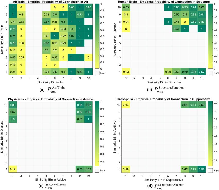
The diagram in Fig. 4 illustrates the process of node-pairs similarity calculation in SimBins. The main source
of information are the structure of the target and auxiliary layers. The train and test sets are derived from the
target layer including both links and non-existent link (the test set is later used for evaluation). The rest of the
process includes partitioning of the train set (U ′ ) according to the base similarity scores in T , A and connected-
ness in A. Accordingly, intra-layer and trans-layer connection probabilities of each partition (bin) is calculated
and fed to the final SimBins scoring Eq. (25).
Experimental results. The link prediction performance on9 different datasets, a total of 29 network layers
forming 52 layer-pairs has been reported based on both AUC (Table 2) and Precision (3) evaluation metrics.
The evaluation metrics are the mean over 100 iterations with train ratio set to 90% as described in ‘Evaluation
Method’ section. Four base measures comprising local, global and quasi-local indices have been incorporated
i.e., RA, CN, ACT and LPI that were introduced in ‘Base Similarity Measures’ section. SimBins (SBA T ≡ SB
T,A) is
Scientific Reports | (2021) 11:13242 | https://doi.org/10.1038/s41598-021-92427-1 12
Vol:.(1234567890)www.nature.com/scientificreports/
Figure 4. An overview of simbins method.
compared with baseline methods including scoring based on similarity in the target layer (ST ) and simple addi-
tion of similarity scores of the target and auxiliary layers (ST + SA).
In Table 2, for each base measure, the highest mean AUC is shown in bold and, for each duplex (all 52
rows), the highest AUC among all of the methods (independent from the base measure) is highlighted with an
underscore. SimBins dominates other baseline methods and proves to be an effective multiplex link prediction
method due to several reasons: (i) Most of the time, SimBins is superior to the other baseline methods (i.e., bold
entries). This can be further verified with the fact that SimBins achieves higher average of all mean AUCs (the
last row of the table) (ii) In a large fraction of duplexes (37 of 52), the overall best mean AUC belongs exclu-
sively to SimBins (in 6 other duplexes, SimBins achieves the best performance alongside another method, non-
exclusively) (iii) SimBins performs better than the single-layer method (or ST ) in most of the cases whereas for
similarities addition method (ST + SA) this is less frequently observed; meaning our method is capable of using
other layer’s information effectively. And, SBT,A is more robust against deceptive signals compared to ST + SA.
Consider Drosophila for example. The slightly negative correlation between similarity in the auxiliary layer
(Suppressive) and connection probability in the target layer (Additive), as previously discussed on (Fig. 2-d), has
caused performance reduction for ST + SA whereas SimBins still performs as good as—if not better than—ST .
A similar outcome can be observed for NTN and London Transport, more clearly when ACT is used as the base
similarity measure. In CS-Aarhus, where Facebook is the target layer, both ST and ST + SA perform even worse
than random scoring (expected 50% AUC) while SimBins keeps the performance up about 70 − 80%. As the
last row indicates, the average mean AUC of SimBins is higher than both other baseline methods, no matter the
choice of base measure.
There exist occasions in which SimBins cannot improve the link prediction performance compared to the
base similarity measure. Specifically, Drosophila which the absence of inter-layer correlation as discussed ear-
lier is the underlying reason. And, in London Transport, node multiplexity is far too low as shown in Table 1.
Consequently, very few nodes are shared among different layers that makes utilization of structural similarities
between layers a hard task.
The above discussion holds true for Adamic-Adar9, Preferential Attachment8, and LRW15 similarity measures,
as we have performed similar experiments which led to resembling results, but we have avoided bringing the
corresponding details for the sake of brevity.
Interestingly, the results appear to suggest that choosing LPI as the base similarity measure, leads to the best
overall performance in most of the multiplex networks. Using LPI as the base similarity measure for SimBins
gives the best performance with average mean AUC of 85.0% for all 52 duplexes under study.
The evaluation of methods based on Precision metric as reported in 3, confirms our earlier discussions. This
metric measure quantifies the quality of top entries of the sorted list of unobserved links while AUC consid-
ers the quality of the ranking in the whole list. Here, also SimBins is superior compared to other two baseline
methods. Specifically, in 38 duplexes out of 52 the best performance based on Precision metric is for SimBins
while in 2 duplexes it shares the best performance with another baseline method. So, the results of Tables 2 and
3 confirm the superiority of SimBins over baseline methods regardless of the choice of base similarity measure
and evaluation metric and also suggest that using SimBins along with LPI as the base similarity measure leads
to the best performance.
Finally, we compare SimBins with three state-of-the-art methods, namely, YaoPL, YaoGL38, and SameiHP39.
An introduction to these methods is given in ‘Related Works’ section. The scoring schema of these methods can
be summarized as Eq. (26). The base similarity measure used in these methods (ST and SA for the target and
auxiliary layers T and A respectively) is LPI for the two former methods and HP for the latter. Moreover, the layer
relevance measure (µT,A)is PCC for YaoPL and GOR for YaoGL and SameiHP. Based on the recommendation of
the authors, the parameter ϕ = 0.5 is considered. The results of the experiments are shown in Table 4.
Scientific Reports | (2021) 11:13242 | https://doi.org/10.1038/s41598-021-92427-1 13
Vol.:(0123456789)www.nature.com/scientificreports/
Target Auxiliary
layer layer RA CN ACT LPI
ST ST + SA SBA
T ST ST + SA SBA
T ST ST + SA SBA
T ST ST + SA SBA
T
Air Train 83.9 89.9 90.6 79.8 85.0 84.9 87.7 85.9 89.2 80.1 86.1 82.8
AT
Train Air 83.3 84.0 83.8 83.1 83.3 84.2 79.6 80.3 80.9 84.1 84.0 84.8
Chem-
70.6 79.0 80.3 70.6 78.5 80.3 64.7 65.8 69.6 76.6 82.4 83.0
Electric Mono
Chem-Poly 70.6 84.0 85.6 71.0 83.3 85.9 65.5 68.7 72.5 76.4 84.2 85.9
C. Chem- Electric 76.2 77.0 78.2 75.8 76.3 77.8 67.3 67.8 70.5 84.3 83.9 84.8
ELEGANS Mono Chem-Poly 76.2 87.3 90.8 75.7 85.4 91.7 68.4 73.4 89.0 84.1 88.3 89.9
Electric 85.8 85.9 86.5 84.0 83.9 84.5 72.3 72.0 73.9 86.3 86.1 86.3
Chem-
Poly Chem-
85.6 86.9 88.7 84.1 85.3 87.6 72.3 73.1 81.9 86.3 87.5 87.6
Mono
Suppres-
Additive 76.5 75.9 76.7 76.6 75.7 76.6 80.9 74.3 77.2 82.3 81.2 82.3
DM sive
Additive Suppressive 74.2 73.8 74.2 73.9 73.1 73.7 73.6 70.2 69.4 79.5 77.7 79.2
Structure Function 91.2 91.3 92.9 89.9 88.9 91.9 75.4 69.2 78.6 92.1 90.8 94.2
HB
Function Structure 86.0 88.8 89.9 85.6 88.5 89.9 68.9 72.5 79.9 89.0 90.0 91.0
Discuss 71.4 81.9 87.3 71.9 82.6 88.7 50.9 66.3 77.0 84.7 93.7 93.4
Advice
Friendship 71.6 78.0 81.3 72.1 78.4 81.8 50.0 58.0 62.2 84.6 89.5 89.6
PHYSI- Advice 75.2 81.3 87.2 74.6 80.7 87.3 52.7 61.8 74.1 83.4 91.6 91.7
Discuss
CIANS Friendship 74.6 81.2 84.6 74.0 80.1 84.8 51.9 62.1 67.9 83.9 90.5 90.3
Friend- Advice 69.9 77.6 80.9 69.8 77.5 81.2 56.3 57.3 66.9 77.9 86.6 87.1
ship Discuss 69.8 82.1 86.0 69.7 81.6 86.7 56.2 65.6 72.8 78.1 89.9 89.9
Financial 84.2 83.8 83.0 82.7 82.6 82.7 74.8 63.6 71.8 82.0 81.7 82.8
Com-
Operation 84.3 84.3 87.2 82.6 82.9 87.9 75.0 68.0 84.8 82.4 82.1 87.4
muni
Trust 84.0 84.1 89.4 83.3 81.2 88.9 73.6 71.3 82.6 82.0 81.3 86.8
Communi 91.5 92.1 90.7 90.5 78.6 90.0 52.7 40.6 68.7 89.7 77.8 87.9
Financial Operation 89.5 83.8 90.2 90.0 67.4 92.1 54.1 54.1 67.5 92.0 66.1 92.6
Trust 91.7 92.7 96.9 90.2 79.3 93.3 50.6 41.0 77.6 93.0 83.4 96.2
NTN
Communi 98.0 98.0 98.8 97.3 97.5 98.2 66.9 68.3 81.4 96.7 97.3 97.8
Opera-
Financial 98.2 97.9 98.2 97.3 97.3 97.2 67.1 58.8 73.9 96.7 96.7 96.8
tion
Trust 98.3 95.6 98.7 97.2 94.6 97.7 67.6 65.5 78.7 97.0 94.2 97.7
Communi 88.5 92.4 94.8 87.7 91.6 94.7 78.2 80.3 90.5 88.6 92.9 92.6
Trust Financial 88.5 88.3 88.5 87.5 87.4 87.5 77.9 67.4 80.6 88.5 88.4 88.7
Operation 88.6 88.3 91.6 88.1 86.9 92.1 78.3 71.3 84.1 88.3 85.5 91.0
Over-
53.2 53.2 55.0 53.4 53.4 55.0 53.3 47.1 61.0 58.0 59.6 59.9
Tube ground
DLR 53.5 53.4 53.5 53.7 53.7 53.7 54.7 50.4 50.1 57.7 57.6 57.8
LONDON Over- Tube 49.9 50.3 55.6 49.9 50.4 56.0 49.1 51.7 81.5 49.9 55.3 55.0
TRANS ground DLR 49.9 49.9 49.9 50.0 49.9 50.1 49.7 48.9 56.0 49.9 49.7 49.9
Tube 52.8 53.2 50.4 53.0 53.6 49.8 56.5 58.5 64.3 52.3 53.2 53.2
DLR Over-
52.2 52.2 49.8 52.8 52.7 50.4 57.9 57.4 50.6 53.0 52.8 53.0
ground
Facebook 94.7 93.3 94.8 94.7 91.0 94.7 83.5 61.5 84.0 93.9 89.5 94.5
Co-author 95.4 95.3 95.3 93.5 93.4 93.4 83.4 56.0 83.6 94.2 94.1 94.4
Lunch
Leisure 94.5 94.2 94.9 94.0 93.9 94.4 82.8 68.7 85.8 93.5 93.2 93.9
Work 94.7 94.7 95.5 93.8 93.3 95.3 84.1 82.3 88.1 94.6 92.9 95.9
CS- Lunch 93.5 90.5 93.8 92.8 90.3 92.5 43.6 51.6 78.8 95.0 91.3 95.3
Facebook
AARHUS Co-author 92.5 92.1 92.9 93.2 93.1 93.6 42.7 47.3 74.7 94.7 94.6 94.8
Co- Lunch 73.0 92.2 89.7 69.1 91.5 91.2 45.6 58.9 72.0 73.3 92.0 94.8
author Facebook 72.9 70.5 79.6 69.8 66.2 73.6 43.1 62.2 68.6 73.3 71.9 81.2
Leisure Lunch 82.8 90.5 90.2 81.4 89.2 89.7 58.9 75.1 81.8 81.7 89.1 89.5
Work Lunch 88.1 91.0 91.3 86.2 89.9 89.9 71.6 83.2 82.0 85.4 89.4 89.4
Continued
Scientific Reports | (2021) 11:13242 | https://doi.org/10.1038/s41598-021-92427-1 14
Vol:.(1234567890)www.nature.com/scientificreports/
Target Auxiliary
layer layer RA CN ACT LPI
ST ST + SA SBA
T ST ST + SA SBA
T ST ST + SA SBA
T ST ST + SA SBA
T
Colocaliza-
62.9 64.3 65.8 62.9 64.3 65.7 51.7 50.1 68.2 73.1 75.9 75.9
tion
Direct Physical 62.9 71.8 76.8 63.0 70.1 76.5 51.8 52.6 75.9 74.0 82.2 85.5
SACCH- Synthetic 62.8 69.8 70.9 62.8 69.6 70.9 50.9 50.2 69.3 73.3 80.4 80.4
POMB
Association 63.1 63.7 64.3 63.0 63.7 64.2 52.0 51.6 72.8 73.4 74.6 74.6
Physical Direct 77.8 78.4 79.4 77.4 78.0 79.0 69.4 57.8 76.3 88.4 89.5 88.6
Synthetic Direct 80.3 81.5 82.2 80.3 81.5 82.3 65.2 54.2 82.8 90.9 92.1 92.1
AVERAGE AUC 78.5 81.0 82.8 77.8 79.4 82.4 63.7 62.9 75.1 81.6 82.9 85.0
Table 2. Average AUC over 100 iterations for the networks under study. Each row shows the performance
of link prediction methods on a duplex subset of a multiplex network grouped by the corresponding base
similarity measure in use. Columns show the average AUC over 100 iterations for the prediction methods
ST (similarity score of only the target layer), ST + SA (addition of similarity scores of the target and auxiliary
layer), SBA
T ≡ SB
T,A (SimBins).
T,A T
Sx,y = (1 − ϕ)Sx,y + ϕµT,A Sx,y
A
m (26)
Clearly, SimBins achieves the best performance (85.0%) in term of average mean AUC over all 52 duplexes.
Also, in 25 duplexes SimBins is the best performing method (the best in 18 cases and sharing the best perfor-
mance in 7 cases with another method) while the second best is SameiHP with the best performance in 13
duplexes. It should be also noted that SameiHP method has large fluctuation across different networks and the
lowest average mean AUC. So, using SimBins based on LPI is our choice that performs well across diverse set
of multiplex networks.
Complexity analysis. Consider a duplex network G(V , E [1] , E[2] ; E[i] ⊆ V ×V ), mi = |E [i] |∀i ∈ {1, 2}
where layer 1 is the target, and layer 2 is the auxiliary layer. Let O(θ) be a representative of computational com-
plexity for the base similarity measures. The similarity of node pairs in both layers is needed for subset U ′ of
U = V × V as formulated in ‘Partitioning Node Pairs (Binning)’ section. Therefore, the computing complexity
of measuring similarities is O( i=1,2 θmi ). Partitioning U ′ into equal-depth bins requires sorting of similarities,
consequently it would have complexity of
i=1,2
i log mi ). Total estimation complexity of intra-layer and
O( m
trans-layer connection probabilities is O i=1,2 mi bi where bi is the number of bins in corresponding layer.
And, estimation of probability of connection in all 2d-bins according to Eq. (24) would be of orderO(b1 b2 )
which is negligible w.r.t bounded number of bins. Accordingly, the total computational complexity of scoring
a node pair in SimBins would be O(m log m) where m is in the same order as m1 , m2 if the sparsity of multiplex
layers is comparable. This tolerable computing complexity indicates that SimBins can be scaled for usage in large
networks.
Notice that for obtaining a full ranking of propensity of links, SimBins, like the majority of link prediction
algorithms would need at least O(n2 ); n = |V | computations which is not easily scalable to very large networks
without pruning the n2 space. To be specific, for a full ranking, SimBins would have a computing complexity
of O(θn2 + m log m) in which O(θn2 ) is the dominating term in real-networks; meaning that SimBins imposes
minor overhead to the base similarity measures. This makes SimBins appropriate for using with large networks
like SaccPomb that we studied in this paper.
Discussion
In this manuscript, we explored the intra-layer and trans-layer connection probabilities in multiplex networks
and verified that in many real multiplex networks, connection probability within an arbitrary layer is correlated
with similarity in other layers of the same multiplex. We also observe that connectedness in one layer of the
multiplex, increases the probability of linkage in other layers. Subsequently, we developed a consolidated link
prediction model by incorporating information theory concepts for characterizing intuitions gathered from the
observed evidences.
The proposed method works on a pair of multiplex’s layers i.e., a duplex. Different ideas can be conducted
to extend it to use multiple layers’ topology for link prediction. Considering a target layer T and auxiliary lay-
ers A1 , . . . , AM ,
the simplest idea is to add up the SimBins scores for each possible layer pairs, symbolically
SBT,{A1 ,...,AM } = M i=1 SB
T,Ai where SBT,Ai is computed according to Eq. (25). The other—not as straightforward
as previous– idea is to compose and study bins of more than two dimensions. This extension, although more
systematic, might suffer from heavy sparsity of samples (imagine node pairs residing in 3d-bins).
Eventually, SimBins is compared with two baseline methods (base similarity measure in the target layer and
simple addition of similarities in target and auxiliary layers) and three state-of-the-art methods (YaoPL, YaoGL
and SameiHP) on 9 multiplexes. It is shown that SimBins outperforms the other two baseline methods in most
cases. Besides, it rarely performs worse than target similarity and is more robust to deceptive signals compared
to the simple addition of similarities. It is mentioned that in some networks, such as London Transport and
Drosophila, SimBins seems to be unprofitable as a result of massively condensed node pairs similarity distribution
Scientific Reports | (2021) 11:13242 | https://doi.org/10.1038/s41598-021-92427-1 15
Vol.:(0123456789)You can also read