Long term stability predictions of therapeutic monoclonal antibodies in solution using Arrhenius based kinetics
←
→
Page content transcription
If your browser does not render page correctly, please read the page content below
www.nature.com/scientificreports
OPEN Long‑term stability predictions
of therapeutic monoclonal
antibodies in solution using
Arrhenius‑based kinetics
Drago Kuzman1, Marko Bunc1, Miha Ravnik2,3, Fritz Reiter4, Lan Žagar5 & Matjaž Bončina1*
Long-term stability of monoclonal antibodies to be used as biologics is a key aspect in their
development. Therefore, its possible early prediction from accelerated stability studies is of major
interest, despite currently being regarded as not sufficiently robust. In this work, using a combination
of accelerated stability studies (up to 6 months) and first order degradation kinetic model, we are able
to predict the long-term stability (up to 3 years) of multiple monoclonal antibody formulations. More
specifically, we can robustly predict the long-term stability behaviour of a protein at the intended
storage condition (5 °C), based on up to six months of data obtained for multiple quality attributes
from different temperatures, usually from intended (5 °C), accelerated (25 °C) and stress conditions
(40 °C). We have performed stability studies and evaluated the stability data of several mAbs including
IgG1, IgG2, and fusion proteins, and validated our model by overlaying the 95% prediction interval
and experimental stability data from up to 36 months. We demonstrated improved robustness, speed
and accuracy of kinetic long-term stability prediction as compared to classical linear extrapolation
used today, which justifies long-term stability prediction and shelf-life extrapolation for some
biologics such as monoclonal antibodies. This work aims to contribute towards further development
and refinement of the regulatory landscape that could steer toward allowing extrapolation for
biologics during the developmental phase, clinical phase, and also in marketing authorisation
applications, as already established today for small molecules.
Generation, evaluation, and interpretation of stability data of a pharmaceutical product are key aspects of drug
development1,2. During early technical development, stability data inform several important decisions, such as
formulation selection, the selection of primary packaging materials or defining the manufacturing process. In
addition, stability data are the basis for setting the shelf-life of a product, i.e. the period in which the quality of a
product has to remain within pre-set and well-justified shelf-life specifications. Obtaining real-time stability data
is very time-consuming and is a bottleneck of early technical development. Speeding up the process with acceler-
ated conditions (e.g. higher temperature) has been therefore attempted many times but with limited success in
accurate prediction3–8. Therefore, achieving robust and reliable long-term prediction of stability (usually several
years) from accelerated stability (usually a few months) is of major scientific and applied interest. Establishing
robust prediction approaches could allow for use of accelerated and stress conditions to determine the shelf-life
(safety) of a product beyond the period covered by actually measured and tested stability data.
Biologics like monoclonal antibodies, bispecific antibodies and fusion proteins are susceptible to a variety of
chemically- and temperature-induced structural changes2. For example, chemical changes of amino acid residues,
such as deamidation of asparagine and glutamine or oxidation of methionine or tryptophan can induce structural
changes in the overall protein structure, potentially leading also to changes in physical stability1,9,10. Both chemical
and physical degradation might compromise biological activity and safety of the b iologic11.
In early technical development of biologics, the risk-based predictive stability (RBPS), i.e. the prediction
of stability behaviour and the practice of extrapolation to support development milestones, is a company’s
internal decision. During the clinical development phase of biologics (and within clinical trial applications)
limited extrapolation is used and accepted by health authorities (HA) w orldwide12,13. Differently, in marketing
1
Biologics Drug Product, Technical Research and Development, Global Drug Development, Novartis, Lek D.D.,
Kolodvorska 27, 1234 Mengeš, Slovenia. 2Faculty of Mathematics and Physics, University of Ljubljana, Ljubljana,
Slovenia. 3Josef Stefan Institute, Ljubljana, Slovenia. 4Regulatory Affairs CMC, Global Drug Development, Novartis,
Sandoz GmbH, Kundl, Austria. 5Revelo d.o.o., Ljubljana, Slovenia. *email: matjaz.boncina@novartis.com
Scientific Reports | (2021) 11:20534 | https://doi.org/10.1038/s41598-021-99875-9 1
Vol.:(0123456789)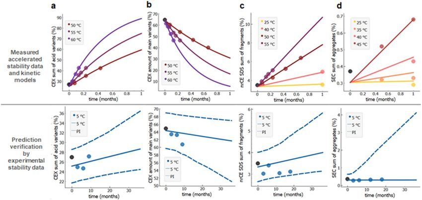
www.nature.com/scientificreports/
authorisation applications and in the commercial phase, extrapolation is not accepted for b iologics14. In the
majority of cases, for clinical trial submissions, long-term stability testing is also performed and included in the
submissions although some companies report using reduced protocols with fewer time points and conditions15,16.
For small molecule drugs, the prediction of stability behaviour is based on accelerated stability data obtained at
different temperatures and humidity levels. Experimental data are described by a kinetic model and expanded
Arrhenius equation which allows prediction of long-term stability. Such predictions are for small drugs usually
performed in accelerated stability assessment p rogram17–19. However, the prediction of stability of biologics is
still very limited and calculated by a classical approach using linear extrapolation. In clinical trial applications,
regulatory expectations for risk-based predictive stability of biologics allow extrapolation for the same period as
the available experimental data but not for more than 12 m onths12. Introducing RBPS into the development of
biologics would have similar advantages as in small molecules. In particular, extensive time saving by perform-
ing stability studies at higher temperatures and predicting stability at the intended storage temperature. This
approach allows also shelf-life estimation, quick evaluation of formulation and primary packaging, evaluation
of comparability for DP or DS process changes, evaluation of stability for a wide range of storage conditions and
more15. In addition, temperature excursions during storage or transport can be e valuated20.
It is considered that long-term stability predictions from accelerated stability data are usually not possible
for biologics due to the complexity of temperature, time and concentration-dependent modifications. When
studying aggregation, researchers either found non-Arrhenius behaviours3–6 or Arrhenius behaviour was very
limited to narrow temperature and concentration i ntervals7,8. However, recent studies indicated the possibility
to predict long-term aggregation profiles from accelerated stability data and some selected biophysical param-
eters by non-linear models, i.e. artificial neural networks21 or other multivariate approaches21,22. Arrhenius
behaviour was also demonstrated for vaccine potency to be utilised to manage stability after a process c hange23,
and to accurately predict long-term s tability20. Long-term profiles of vaccine antigenicity that were predicted
by Arrhenius kinetic analysis of six months of accelerated stability data were verified with up to three years of
stability experimental d ata20.
In this article, we demonstrate accurate long-term (up to 3 years) stability prediction of multiple quality
attributes for several therapeutic monoclonal antibodies and fusion proteins from short-term (up to 6 months)
accelerated stability data combined by applying kinetic modelling using the Arrhenius equation. Specifically, we
tested stability indicating quality attributes like purity, potency, aggregation, fragmentation and charge profile
for five monoclonal antibodies and one fusion protein. Prediction of three years stability profiles at intendent
storage condition was verified by experimental data: 96% of experimental data that were not used for building
the model, lie within the calculated prediction intervals that were approximately three times narrower than
the width of generic shelf-life specifications at the three year time point. More generally, this work is aimed to
underlay the relevance and applicability of using a combination of short-term accelerated stability studies and
kinetic modelling (beyond the currently used linear extrapolation) in the development of therapeutic monoclo-
nal antibodies. This is of major interest to the biopharmaceutical industry and for general society as it enables
shorter development periods of novel advanced biologics.
Materials and methods
Materials. All tested protein solutions were manufactured at Lek d.d. (member of Novartis), Mengeš, Slo-
venia and include IgG1 molecules adalimumab and rituximab, IgG2 molecule denosumab and mAb1 (IgG1)
and mAb2 (IgG2) molecules in development and fusion protein etanercept. Stability studies on rituximab were
done at protein concentration of 10 mg/mL. Protein was formulated in an innovator’s formulation, i.e. 0.7 mg/
mL polysorbate 80.9 mg/mL sodium chloride and 5.25 mg/mL citric acid monohydrate at pH 6.5. Stability stud-
ies on adalimumab were done at protein concentration of 50 mg/ml. Protein was formulated in design around
formulation comprised of 3.36 mg/mL adipic acid, 0.25 mg/mL citric acid monohydrate, 12 mg/mL mannitol,
1 mg/mL polysorbate 80 and 6.16 mg/mL sodium chloride at pH 5.2. Stability studies on denosumab were done
at 70 mg/mL. Protein was formulated in an innovator’s formulation, i.e. 1.08 mg/mL acetic acid, 46 mg/mL
sorbitol, 1 mg/mL PS20 at pH = 5.2. Stability studies on etanercept were done at 50 mg/mL. Protein was formu-
lated in design around formulation comprised of 0.786 mg/mL citric acid, 13.52 mg/mL sodium citrate, 1.5 mg/
mL sodium chloride, 10 mg/mL sucrose and 4.6 mg/mL lysine at pH 6.3. These four formulations are Novartis’
final drug product formulations identified as the most appropriate during the early drug product development.
Stability predictions for this four proteins were made also for different batches of the same molecule where the
batch represents a protein with uniform character and quality, within specified limits, and is produced according
to a single manufacturing order during the same cycle of manufacture. Variability between batches originates
from the production process. Stability studies on proteins in development mAb1 and mAb2 were done at protein
concentrations ~ 5 mg/mL (mAb1) or ~ 150 mg/mL (mAb2). Proteins were formulated in different formulations
and pH values between 5.5. and 7.0. All formulations were filled in different sizes of type I glass vials.
Chemicals for formulation preparation were of pharmaceutical grade, while chemicals and reagents for
chromatography and electrophoresis were of HPLC grade.
Analytical methods. The development of liquid dosage forms of biologics is mainly based on stability stud-
ies that are performed at accelerated ((25 ± 2) °C/(60 ± 5)% r.h.) and stress temperature ((40 ± 2) °C/(75 ± 5)%
r.h.) whereas the intended commercial storage temperature is between 2 and 8 °C (we will use 5 °C throughout
the article for simplicity reasons) with shelf-life usually between 2 and 3 years. Stability studies are performed
at 25 °C and 40 °C in order to speed up changes in the quality attributes of the protein that can be detected by
state-of-the-art analytical methods and save time spent for development. According to ICH guidelines stability
indicating quality attributes of the protein and analytical methods are defined by force degradation studies that
Scientific Reports | (2021) 11:20534 | https://doi.org/10.1038/s41598-021-99875-9 2
Vol:.(1234567890)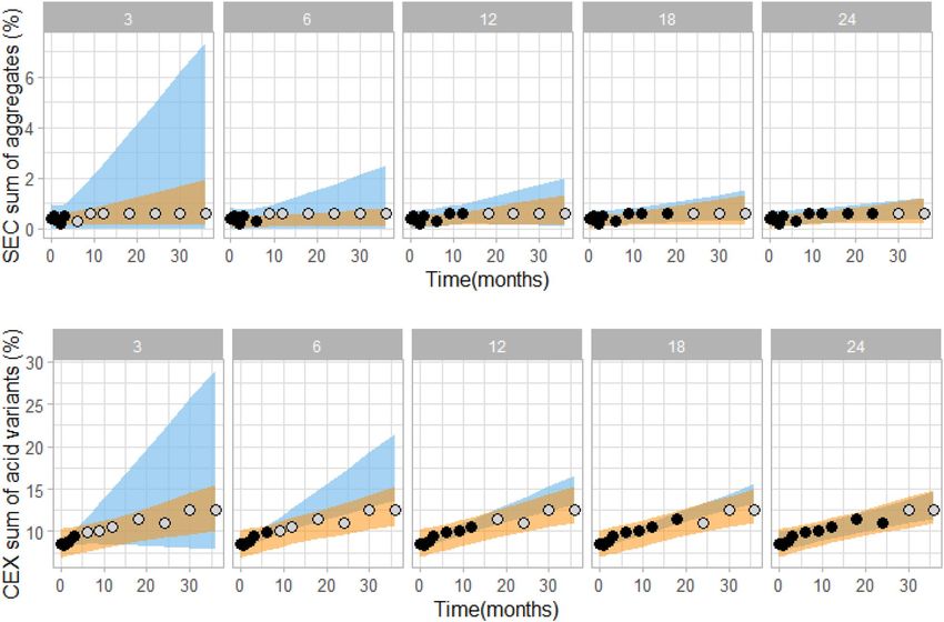
www.nature.com/scientificreports/
are designed in a way to identify likely degradation mechanisms24. As such, the intrinsic stability of the molecule
is determined and the analytical methods indicating stability are validated. When developing a drug product for
biologics, modifications/changes of different quality attributes are assessed. They can be divided into two groups:
concentration-independent and concentration-dependent. The most prominent concentration-independent
modifications are chemical modifications such as oxidation, (de)amidation, isomerisation, etc. These modifica-
tions are usually detected by peptide mapping (PepMap), imaged capillary isoelectric focusing (iCIEF), capillary
zone electrophoresis (CZE), cation exchange chromatography (CEX) and reverse phase chromatography (RPC).
The second type of concentration-independent modification is fragmentation that is detected by SDS capillary
electrophoresis (CE-SDS). Concentration-dependent modifications are aggregation monitored by size exclusion
chromatography (SEC) and formation of subvisible particles monitored by light obscuration (LO) or micro
flow imaging (MFI) and formation of visible particles detected by visual inspection. Bioactivity, which is typi-
cally monitored by cell-based assays and by functional tests like surface plasmon resonance (SPR) or bio-layer
interferometry (BLI), is impacted by the combination of the above-mentioned modifications. Frequently, purity
is reported in addition. It is determined as the amount of the main peak assessed by iCIEF, CZE, CEX, CE-SDS
or SEC.
Size exclusion chromatography (SEC). SEC analysis was performed on Agilent 1260 HPLC or Acquity
H-class UPLC instrument using Waters Acquity BEH200 SEC, 1.7 µm, 4.6 mm × 150 mm column or similar.
Mobile phase was 50 mM Na2HPO4/NaH2PO4 and 400 mM NaClO4 at pH 6.0 or 150 mM KH2PO4/K2HPO4 at
pH 6.5. Monomer and aggregate peaks were detected by measuring absorbance at 210 nm. Chromatograms were
analysed using Empower or Chromeleon software. Size of aggregates was determined from a calibration curve
obtained from analysis of molecules of known molecular weights: thyroglobulin (669 kDa), IgG (150 kDa) and
holo-transferrin (80 kDa). Accuracy of the measured amount of aggregates is between 0.05 and 0.1% while the
amount of main peak (purity) is between 0.1 and 0.2%.
Cation exchange chromatography (CEX). CEX analysis was performed on Agilent 1260 HPLC instru-
ment usually using MabPac SCX-10, 10 µm, 4 mm × 250 mm column from Thermo Scientific. Mobile phase
A was 5.8 mM MOPSO, 4.4 mM Bicine, 12.2 mM CAPSO, 0.6 mM CAPS, pH 6.6, while mobile phase B was
12 mM MOPSO, 4 mM Bicine, 1.2 mM CAPSO, 5.8 mM CAPS, pH 11.5. Percentage of mobile phase B was
increased from 15.9% to 63.7% in 26 min. Alternatively, MabPac SCX-10, 3 µm, 4 mm × 50 mm column from
Thermo Scientific was also used in combination with mobile phase A composed of 5 mM TAPS, 5 mM CAPSO,
10 mM NaCl at pH 7.8 and mobile phase B composed of 5 mM TAPS, 5 mM CAPSO, 10 mM NaCl at pH 10.2.
Percentage of mobile phase B was increased from 0 to 55 and 55 to 90% in 1 and 27 min, respectively. Absorb-
ance chromatograms were analysed at 280 nm using Empower or Chromeleon software. Accuracy of measured
amount of acidic, basic variants and main peak (purity) is between 0.5 and 1.5%.
SDS capillary electrophoresis (CE‑SDS). CE-SDS analysis was performed by PA 800 Plus instrument
from Sciex. Typically, bare fused-silica capillary with 50 μm of internal diameter and 20 cm long was used for
the separation. SDS gel and SDS sample buffers were obtained from Sciex. Non-reducing conditions were always
used. Protein-SDS complex was alkylated with iodoacetamide or N-ethylmaleimide in a 45–70° C water bath
for 10 min. After samples were cooled, they were electrokinetically introduced into the capillary and separated
by applying constant voltage. Absorbance electropherograms were analysed at 210 nm using Empower or Karat
software. Accuracy of measured amount of fragments is between 0.2 and 0.3% while for the amount of main
peak (purity) is between 0.3 and 0.5%.
Bioactivity. In the complement-dependent cytotoxicity (CDC) test25, Raji B cells (isolated from a patient
with Burkitt’s lymphoma, from American Type Culture Collection (ATCC)) are incubated with different protein
concentrations and a fixed concentration of rabbit complement. Concentration-dependent killing of the Raji
cells is analysed after 2 h where viability of the cells is measured with indirect determination of ATP concentra-
tion (by measuring luminescence produced by the ATP-consuming luciferin-luciferase system). In the case of
tumor necrosis factor-alpha (TNFα) antagonists such as etanercept and adalimumab reporter gene assay was
used as descibed in 26. Activity of the protein’s test sample is determined by comparison to a reference standard.
The samples and the standard are normalised on the basis of protein content. Relative potency is then calculated
using a parallel line assay according to the European Pharmacopoeia. Accuracy of measured relative potency is
around 10%.
Kinetic model. Kinetic models of protein processes are composed from dynamic rate terms of quality
attributes and the empirical Arrhenius equation27 that describes the temperature dependence of rate constant.
Quality attributes considered are purity and sum of impurities, i.e. fragments, charge variants and aggregates.
When studying stability of the drug product from the fragmentation standpoint, we are usually interested in the
sum of fragments, meaning that the apparent chemical reaction can be approximated as A → B (see Fig. 1, top
scheme). The same reaction scheme was applied also when assessing chemical modifications (middle scheme).
We can monitor single amino acid residue modification with PepMap or the sum of acid or basic variants by
iCIEF, CZE or CEX. The latter approximation was reported to have been successfully used for describing chemi-
cal modification of a single amino acid residue28–30. In the examined cases, aggregation was monitored by the
SEC method and the sum of aggregates was determined. Dimers were the most abundant species among the
aggregates for all tested proteins at all time points. Thus, the fastest pathway was formation of dimers, especially
at T < 40 °C, where only minor amounts of larger aggregates were detected. Chromatogram overlays of mAb1,
Scientific Reports | (2021) 11:20534 | https://doi.org/10.1038/s41598-021-99875-9 3
Vol.:(0123456789)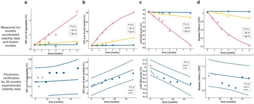
www.nature.com/scientificreports/
Figure 1. Simplified scheme of protein degradation and aggregation pathways. Top scheme: fragmentation,
middle scheme: chemical modifications, bottom scheme: aggregation. Figure made in PowerPoint 2016
(Microsoft, Redmond, WA, USA).
which show total area under the curve did not change with time even at 55 °C storage temperature, is provided
in Figure S1, while the same was observed for other mAbs for all conditions tested as well. This finding for exam-
ined monoclonal antibodies largely simplifies the model for aggregation, which can be described by the chemical
reaction 2A → B2 (bottom scheme in Fig. 1). We are aware that aggregation pathways can be more c omplex31–33
and can vary depending on temperature, time, protein type, concentration, formulation, process and more3,34.
Depending on the conditions, we may observe native or non-native aggregation that proceeds via different reac-
tive intermediates towards different oligomers (dimers, trimers, etc.), soluble polymers and precipitates35. Nev-
ertheless, if aggregation conditions are carefully chosen, the process can be successfully described using the
simple model mentioned.
In our kinetic modelling, we assume apparent one-step irreversible chemical reactions A → B and 2A → B2
which can be described by equations:
d[A]
= k(T)[A]n (1a)
dt
d[Bi ]
= k(T)[A]n (1b)
dt
Equation (1a) describes how concentration of A changes over time t and Eq. (1b) how concentration of B i
(i = 1 or 2, respectively) changes over time t, both with respect to reaction order n, temperature-dependent rate
constant k(T). A → B and 2A → B2 reactions are first (n = 1) and second (n = 2) order, respectively. Importantly,
these chemical reactions should be understood as ‘apparent’ because they do not necessarily correspond to the
actual dynamical processes in our protein systems, i.e., these apparent reactions should be understood as effec-
tive phenomenological dynamics observed in experiments.
In order to predict stability at different temperatures (in the temperature range from 5 to 60 °C, as relevant
for our monoclonal antibodies), we use the Arrhenius e quation27 that empirically describes temperature depend-
ence of rate constant, k(T)
Ea
k(T) = Af e− RT (2)
where Af represents the frequency factor and Ea the activation energy. In this case k(T) represents the degradation
rate constants that applies to a particular quality attribute of the molecule, such as aggregation, fragmentation,
chemical modifications and bioactivity. Based on the assumption explained below we approximated all kinetic
processes as first order chemical reactions. The combination of Eqs. (1a) or (1b) and (2) thus results in simple
first order degradation kinetic model, namely for purity quality attributes:
[A](t, T) = [A0 ]e−k(T)t (3)
and for the (sum of) impurities by taking into account that [A] + [B] is total concentration:
[B](t, T) = 1 − (1 − [B0 ])e−k(T)t (4)
We should comment that we use first order degradation kinetic model to describe degradation and aggre-
gation processes for the following reasons: We use temperature conditions and time intervals (i) where only
one degradation/aggregation pathway d ominates34, (ii) where relatively small changes in the quality attributes
of the protein are detected, usually up to 20% in 3 months at 40 °C, (iii) where the amount of formed higher-
order aggregates not detected by SEC is n egligible33, (v) where only aggregates detected by SEC, among which
dimers are the most abundant, are considered, thus more complex mechanisms of nucleation and growth can
be omitted3, and (iv) aggregation is studied at constant protein concentration, therefore second order kinetics
can be approximated by first order degradation kinetic model.
Scientific Reports | (2021) 11:20534 | https://doi.org/10.1038/s41598-021-99875-9 4
Vol:.(1234567890)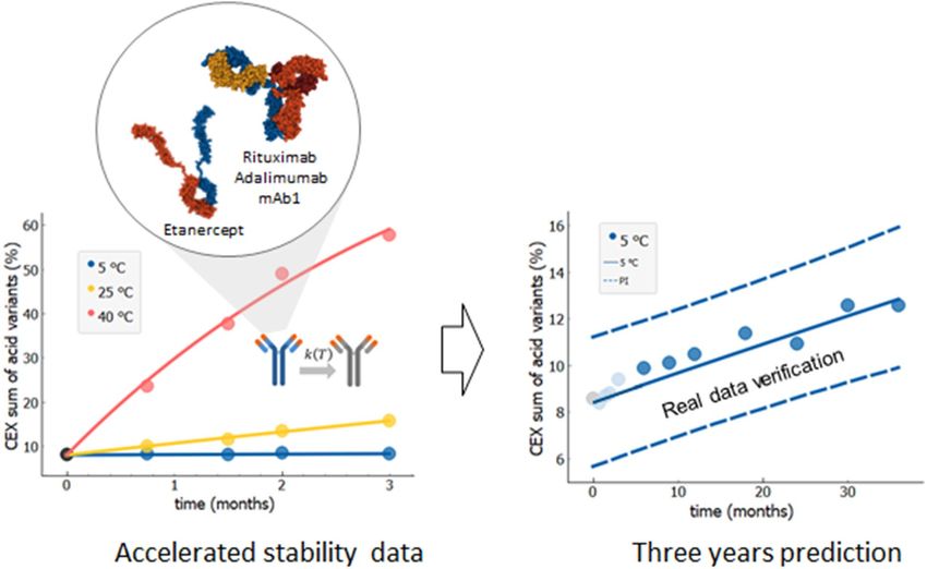
www.nature.com/scientificreports/
Kinetic model fitting and calculation of prediction intervals. Kinetic model parameters are calcu-
lated using data from the accelerated stability study for a single batch. The set of experimental stability data for
a given batch of biologics thus consists of time interval (up to 6 months), temperature conditions, and analytical
measurements of sample quality profile, including bioactivity.
Using this data we simultaneously fit a single model, not only in time, but also for different temperatures
(using Arrhenius relation), which crucially contributes to the robustness of the fitting. Precisely this multi-
parameter fitting allows for reliable and robust extrapolation in time (and also in temperature) using the fitted
kinetic model, well beyond the measured range of the parameter space. A single analytical measurement of
sample pulled at t = 0 was initial experimental value for all different temperatures datasets.
The kinetic model is fitted to a given set of experimental stability data numerically, using non-linear least-
squares optimisation, which minimises the sum of squared residuals SSres:
SSres = (yi − pi )2 (5)
i
where yi are the actual measurements and pi the calculated model points. Model parameter fitting was done in
Python using the SciPy library’s curve_fit function set to the “dogbox” method36. To improve the numerical
stability, we used a different parametrization of Eq. (2), solving the problem for parameters Ea and k(Tref ):
− ERa ( T1 − Tref
1
k(T) = k(Tref )e
)
(6)
We chose the intended storage temperature (5 °C) as Tref , so the solution of the problem directly provides
the rate of degradation at this condition, while the rate at other temperatures can be computed using the model.
To verify the quality of the model fit and compare it across different data sets we used the coefficient of deter-
mination (R2), which is a normalised score with the maximum value of 1, achieved when the model fits the
experimental data perfectly:
SSres
R2 = 1 − (7)
SStot
where SStot is defined as:
SStot = (yi − y)2 (8)
i
To further enhance and, more importantly, evaluate the quality of our extrapolation, we use Monte-Carlo
simulations to construct prediction intervals for the kinetic model. From a given set of experimental data we
generate an additional 399 sets of perturbed data, where we add random variation (noise) to the original meas-
urements sampled from a Gaussian distribution with zero mean and standard deviation set to the measuring
equipment’s specified error (equal to method accuracy noted in the description of each analytical method). We
repeat the parameter estimation and prediction for the desired conditions for each perturbed set to obtain a
distribution of predictions. The 2.5th and 97.5th percentiles give us the 95% probability confidence interval, while
the 95% probability prediction interval additionally accounts for the dispersion due to measurement errors and
is computed as in 37. The upper and lower bounds are computed separately as the interval can be asymmetric.
The described regression and extrapolation are established approaches when dealing with fitting the non-linear
model functions to experimental d ata38,39. The calculations were implemented as a custom widget within the
Orange data mining framework (https://orangedatamining.com/)40.
Linear regression. According to ICH guidelines41, linear regression is applied for modelling of stability
profiles and for shelf-life calculations. Linear extrapolations are accepted as well by health authorities to support
clinical development phase of drugs12. In our work, linear extrapolation is used to allow for comparison with our
improved kinetic modelling. The coefficients, intercept and slope, of the linear model were calculated by using
measured levels of quality attributes at given pull points for samples stored at intended storage condition (5 °C).
Coefficients and 95% prediction intervals were calculated by applying lm and predict functions from the stats
library of R42.
Verification of model extrapolation against experiments. As the key final verification of our in-
time extrapolation (i.e. prediction) of the changes of quality attributes, we compare the calculated prediction
intervals with actual full measured stability data (over 3 years) that is available at time of writing. Verification is
calculated/denoted as number of points lying within the 95% probability prediction interval among all experi-
mental stability data points. Short-term accelerated or intended condition stability data (of 6 months) used in
model fitting are excluded from this verification pool of data. The verification of model extrapolation against
long-term experimental stability data is used here to prove the correctness of our methodology; however, the
idea is precisely that these long-term experimental stability studies may not be needed anymore, if using more
advanced kinetic modelling beyond linear extrapolation.
Results
Long‑term stability prediction from accelerated stability data. Figure 2 shows the exemplary
long-term (36 months) stability prediction based on accelerated stability data (3 months) and kinetic modelling
using the Arrhenius temperature dependence of kinetic rates. Specifically, the image shows results for rituximab
molecule and the prediction for increase of the sum of acidic variants. We used experimental data for 3 months
Scientific Reports | (2021) 11:20534 | https://doi.org/10.1038/s41598-021-99875-9 5
Vol.:(0123456789)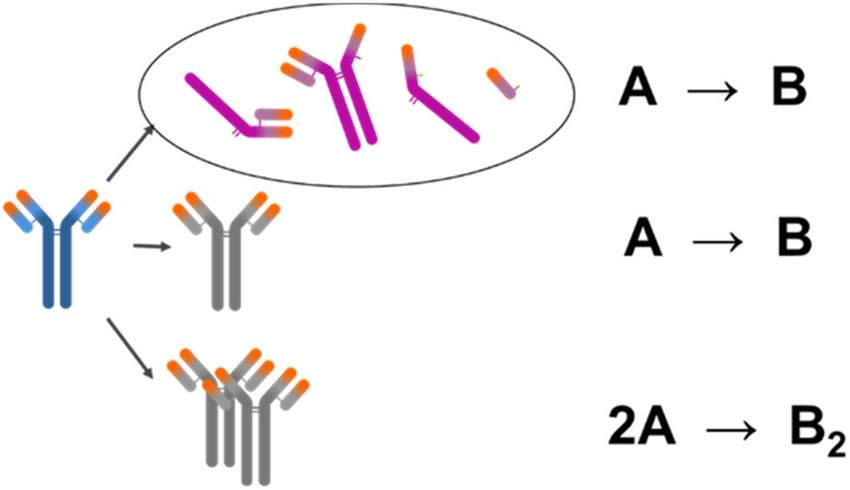
www.nature.com/scientificreports/
Figure 2. Long-term (36 months) stability prediction based on accelerated stability data (3 months) and kinetic
modelling which included Arrhenius temperature dependence of kinetic rates. Accelerated stability data (left,
data points) are used to develop the kinetic model (left, full lines) to predict long-term stability at intendent
storage conditions (right). The 95% probability prediction interval designated by dashed blue lines is verified
by long-term experimental data not used in model fitting (right, dark blue data points). Stability prediction was
evaluated for three mAbs (rituximab, adalimumab and mAb1) and for one fusion protein etanercept. Shown
data points are values of sum of acid variants obtained by CEX, one of the stability indicating quality attribute,
measured for one batch of rituximab. Each point represents single measurement (N = 1). Measurement accuracy
SD = 1.5% was estimated by several measurements of control samples over multiple analytical runs. Protein
structures created using 1 HZH43, 1H3W44 and 3ALQ45 structures from RCSB PDB (rcsb.org)46 using Mol*47 and
Snagit (TechSmith, Okemos, MI, USA).
(Fig. 2, left, data points) and for three different temperatures (5, 25 and 40 °C), which were obtained within an
accelerated stability study. These experimental data were then fitted with the kinetic model by using Eqs. (4) and
(6) (Fig. 2, left, full lines). We fitted simultaneously all three measured temperatures. The 3-year prediction curve
for the change of selected quality attribute in time was determined, together with the 95% probability predic-
tion interval (Fig. 2, right, full and dashed lines, respectively). Finally, the prediction interval obtained from the
3 months accelerated stability data is validated against the long-term experimental data (Fig. 2 right, dark blue
data points), showing excellent agreement between the prediction and actual measurements, with all measured
data points within the prediction interval and very close to the prediction curve.
Prediction of changes of multiple stability quality attributes. Figure 3 (upper panels, data points)
show measured data from (accelerated) six months stability study of the key stability indicating quality attributes
of rituximab (same batch as above). These accelerated stability data were analysed—i.e. fitted and extrapolated
separately for each stability quality attribute: sum of aggregates by SEC (Fig. 3a), sum of acidic variants by CEX
(Fig. 3b), purity by nrCE-SDS (Fig. 3c), and complement-dependent cytotoxicity activity CDC since this is the
main mode of action of rituximab. (Fig. 3d). The obtained stability profiles and prediction intervals for long-
term 36 month period (intended drug shelf-life) at intended conditions (5 °C) are shown on the lower panels of
Fig. 3 (full and dashed lines). Similarly as above, the predictions are validated against long-term experimental
stability data (Fig. 3, bottom panel, dark blue data points not used for model building), showing excellent agree-
ment with the predictions based on 6 months accelerated stability data. Furthermore, we verified whether first
order degradation kinetic model can be successfully applied to predict long-term stability profiles of sum of
aggregates for adalimumab, etanercept, denosumab and mAb1. As shown on Figure S2, 95% probability predic-
tion intervals encapsulate all experimental long-term stability data.
Improving robustness of kinetic model from accelerated data by goodness of fit and by tem‑
perature sub‑sampling. We assess the relevance and appropriateness of the chosen kinetic model using
only accelerated stability data. The most straightforward criterion that measures the appropriateness of the
Scientific Reports | (2021) 11:20534 | https://doi.org/10.1038/s41598-021-99875-9 6
Vol:.(1234567890)www.nature.com/scientificreports/
Figure 3. Long-term stability prediction of different stability indicating quality attributes for rituximab. (a) Sum
of aggregates by SEC (R2 = 0.92), (b) sum of acidic variants by CEX (R2 = 1.0), (c) purity by nrCE-SDS (R2 = 0.99),
(d) complement-dependent cytotoxicity activity (CDC) (R2 = 0.99). Accelerated 6 months experimental stability
data (upper panels, data points) are used for model parameter calculations (upper panels, full lines). Prediction
intervals (dashed blue lines in lower panels) are validated against the available long-term experimental data
(bottom panel, dark blue data points). All experimental data are from the single material batch. Measured value
at t = 0 is designated by a black solid circle.
applied kinetic model is the goodness of fit (R2) value as introduced in the Methods section. In the presented
study we achieved 0.9 < R2 < 1 in most cases, indicating good quality of fits. Note that observing low R2 indicates
either high values of measurement errors in the stability data or improper selection of the kinetic model.
The second criterion of model robustness is based on sub-sampling of the experimental accelerated stability
data, by joint fitting data from fewer selected temperatures. Typically, our accelerated stress stability studies are
performed at least at three different temperatures (e.g. see Fig. 3), and model fitting is performed with all acces-
sible short-term data (i.e. with all temperatures). However, to test the robustness, we include only subsets of
data (i.e. from fewer temperatures, minimal three temperatures) in fits and observe the obtained fit parameters
Ea and k(Tref ). If fitting results in the same model parameters for different subsets and the full set of data (all
temperatures), this indicates that the kinetic model is robust in the whole temperature range. For example, if
stability data is available for 5 °C, 25 °C, 40 °C and 50 °C temperatures one can get 5 different data subsets, where
minimally three different temperatures are included in a single data subset: {5 °C, 25 °C, 40 °C}, {5 °C, 25 °C,
50 °C}, {5 °C, 40 °C, 50 °C},{ 25 °C, 40 °C, 50 °C} and {5 °C, 25 °C, 40 °C, 50 °C}.
The described approach was confirmed by using mAb1 molecule stability data in temperature range up to
60 °C. Figure 4 shows activation energies as obtained from first order kinetic model fitting of different tempera-
ture data subsets. For charge variant analysis (Fig. 4a,b) and for fragmentation analysis (Fig. 4c,d) we have data
available for six storage conditions (5 °C, 25 °C, 40 °C, 50 °C, 55 °C and 60 °C) resulting in 42 different combina-
tions with at least three different temperatures in a subset. For sum of aggregates analysis (Fig. 4, panels e and
f) where additionally data for 35 °C and 45 °C temperatures are available, the number of combinations is 219.
The analysis of charge variants (Fig. 4a,b) resulted in very similar activation energy Ea values (approximately
25 kcal/mol) for all temperature sub-sampling combinations, including 60 °C condition. This clearly demonstrates
that first order degradation kinetic model for chemical modifications follows the Arrhenius relation across the
whole temperature range (5–60 °C) in the event of mAb1 molecule. In the fragmentation analysis (Fig. 4c,d),
Ea of 25 kcal/mol is obtained for all temperature combinations, except for subsets including 60 °C temperature.
Expectedly, in these subsets R2 was below the threshold level of 0.9. Collectively these two findings suggest that
at higher temperatures additional mechanisms of fragmentation are present, which are beyond the dynamics
covered in our (rather simple) kinetic model. The aggregation process (Fig. 4e,f) is even more complex involving
additional aggregation mechanisms already at T > 45 °C, reflected by increasing Ea above this temperature. Activa-
tion energy Ea for purity parameter (Fig. 4e) and sum of aggregates (Fig. 4f) is around 25 kcal/mol, the same as
in case of chemical degradation and fragmentation. Note that on Fig. 4, panels g and h, model verification results
for aggregation of fusion protein etanercept and mAb2 are shown. For etanercept and mAb2 Ea is around 25 kcal/
mol and 20 kcal/mol, respectively, when we include data subsets up to 40 °C. When we include data subsets
above 40 °C, obtained Ea increases for both proteins, suggesting the change of aggregation kinetics mechanism.
Verification of stability prediction using long‑term stability data. Long-term stability data is the
most powerful way for verification of the stability prediction approach. However, if full long-term experimental
data are available, the question “What is the value of accelerated experiments and modelling-based predictions?”
naturally occurs. In the context of our work, we resorted to the verification with long-term stability data only to
convince the reader about the success and robustness of the accelerated stability data based prediction approach
and, moreover, a proof that a range of stability affecting processes in multiple therapeutic monoclonal antibodies
Scientific Reports | (2021) 11:20534 | https://doi.org/10.1038/s41598-021-99875-9 7
Vol.:(0123456789)www.nature.com/scientificreports/
Figure 4. Robustness of kinetic model by the analysis of temperature sub-sampling of accelerated stability data.
Each circle represents calculated Ea (on y-axis) and the highest temperature (on x-axis) for one subset. Each
subset contains at least 3 different temperatures. Parameters Ea are determined for all combinations of subsets
for different quality attributes of one batch of mAb1 molecule (a–f) and for sum of aggregates for one batch
of etanercept (g) and mAb2 (h). Goodness of fit for each determined activation energy is colour-coded by the
colour of the data points circles; grey circles indicate (R2 ≥ 0.9); crossed empty circles indicate R2 < 0.9.
follow apparent first order degradation kinetic model that can be applied for prediction beyond the measured
data. Table 1 shows a summary of prediction accuracy for different stability indicating quality attributes (purity,
potency (CDC for rituximab and reporter gene assay for adalimumab and etanercept), aggregation, fragmenta-
tion and charge profile) of rituximab, adalimumab, etanercept and mAb1. Note that mAb1 molecule is still in
early development phase with only limited number of samples characterized by potency bioassay. Hence no
potency could be predicted yet. Other quality attributes such as subvisible particles, degree of glycosylation,
content, turbidity, color, pH etc. are usually not stability indicating for mAbs and are therefore not evaluated.
The prediction accuracy is assessed by the percentage of long-term experimentally measured data points that fall
within model-based prediction intervals. We utilised the same analysis as in Fig. 3, except that for each molecule
several batches (technical replicates) were analysed. Each batch was evaluated independently. First, for each
batch and each quality attribute first order degradation kinetic model was built by using a six months stability
dataset including 5 °C, 25 °C and 40 °C data points. The second step, prior the long-term prediction, was datasets
clean-up. It turned out that among 398 built kinetic models there were few models with poor alignment between
measured 6 months stability data and the model. In most cases the reasons for poor modelling were out-layers
and/or high analytical variability of data sets with limited data points. As a threshold for acceptable datasets was
goodness of fit R2 ≥ 0.9. In total 359 datasets/models passed into a third phase where each data point measured
after the first 6 months was checked whether it fell within calculated 95% probability prediction intervals or not.
Prediction accuracy for each quality attribute and molecule was then calculated for all batches as the percent
of all data points that fell within the prediction intervals. Impressively, as clearly shown in Table 1, we achieved
more than 90% accuracy for all molecules and all stability quality attributes assessed, showing exceptional reli-
ability and robustness of our long-term stability prediction.
The widths of model-based prediction intervals are generally narrower compared to the current state-of-the-
art generic drug product specifications set by the guidelines for first in human studies of monoclonal antibodies
(see e.g. 48). Calculations in Table 2 utilised the same data analysis as in Table 1 and show the average predic-
tion interval widths in comparison to the specification widths defined by the generic specifications for first in
Scientific Reports | (2021) 11:20534 | https://doi.org/10.1038/s41598-021-99875-9 8
Vol:.(1234567890)www.nature.com/scientificreports/
mAb1 Rituximab Etanercept Adalimumab
CEX amount of main variants (%) 100 91 100 99
CEX sum of acid variants (%) 100 97 100 99
nrCE SDS purity (%) 100 95 100 98
nrCE SDS sum of fragments (%) 100 No data No data No data
Relative potency (%) n.a. 97 100 100
SEC purity (%) 100 98 90 100
SEC sum of aggregates (%) 100 94 90 97
Table 1. Percent of batches where long-term experimental stability data are in agreement with long-term
stability predictions. Percent of batches that meets the criteria is obtained as the ratio of experimental long-
term data points between 6 and 36 months at 5 °C that fall within the prediction interval relative to the total
number of all measured values during that time. Prediction intervals are determined from the 6 months
accelerated stability data . Only batches passing the criterion goodness of model fit R2 ≥ 0.9 are considered
in the analysis. Numbers of passed batches are 8 (molecule in development mAb1), 36 (rituximab), 11
(etanercept) and 19 (adalimumab). “no data” indicates that no accelerated and long-term experimental stability
studies were performed for that quality attribute and protein, “n.a.” indicates not applicable since not enough
data have been collected.
mAb1 Rituximab Etanercept Adalimumab
CEX amount of main variants (%) 30% (13.3/45) 16% (6.4/40) 23% (10.4/45) 32% (9.5/30)
CEX sum of acid variants (%) 24% (8.5/35) 32% (6.6/20) 25% (6.4/25) 33% (6.7/20)
nrCE SDS purity (%) 20% (2.0/10) 24% (2.4/10) 19% (1.9/10) 26% (2.6/10)
nrCE SDS sum of fragments (%) 25% (1.2/5) No data No data No data
Relative potency (%) n.a. 46%(46.0/100) 75%(75.0/100) 74% (74.0/100)
SEC purity (%) 40% (4.0/10) 38% (3.8/10) 24% (2.4/10) 47% (4.7/10)
SEC sum of aggregates (%) 18% (0.9/5) 14% (0.7/5) 11% (0.5/5) 17% (0.9/5)
Table 2. Determined prediction interval widths relative to the current state-of-the-art mAb platform
specifications for drug products48. Values in brackets are an average of width of calculated model-based
prediction intervals divided by the width of the mAb platform specification. The widths of model-based
prediction intervals are given at 36 months as obtained from fitting of 6 months short-term stability study data.
These prediction interval widths were calculated from exactly the same data set as the prediction accuracies
shown in Table 1.
human studies, and their quotient expressed in%. Generic specifications for potency, purity, aggregation and
fragmentation are defined as absolute values in the guidelines as acceptance criteria for mAb drug substance
and drug product48 ( relative potency not less than 50% and not more than 150%, SEC purity not less than
90.0%, SEC sum of aggregates not more than 5.0% and nrCE SDS purity not less than 90.0%). For acceptance
criteria of nrCE SDS sum of fragments authors suggest to report result or not more than x.x % limit where in
analogy to sum of aggregates a criteria was set to not more than 5.0% ).Generic specifications for charge variant
profiles are molecule-dependent and thus there is no clear target values that can be broadly applied as platform
acceptance criteria. In presented study acceptance criteria for charge variant are set for 10% wider as than the
observed results as an option proposed by Kretsinger et al. 48. Namely, acceptance criterion for sum of acidic
variants is “less than its initial value + 10%”, while acceptance criterion for amount of main variant is “more than
its initial value -10%”. Initial values were calculated as an average of all batches of a molecule at pull point t = 0
and rounded to the nearest five. As shown in Table 2 calculated model-based prediction intervals at 36 month
time point are substantially narrower compared to the generic specifications for all quality attributes and for all
studied molecules. Despite the narrowness of the prediction intervals, we still achieved better than 90% accuracy
of prediction of all stability quality attributes (Table 1).
Prediction accuracy of kinetic modelling vs. linear extrapolation. According to ICH guidelines41
stability profiles and shelf-life are determined by using linear regression models of measured data at intended
conditions. To compare the kinetic modelling approach with the linear extrapolation we evaluated the same
experimental data as above with the linear extrapolation approach. We compared accuracy of the prediction and
prediction intervals for different extrapolated time periods. Specifically, we calculated prediction intervals with
kinetic modelling and with linear extrapolation by using 3, 6, 12, 18 or 24 months experimental stability data
(note: in analyses above only 6 month data was used for prediction calculations). Figure 5 evidently shows that
kinetic modelling resulted in narrower prediction intervals compared to linear extrapolation. For example, by
using kinetic modelling already after 6 months of stability study the sum of aggregates is predicted to be less than
1% at 36 month intendent condition time point, which is in agreement with the experimental long-term stability
Scientific Reports | (2021) 11:20534 | https://doi.org/10.1038/s41598-021-99875-9 9
Vol.:(0123456789)www.nature.com/scientificreports/
Figure 5. Comparison of kinetic model (orange) and linear extrapolation (blue) prediction intervals by using
3, 6, 12, 18 or 24 month experimental stability data (black data points). In grey, remaining measured data points
at intended storage are shown for visual verification of the prediction intervals. Data shown is for one rituximab
batch stored at 5 °C. For kinetic modelling data points from 25 and 40 °C conditions up to the respective time
point were used (data points not shown for clarity reasons).
data. On the other hand, by using linear extrapolation a similar range can be predicted only after 24 months of
stability study (Fig. 5, upper panel). Similarly, for the sum of acidic variants, good enough prediction intervals
can be obtained by kinetic modelling 15 months earlier (after 3 months) compared to linear extrapolation (after
18 months, Fig. 5, lower panel). We defined a good enough prediction interval as prediction interval that falls
within generic specifications interval. This analysis was performed on a single batch of rituximab. Additional
examples demonstrating higher accuracy of kinetic modelling compared to liner regression are shown on Fig-
ure S3.
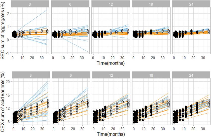
In Fig. 6 a comparison of kinetic modelling and linear extrapolation is shown for analysis of multiple (23)
batches of rituximab, showing predicted curves (i.e. not prediction intervals as in Fig. 5) of sum of aggregates
(Fig. 6, upper panels) and sum of acidic variants (Fig. 6, lower panels). Clearly, the kinetic model is able to more
accurately predict the actual changes in the quality attributes. Especially when using only short-term data for
model building linear extrapolation overestimates the actual variability of the system, while kinetic model-based
predictions are accurate and do not vary between batches already when using 3 month data only. To sum up,
result comparison of prediction intervals for a single batch (Fig. 5) together with result comparison of prediction
curves for multiple batches provides a clear conclusions that kinetic modelling can more accurately predict the
assessed stability quality attributes than linear extrapolation.
Approaching rapid stability prediction by exploiting a month‑long stability study at tempera‑
tures beyond traditional stress conditions. Higher temperatures lead to faster kinetics of degrada-
tion processes. This fundamental knowledge of chemistry could potentially be used for accelerating stability
prediction even further. Two limitations, arising from the nature of the observed degradation, for using kinetic
modelling can potentially affect such rapid screening: (i) the temperature up to which the simple kinetic model
can sufficiently/successfully describe observed changes and (ii) the variability of the experimental data, which
sets the minimal time interval in which data has to be collected for the model to give sufficiently robust fit. As
discussed in Fig. 4, some stability quality attributes follow the same mechanisms at temperatures above 40 °C as
at intendent storage conditions (5 °C) and in these cases degradation can be successfully described by (appar-
ent) first order degradation kinetic model across whole temperature range. For presented charge variant studies,
acceptable maximum storage temperature could be as high as 60 °C, for fragmentation 55 °C, etc. However,
acceptable temperature ranges depend on the molecule and should be assessed on a case-by-case basis.
Scientific Reports | (2021) 11:20534 | https://doi.org/10.1038/s41598-021-99875-9 10
Vol:.(1234567890)www.nature.com/scientificreports/
Figure 6. Comparison of kinetic modelling (orange) and linear (blue) extrapolation, showing prediction curves
based on 3, 6, 12, 18 or 24 month experimental stability data (black data points). In grey, remaining measured
data points at intended storage are shown for visual verification of the prediction intervals. Data shown is for
23 rituximab batches stored at 5 °C. For kinetic modelling data points from 25 and 40 °C conditions up to the
respective time point were used (data points not shown for clarity reasons).
To achieve accurate and narrow prediction intervals in the shortest possible time, we generally obtain stability
data from three or more temperature conditions, which are up to the temperature at which kinetic mechanism
changes and the simple kinetic model cannot describe the observed change. How to identify this maximal tem-
perature has been discussed above (under the Fig. 4). Here we assessed accuracy and precision of the prediction.
Rapid stability prediction exploiting data from a 4-week-long stability study including temperatures above 40 °C
is shown in Fig. 7. In order to demonstrate rapid stability prediction we tried to model stability profiles only
based on two weeks data. In case reliable model could not be achieved (R2 < 0.9, prediction intervals were not
verified by measurements or 36 months prediction intervals are wider as generic specifications described above
(Table 2)) then additional time points were included until model reliability was reached. That leads to different
number of data points per quality attribute shown on Fig. 7 (top panel). The minimal stability study time interval
needed to achieve required prediction interval widths48 were thus two weeks for sum of acidic variants, three
weeks for amount of main variant and four weeks for fragmentation and aggregation (Fig. 7). We speculate that
by optimising the study design further we could achieve the same precision of predictions even faster for some
quality attributes. For example, first data point for fragmentation at 40 and 25 °C is at 1 month. If data for first
and second week time points would be available for these two temperatures, we could probably calculate the
prediction interval for mAb1 molecule already after two weeks instead of four weeks as shown on Fig. 7c. Since
model predicted increase in fragmentation at two week time point is 0.4% and 1.2% for 25 and 40 °C, respectively,
which is above method variability of 0.2%, data from at least 3 temperatures with measurable degradation would
be available. This is, as already discussed, enough for a reliable prediction.
Discussion
Kinetic modelling for predicting long-term stability from accelerated stability data was evaluated for several
monoclonal antibodies belonging to IgG1, IgG2 families/types and a fusion protein. Presented results suggest
that by applying a degradation model-based on first order kinetics and the Arrhenius equation on accelerated
stability data, we can predict long-term (up to 3 year) changes of most relevant stability indicating quality
attributes in solution. The highly successful in prediction (above 90% accuracy for 4 different protein molecules)
quality attributes include fragments, chemical modifications (acidic variants and main peak), purity, aggregates
and potency. Low accuracy is obtained for prediction of basic variants. The reason lies in use of simple first
order kinetic model, which cannot cover possible non-monotonic variability of basic variants in time (Fig-
ure S4). A cause for more complex kinetic mechanism of basic variants change over time arises possibly from
Scientific Reports | (2021) 11:20534 | https://doi.org/10.1038/s41598-021-99875-9 11
Vol.:(0123456789)www.nature.com/scientificreports/
Figure 7. Rapid stability prediction for mAb1 molecule from stability data at temperatures 25 to 60 °C. (a)
Two weeks data for acidic variants, (b) three weeks for main variants, both measured by CEX, (c) four weeks
for fragmentation measured by nrCE-SDS and (d) four weeks for sum of aggregates by SEC. Highly accelerated
experimental stability data (data points) and model fits (full lines) are shown in the upper panels, to generate
prediction curves (full line) and prediction intervals (dashed lines) with measured data (solid circles) in the
bottom panels. Note that different temperature intervals had to be used for different stability quality attributes,
depending on the nature of degradation process kinetics. Measured value at t = 0 is designated by a black solid
circle.
the temperature/pH dependence of succinimide formation49.First order kinetic model would fail to describe any
non-monotonic changes of any quality attribute. Low prediction accuracy is also obtained for subvisible particles
(data not shown), mainly due to high variability of available analytical methods and high complexity of parti-
cle formation mechanisms50–53 which do not follow Arrhenius kinetics. From a biopharmaceutical application
perspective, none of the both quality attributes show any trend at intended storage temperature for investigated
molecules and are therefore not shelf-life limiting. For other quality attributes the predictions were successfully
determined by using up to 6 month stability data containing three or more temperature conditions (usually
5 °C, 25 °C and 40 °C). The verification of long-term stability predictions at the intended storage temperature
of 5 °C was evaluated by comparison of the 95% probability prediction interval and experimental data obtained
during the long-term stability studies lasting up to 36 months. Results are summarised in Table 1 for 4 different
molecules (mAb1, rituximab, adalimumab and etanercept). Percentage of experimental stability data between 6
and 36 months at 5 °C that are within the 95% probability prediction interval is above 90% for all model fits with
goodness of fit R2 ≥ 0.9. Robustness of the model stability prediction is additionally supported by applying the
kinetic modelling to combinations of stability data subsets, which included different temperatures, and analysing
the goodness of fit and model parameters. If values for model parameters do not vary between different stability
data subsets, this is a strong indication for the appropriateness of the kinetic model and the overall accuracy
and robustness of the prediction approach (Fig. 4). Furthermore, by fitting the model with data subsets we can
estimate the maximal temperature up to which molecule degradation follows Arrhenius behaviour. The most
prominent advantage of using the identified highest temperature storage condition is faster molecule degradation,
which allows to conduct a shorter accelerated stability study, which based on our results does not compromise
accuracy or robustness of model prediction (Fig. 7). However, to evaluate the associated risk and benefits of very
short (weeks) accelerated stability studies, additional research still needs to be done.
Aggregation is a common stability-limiting factor for biologics. It is also known that aggregation is a com-
plex process that in general embraces several aggregation pathways, which are temperature-dependent9,50. For
mAbs Wang and R oberts3 confirmed Arrhenius behaviour in a temperature range from 5 to 40 °C, at higher
temperatures the linearity of Arrhenius plot vanished. These findings are in agreement with our data shown on
Fig. 4 (panels f, g and h), where at temperatures above 40 °C we found an increase of fitted value for Ea for all
three molecules studied indicating a change in aggregation process. The importance of limiting the temperature
range for kinetic modelling of aggregation is demonstrated in Figure S5. Obtained aggregation rates based on
up to 40 °C stability data are in a range of 0.1 to 0.2% increase per year and are in agreement with experimental
observations. While adding 45 °C data to the modelling dataset results in 100 times slower predicted aggregation
rate (Figure S5c). According to the literature, there are notable evidences that aggregation pathways are connected
with the conformational stability54,55. Our aggregation results (Fig. 4, panels f and g) indeed briefly indicate
that the aggregation pathway changes with increasing temperature, which might be linked to the mentioned
temperature-induced change in conformational stability. Nevertheless, the presented approach for identification
Scientific Reports | (2021) 11:20534 | https://doi.org/10.1038/s41598-021-99875-9 12
Vol:.(1234567890)You can also read