Emissions of methane in Europe inferred by total column measurements
←
→
Page content transcription
If your browser does not render page correctly, please read the page content below
Atmos. Chem. Phys., 19, 3963–3980, 2019
https://doi.org/10.5194/acp-19-3963-2019
© Author(s) 2019. This work is distributed under
the Creative Commons Attribution 4.0 License.

Emissions of methane in Europe inferred by
total column measurements
Debra Wunch1 , Dylan B. A. Jones1 , Geoffrey C. Toon2 , Nicholas M. Deutscher3,4 , Frank Hase5 , Justus Notholt4 ,
Ralf Sussmann6 , Thorsten Warneke4 , Jeroen Kuenen7 , Hugo Denier van der Gon7 , Jenny A. Fisher3 , and
Joannes D. Maasakkers8
1 Department    of Physics, University of Toronto, Toronto, Ontario, Canada
2 Jet Propulsion Laboratory, California Institute of Technology, Pasadena, California, USA
3 Centre for Atmospheric Chemistry, University of Wollongong, Wollongong, New South Wales, Australia
4 Institute of Environmental Physics, University of Bremen, Germany
5 Karlsruhe Institute of Technology, IMK-ASF, Karlsruhe, Germany
6 Karlsruhe Institute of Technology, IMK-IFU, Garmisch-Partenkirchen, Germany
7 TNO Dept Climate, Air and Sustainability, Utrecht, the Netherlands
8 School of Engineering and Applied Sciences, Harvard University, Cambridge, Massachusetts, USA

Correspondence: Debra Wunch (dwunch@atmosp.physics.utoronto.ca)

Received: 12 March 2018 – Discussion started: 7 May 2018
Revised: 15 March 2019 – Accepted: 17 March 2019 – Published: 28 March 2019

Abstract. Using five long-running ground-based atmo-            FCCC, 2015; Kona et al., 2016). This, in turn, has motivated
spheric observatories in Europe, we demonstrate the utility     countries to seek methods of reducing their greenhouse gas
of long-term, stationary, ground-based measurements of at-      emissions. In Europe, methane emissions account for a sig-
mospheric total columns for verifying annual methane emis-      nificant fraction (about 11 % by mass of CO2 equivalent) of
sion inventories. Our results indicate that the methane emis-   the total greenhouse gas emissions (UNFCCC, 2017). The
sions for the region in Europe between Orléans, Bremen, Bi-     lifetime of atmospheric methane is significantly shorter than
ałystok, and Garmisch-Partenkirchen are overestimated by        for carbon dioxide, its 100-year global warming potential is
the state-of-the-art inventories of the Emissions Database      significantly larger, and it is at near steady state in the at-
for Global Atmospheric Research (EDGAR) v4.2 FT2010             mosphere; therefore, significant reductions in methane emis-
and the high-resolution emissions database developed by the     sions are an effective short-term strategy for reducing green-
Netherlands Organisation for Applied Scientific Research        house gas emissions (Dlugokencky et al., 2011). Emission re-
(TNO) as part of the Monitoring Atmospheric Composition         duction strategies that include both methane emission reduc-
and Climate project (TNO-MACC_III), possibly due to the         tions and carbon dioxide reductions are thought to be among
disaggregation of emissions onto a spatial grid. Uncertain-     the most effective at slowing the increase in global tempera-
ties in the carbon monoxide inventories used to compute the     tures (Shoemaker et al., 2013). Thus, it is important to know
methane emissions contribute to the discrepancy between our     exactly how much methane is being emitted and the geo-
inferred emissions and those from the inventories.              graphic and temporal source of the emissions. This requires
                                                                an approach that combines state-of-the-art emissions inven-
                                                                tories that contain information about the specific point and
                                                                area sources of the known emissions and timely and long-
1   Introduction                                                term measurements of greenhouse gases in the atmosphere
                                                                to verify that the emissions reduction targets are met.
Recent global policy agreements have led to renewed efforts        Because atmospheric methane is well-mixed and has a
to reduce greenhouse gas emissions to cap global tempera-       lifetime of about 12 years (Stocker et al., 2013), it is trans-
ture rise (e.g., Conference of the Parties 21, COP 21; UN-

Published by Copernicus Publications on behalf of the European Geosciences Union.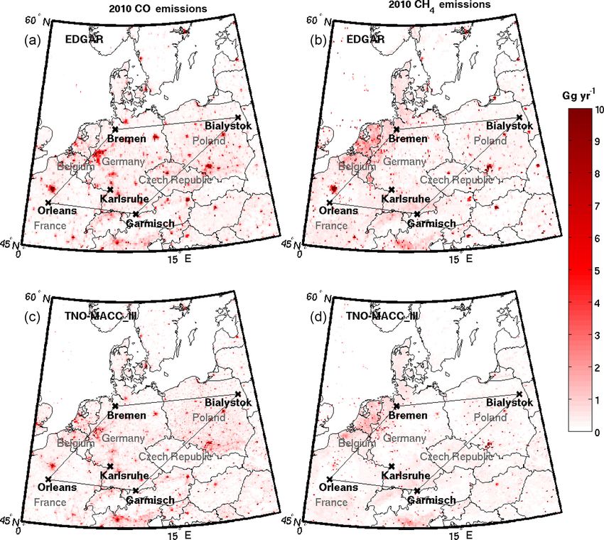
3964                                                                    D. Wunch et al.: TCCON-derived European methane

ported far from its emission source, making source attri-           tempted to extract regional methane emission information
bution efforts challenging from atmospheric measurements            from these existing ground-based remote sensing observato-
alone. Atmospheric measurements are often assimilated into          ries.
“flux inversion” models to locate the sources of the emis-             In this paper, we will describe our methods for computing
sions (e.g., Houweling et al., 2014) but rely on model wind         the emissions of methane using five stationary ground-based
fields to drive transport, and they also tend to have spatial       remote sensing instruments located in Europe in Sect. 2. Our
resolutions that do not resolve subregional scales. Methane         results and comparisons to the state-of-the-art inventories are
measurement schemes that constrain emissions on local and           shown in Sect. 3, and we summarize our results in Sect. 4.
regional scales are thus important to help identify the sources
of the emissions and to verify inventory analyses. Regional-
or national-scale emissions are important to public policy as       2   Methods
those emissions are reported annually to the United Nations
                                                                    Our study area is the region between five long-running atmo-
Framework Convention on Climate Change (UNFCCC).
                                                                    spheric observatories situated in Europe. Three of the stations
   The atmospheric measurement techniques that are used to
                                                                    are in Germany: Bremen (Notholt et al., 2014), Karlsruhe
estimate methane emissions include measurements made in
                                                                    (Hase et al., 2014), and Garmisch-Partenkirchen (Sussmann
situ, either on the ground, from tall towers, or from aircraft.
                                                                    and Rettinger, 2014). The other two are in Poland (Białys-
Remote sensing techniques are also used, either from space
                                                                    tok, Deutscher et al., 2017) and France (Orléans, Warneke
or from the ground. The spatial scale of the sensitivity to
                                                                    et al., 2014). Each station measures the vertical column-
emissions differs with the measurement technique: surface in
                                                                    averaged dry-air mole fraction of carbon dioxide (XCO2 ),
situ measurements provide information about local emissions
                                                                    carbon monoxide (XCO ), methane (XCH4 ), and other trace
on urban scales (e.g., McKain et al., 2015; Hopkins et al.,
                                                                    gas species. The locations are shown in Fig. 1, overlaid on
2016), and aircraft in situ measurements can provide infor-
                                                                    a nighttime light image from the National Aeronautics and
mation about regional- and synoptic-scale fluxes (e.g., Jacob
                                                                    Space Administration (NASA) to provide a sense of the pop-
et al., 2003; Kort et al., 2008, 2010; Wofsy, 2011; Baker
                                                                    ulation density of the area. These observatories are part of the
et al., 2012; Frankenberg et al., 2016; Karion et al., 2016).
                                                                    Total Carbon Column Observing Network (TCCON, Wunch
Satellite remote sensing techniques provide information use-
                                                                    et al., 2011) and have been tied to the World Meteorological
ful for extracting emission information on larger scales (re-
                                                                    Organization trace-gas scale through comparisons with verti-
gional to global) (e.g., Silva et al., 2013; Schneising et al.,
                                                                    cally integrated, calibrated in situ profiles over the observato-
2014; Alexe et al., 2015; Turner et al., 2015) and for large
                                                                    ries (Wunch et al., 2010; Wunch et al., 2015; Messerschmidt
point or urban sources (e.g., Kort et al., 2012, 2014; Nas-
                                                                    et al., 2011; Geibel et al., 2012).
sar et al., 2017). Several studies have shown the importance
                                                                       Following a similar method to Wunch et al. (2009, 2016),
of simultaneous measurements of co-emitted species (e.g.,
                                                                    we estimate emissions of methane from the data recorded
C2 H6 and CH4 or CO and CO2 , Aydin et al., 2011; Simpson
                                                                    from the TCCON observatories, coupled with gridded inven-
et al., 2012; Peischl et al., 2013; Silva et al., 2013; Haus-
                                                                    tories of carbon monoxide within the region. We compute
mann et al., 2016; Wunch et al., 2016; Jeong et al., 2017)
                                                                    changes (or “anomalies”) in XCH4 and XCO that we will re-
or co-located measurements (e.g., Wunch et al., 2009, 2016),
                                                                    fer to as 1XCH4 and 1XCO , and we then compute the slopes
showing the added analytical power of the combination of
                                                                    relating 1XCH4 to 1XCO . From the computed slopes (α), we
atmospheric tracer information. Ground-based remote sens-
                                                                    can infer emissions of methane (ECH4 ) if emissions of carbon
ing instruments have been used to estimate methane emis-
                                                                    monoxide (ECO , in mass per unit time) are known, using the
sions on urban (e.g., Wunch et al., 2009; Hase et al., 2015;
                                                                    following relationship:
Wunch et al., 2016) and sub-urban (e.g., Chen et al., 2016;
Viatte et al., 2017) scales. In Hase et al. (2015), Viatte et al.              mCH4
                                                                    ECH4 = α        ECO ,                                        (1)
(2017), and Chen et al. (2016), the authors have placed                        mCO
mobile ground-based remote sensing instruments around a
                                                                           mCH
particular emitter of interest (e.g., a city, dairy, or neigh-      where mCO4 is the ratio of the molecular masses of CH4 and
borhood) and have designed short-term campaigns to mea-             CO.
sure the difference between upwind and downwind atmo-                  In Wunch et al. (2009, 2016), measurements from a sin-
spheric methane abundances. From these differences the au-          gle atmospheric observatory were used to infer emissions
thors have computed emission fluxes. However, there is a net-       because the unique dynamics of the region advected the pol-
work of nonmobile ground-based remote sensing instruments           luted air mass into and out of the study area diurnally. In this
that have been collecting long-term measurements of atmo-           paper, we rely on several stations to provide measurements
spheric greenhouse gas abundances. These instruments were           of the boundary of the study region to measure CO and CH4
not placed intentionally around an emitter of interest, but         emitted between the stations. This analysis relies on a few
collectively they ought to contain information about nearby         assumptions about the nature of the emissions. First, that the
emissions. To date, there have been no studies that have at-        lifetimes of the gases of interest are longer than the transport

Atmos. Chem. Phys., 19, 3963–3980, 2019                                              www.atmos-chem-phys.net/19/3963/2019/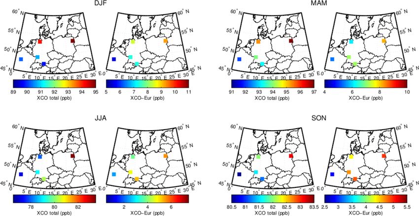
D. Wunch et al.: TCCON-derived European methane                                                                                   3965

Figure 1. The locations of the TCCON observatories overlaid on a NASA nighttime light image. From west to east, the stations are Orléans
(or, pink), Karlsruhe (ka, green), Bremen (br, blue-green), Garmisch-Partenkirchen (gm, orange), and Białystok (bi, purple).

time within the region. This is the case both for methane,            surface layer column averaging kernel value, as we assume
which has an atmospheric lifetime of 12 years, and for car-           that the anomalies are due to emissions near the surface. The
bon monoxide, which has an atmospheric lifetime of a few              slopes computed for each year and each pair of stations are
weeks. Second, we assume that typical emissions are consis-           shown in Fig. 2.
tent over time periods longer than a few days so that they are           The farthest distance between the European TCCON sta-
advected together. The nature of the emissions in this region         tions included in this study is between Orléans and Białys-
(mostly residential and industrial energy needs) supports this        tok (1580 km). Climatological annual mean surface wind
assumption. Third, we assume that the spatial distribution of         speeds from the National Centers for Environmental Pre-
the emissions is similar for CH4 and CO, as confirmed by              diction (NCEP) and National Center for Atmospheric Re-
the inventory maps (Fig. A3). This method does not require            search (NCAR) reanalysis (Kalnay et al., 1996) within the
carbon monoxide and methane to be co-emitted (as they gen-            study area are about 6 km h−1 (Fig. A1). The air from Or-
erally do not have the same emissions sources).                       léans will quickly mix vertically from the surface where
   To compute anomalies and slopes, we first filter the data          the winds aloft are more rapid than at the surface (see Ap-
to minimize the impact of data sparsity and air mass differ-          pendix B). Thus, air from Orléans would normally reach Bi-
ences between stations (Appendix A). Then, for each sta-              ałystok in a few days. To determine whether these anoma-
tion, the daily median value is subtracted from each mea-             lies are consistent throughout the transport time through the
surement. This reduces the impact of the station altitude and         study area, we compute anomalies between sites lagged by
any background seasonal cycle from aliasing into the results.         up to 14 days. The slopes of the anomalies do not change sig-
Subsequently, we compute the differences in the XCH4 and              nificantly or systematically with the lag time (Appendix B;
XCO abundances measured at the same solar zenith and so-              Fig. A2), presumably because the atmospheric composition
lar azimuth angles on the same day at two TCCON stations.             within the study area is relatively well-mixed or because the
By computing anomalies at the same solar zenith angles, we            emissions are relatively consistent from day to day within the
minimize any impact that air-mass-dependent biases could              study area.
have on the calculated anomalies. This analysis is repeated              Previous papers have used carbon dioxide instead of car-
for all combinations of pairs of stations within the study area.      bon monoxide to infer methane emissions. We choose to
The vertical sensitivity of the TCCON measurements is ex-             compute emissions using measurements of XCO instead of
plicitly taken into account by dividing the anomalies by the          XCO2 in this work because the natural CO2 fluxes in the re-

www.atmos-chem-phys.net/19/3963/2019/                                                   Atmos. Chem. Phys., 19, 3963–3980, 2019
3966                                                                            D. Wunch et al.: TCCON-derived European methane

Figure 2. The bars show the methane to carbon monoxide anomaly slopes for each site pair. The method of computing these anomaly slopes
is detailed in Sect. 2 of the main text. The black targets indicate the median value of the slope for that year, when all site pairs are considered
simultaneously, and the 25th and 75th quartiles of the median value are indicated by the vertical black bars. Outliers are indicated by open
black circles.

gion are large compared with the anthropogenic emissions,                   (TNO-MACC_III). The EDGAR version v4.3.1_v2 of Jan-
and they have a strong diurnal and seasonal cycle. The dis-                 uary 2016 annual gridded inventory is available at 0.1◦ ×0.1◦
tance between the stations is large enough that local (sub-                 spatial resolution and reports global emissions from the year
daily) uptake of CO2 differs from station to station, signifi-              2000 to 2010 (Olivier et al., 1994; EC-JRC and PBL, 2016).
cantly obscuring the relationships between methane and car-                 The TNO-MACC_III inventory is a Europe-specific air qual-
bon dioxide, and thus the anomaly slopes, especially in the                 ity emissions inventory, available on a 0.125◦ ×0.0625◦ grid,
summer months. While the emissions inventory of anthro-                     and reports emissions for 2000–2011 (Kuenen et al., 2014).
pogenic CO2 may be more accurate than the CO inventory in                   Both EDGAR and TNO-MACC_III provide spatially and
the region, the presence of these large natural fluxes of CO2               temporally coincident methane inventories which we use to
precludes its use in the anomaly slope calculation. The accu-               compare with our inferred emissions. We use the EDGAR
racy of our method, therefore, is limited by the accuracy of                version v4.2 FT2010 and the TNO-MACC_III methane in-
the carbon monoxide emission inventory. Fires could provide                 ventories.
a large flux of CO without a large CH4 flux, and this should                   Using country-level emissions reported through 2015 from
also be taken into consideration in these types of analyses. In             the European Environment Agency (EEA, 2015), we extrap-
our study area fluxes from fires are small.                                 olate the EDGAR and TNO-MACC_III gridded inventory
                                                                            CO emissions for the study area through 2015. This facil-
2.1    Inventories                                                          itates more direct comparisons with the TCCON measure-
                                                                            ments, which begin with sufficient data for our study in 2009.
To obtain an estimate of carbon monoxide emissions (ECO )                   We extrapolate the emissions by scaling the total emissions
within the study area, we use gridded inventories and sum                   from the countries that are intersected by the area of interest
the emissions within the study area to compare with our                     (Germany, Poland, Belgium, France, Luxembourg, and the
emissions inferred from the TCCON measurements (see                         Czech Republic) to the last reported year of emissions from
Appendix C and Fig. A3 for details). The two invento-                       the inventory. We then assume that the same scaling factor
ries employed here are the Emissions Database for Global                    applies for each subsequent year. The details of the extrapo-
Atmospheric Research (EDGAR) and the Netherlands Or-                        lation method are in Appendix D and Figs. A4 and A5.
ganisation for Applied Scientific Research (TNO) high-                         The time series of the reported emissions from 2000
resolution emissions database developed as part of the                      to 2015 are shown in Fig. 3. The inventories and scaled
Monitoring Atmospheric Composition and Climate project

Atmos. Chem. Phys., 19, 3963–3980, 2019                                                        www.atmos-chem-phys.net/19/3963/2019/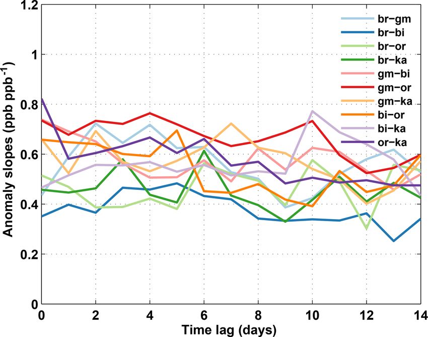
D. Wunch et al.: TCCON-derived European methane                                                                               3967

                                                                      gional CH4 emissions (e.g., Wunch et al., 2009; Wecht et al.,
                                                                      2014) but to underestimate oil and gas emissions (e.g., Miller
                                                                      et al., 2013; Buchwitz et al., 2017). However, recent methane
                                                                      isotope analysis by Röckmann et al. (2016) has suggested
                                                                      that the EDGAR inventory overestimates fossil-fuel-related
                                                                      emissions. The study area of interest here has little oil and
                                                                      gas production, except for some test sites in Poland (USEIA,
                                                                      2015), no commercial shale gas industry, and few pipelines.

                                                                      2.2   Model experiment

                                                                      To test whether the anomaly method described in Sect. 2
                                                                      can accurately infer methane emissions, we conducted a
                                                                      modeling experiment using version v12.1.0 of the GEOS-
                                                                      Chem model (http://www.geos-chem.org, last access: 4 Jan-
                                                                      uary 2019) to simulate methane and carbon monoxide for
Figure 3. This figure shows the summed EDGAR (green) and              the year 2010. The model is driven by the Modern-Era Ret-
TNO-MACC_III (orange) emissions within the study area for CO          rospective analysis for Research and Applications, version 2
(squares) and CH4 (triangles). The study area is defined in Fig. 1.
                                                                      (MERRA-2) meteorology from the NASA Global Modeling
All emissions are shown in units of Tg yr−1 . Extrapolation begins
after 2010 for EDGAR and 2011 for TNO-MACC_III.
                                                                      and Assimilation Office. The native resolution of the mete-
                                                                      orological fields is 0.25◦ × 0.3125◦ , with 72 vertical levels
                                                                      from the surface to 0.01 hPa, which we degraded to 2◦ × 2.5◦
                                                                      and 47 vertical levels. We use the linear CO-only and CH4 -
country-level reported emissions for this region suggest that         only simulations of GEOS-Chem, with prescribed monthly
emissions of CO and CH4 have decreased by about 40 %                  mean OH fields. In the CO-only simulation, global anthro-
and 20 %, respectively, between 2000 and 2015. The TNO-               pogenic emissions are from EDGAR v4.3.1, which are over-
MACC_III carbon monoxide emissions are on average 15 %                written regionally with the following emissions: the Cooper-
higher than the EDGAR v.4.3.1 emissions in the study area.            ative Programme for Monitoring and Evaluation of the Long-
The total TNO-MACC_III and EDGAR methane emissions                    range Transmission of Air Pollutants in Europe (EMEP), the
agree to within 2 % in the study area.                                U.S. Environmental Protection Agency National Emission
   An earlier version of the EDGAR carbon monoxide in-                Inventory for 2011 (NEI2011), the MIX inventory for Asia,
ventory was evaluated by Stavrakou and Müller (2006)                  the Visibility Observational (BRAVO) Study Emissions In-
and Fortems-Cheiney et al. (2009), who assimilated satel-             ventory for Mexico, and the criteria air contaminants (CAC)
lite measurements of CO using the EDGAR v3.3FT2000                    inventory for Canada. The sources of CO from the oxida-
CO emissions inventory as the a priori. Stavrakou and                 tion of CH4 and volatile organic compounds (VOCs) are pre-
Müller (2006) found that, over Europe, the a posteriori emis-         scribed following Fisher et al. (2017). For the CH4 -only sim-
sions increase by less than 15 % when assimilating carbon             ulation, the emissions are as described in Maasakkers et al.
monoxide from the Measurements of Pollution in the Tropo-             (2019). Global anthropogenic emissions are from EDGAR
sphere (MOPITT) satellite instrument (Emmons et al., 2004).           v4.3.2, but the US emissions were replaced with those from
Fortems-Cheiney et al. (2009) assimilated Infrared Atmo-              Maasakkers et al. (2016), and emissions from wetlands are
spheric Sounding Interferometer (IASI) CO (Clerbaux et al.,           from WetCHARTs version 1.0 (Bloom et al., 2017). For both
2009) and MOPITT CO and found that the a posteriori emis-             CO and CH4 simulations, emissions from biomass burning
sions increase by 16 % and 45 %, respectively.                        are from the Quick Fire Emissions Dataset (QFED) (Dar-
   The more recent EDGAR v4.3.1 CO emissions in our                   menov and Silva, 2015). The biomass burning in the study
study are 24 % lower than the EDGAR v3.3FT2000 CO                     area produces less than 2 % of the total anthropogenic emis-
emissions for the year 2000, so it may be that the EDGAR              sions of CO.
v4.3.1 CO emissions are significantly underestimated. How-               We used identical OH fields (from version v7-02-03 of
ever, assimilations of CO are known to be very sensitive              GEOS-Chem) for the CO and CH4 simulations, so that the
to the chemistry described in the model: most notably the             chemical losses of methane and carbon monoxide are consis-
OH chemistry (Protonotariou et al., 2010; Yin et al., 2015).          tent, and ran tagged CO experiments so that we could iden-
Therefore, it is difficult to determine how much of the dis-          tify the source of the emissions. The model atmospheric car-
crepancy between versions of the model is from the inventory          bon monoxide and methane profiles were integrated to com-
or the model chemistry.                                               pute simulated XCO and XCH4 . To illustrate the sensitivity
   The EDGAR methane inventory has been evaluated in sev-             of the modeled fields to European emissions, we show the
eral previous studies. It has been shown to overestimate re-          seasonal means of the modeled XCO sampled at the five TC-

www.atmos-chem-phys.net/19/3963/2019/                                                 Atmos. Chem. Phys., 19, 3963–3980, 2019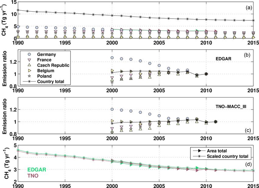
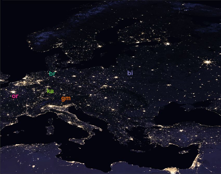
3968                                                                      D. Wunch et al.: TCCON-derived European methane

Figure 4. This figure compares seasonally averaged modeled total XCO with the XCO contribution from emissions in Europe. Each season
has two maps: the left map shows the total XCO and the right map shows the contribution from European emissions (XCO−Eur ). The spatial
pattern of the gradients in modeled XCO between the TCCON stations is reflected in the European contribution.

CON stations in Fig. 4. Also plotted is the column contribu-             While the inferred annual emissions agree well with the
tion (XCO−Eur ) from CO emissions only in Europe (defined             modeled annual emissions, the seasonal pattern of the emis-
as the broader region between 0–45◦ E and 45–55◦ N). As               sions inferred from the anomaly analysis differs from that of
can be seen, the spatial pattern of the differences in modeled        the model. The anomaly analysis overestimates emissions in
XCO between the TCCON stations is reflected in XCO−Eur .              the winter and underestimates emissions in the summer. This
We calculated the anomalies in XCO and XCO−Eur , using                may be due to small spatial inhomogeneities in the column
the same approach employed with the atmospheric data, and             enhancements from VOC (biogenic) emissions that influence
found that the anomalies in XCO−Eur , which represent the             the anomaly analysis most in summertime when VOC emis-
direct influence of European emissions on atmospheric CO,             sions are largest. Including the VOC emissions in the total
account for about 35 % of the anomalies in XCO . This con-            carbon monoxide emissions leads us to infer annual methane
firms that the XCO anomalies between the TCCON stations               emissions that are overestimated by 15 %, increasing the in-
are sensitive to European emissions.                                  ferred summertime emissions without significantly changing
   To estimate the modeled CH4 emissions using the mod-               the inferred wintertime emissions.
eled CO, the modeled XCO and XCH4 were interpolated to the               The seasonal analysis suggests that the 2 % agreement in
locations of the TCCON stations and anomalies and slopes              the annual emission estimate may reflect the compensating
were computed. We then applied Eq. (1) to our anomaly                 effects of discrepancies over the seasonal cycle, and improv-
slopes to compute methane emissions from the known CO                 ing the seasonal estimate may require a better treatment of
emissions, accounting for only the CO emissions from an-              the VOC contribution to atmospheric CO. Nevertheless, the
thropogenic, biomass burning, and biofuel sources. We ne-             results here suggest that for this region of Europe, where
glect sources of CO emissions from the oxidation of CH4               VOC and methane oxidation emissions lead to relatively
and VOCs because the column enhancements for those emis-              spatially uniform column enhancements and fire emissions
sions are relatively spatially uniform across this region of Eu-      are small, we can successfully use the anomaly method de-
rope, and thus they should not contribute significantly to the        scribed in Sect. 2 to infer annual methane emissions.
anomalies. The resulting annual CH4 emissions agree well
with the model emissions: the inferred emissions from the
anomaly analysis are higher than the model emissions by less
than 2 % (Fig. 5).

Atmos. Chem. Phys., 19, 3963–3980, 2019                                                 www.atmos-chem-phys.net/19/3963/2019/
D. Wunch et al.: TCCON-derived European methane                                                                                    3969

Figure 5. This figure shows the results from the modeling experiment using GEOS-Chem. Panel (a) shows the model 1XCH4 –1XCO slopes
for each month and pair of stations (indicated by the colors). The median slopes for each month are overlaid with grey squares. Panel (b)
shows the model carbon monoxide emissions (excluding VOC and methane oxidation) and the model methane emissions. The inferred
methane emissions from our tracer–tracer slope method are plotted in pink squares. Panel (c) shows the annual methane emissions from the
tracer–tracer slope method and the model.

                                                                       3   Results and discussion

                                                                       To compute methane emissions, we apply Eq. (1) to our
                                                                       anomaly slopes and the inventory-reported carbon monox-
                                                                       ide emissions in the study region (Fig. 6). If we choose the
                                                                       mean of the reported CO emissions from EDGAR v4.3.1
                                                                       and TNO-MACC_III, the methane emissions we compute
                                                                       within the study area based on the TCCON measurements
                                                                       are 1.7 ± 0.3 Tg yr−1 in 2009, with a non-monotonic de-
                                                                       crease to 1.2 ± 0.3 Tg yr−1 in 2015. The uncertainties quoted
                                                                       here are from the standard errors on the data slope fitting
                                                                       only; we have not included uncertainties from the invento-
                                                                       ries. The magnitude of methane emissions we compute from
                                                                       the TCCON data are, on average, about 2.3 times lower
                                                                       than the methane emissions reported by EDGAR and about
Figure 6. The black line is the summed EDGAR (green) and TNO-          2 times lower than the methane emissions reported by TNO-
MACC_III (orange) methane emissions within the study area shown
                                                                       MACC_III.
in Fig. 1. The grey lines indicate the projected emissions based on
                                                                          Our method of inferring methane emissions depends criti-
scaling the country-level emissions reported by the UNFCCC (UN-
FCCC, 2017) to the area emissions in 2010 for EDGAR and 2011           cally on the carbon monoxide inventory. The carbon monox-
for TNO-MACC_III. The lower solid lines show the emissions in-         ide emissions for 2010 in the study area from our GEOS-
ferred from the TCCON anomaly analysis using CO emissions from         Chem model run, derived from EMEP emissions, were
the two models, and the dashed lines indicate the 5th and 95th per-    6.4 Tg, about 35 % higher than the average of the EDGAR
centiles.                                                              and TNO-MACC_III emissions for that year. This magni-
                                                                       tude underestimate has also been suggested by Stavrakou and
                                                                       Müller (2006) and Fortems-Cheiney et al. (2009) using in-
                                                                       dependent data. Using the GEOS-Chem carbon monoxide

www.atmos-chem-phys.net/19/3963/2019/                                                    Atmos. Chem. Phys., 19, 3963–3980, 2019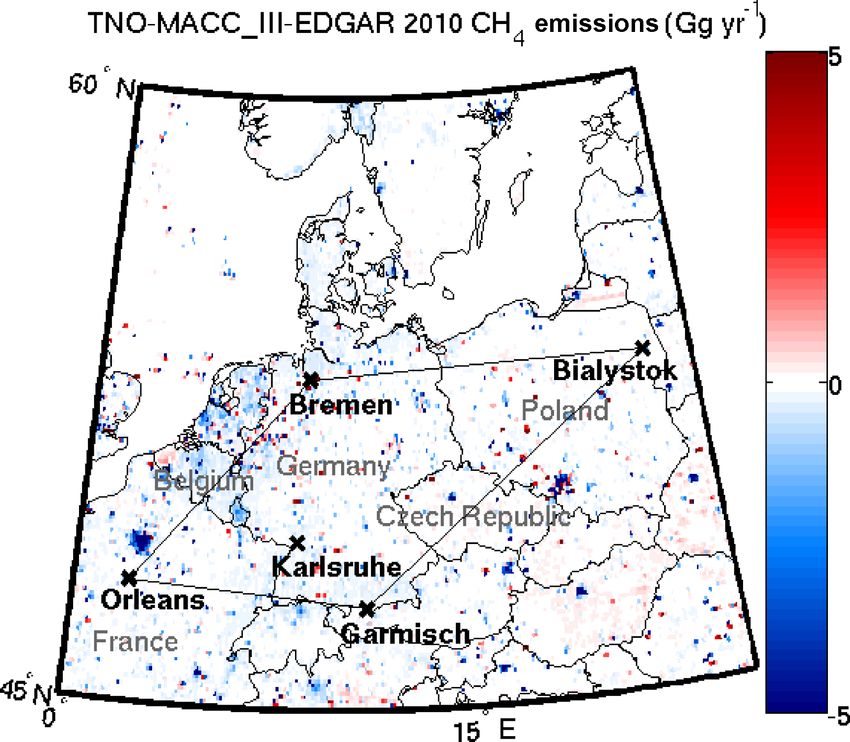
3970 D. Wunch et al.: TCCON-derived European methane
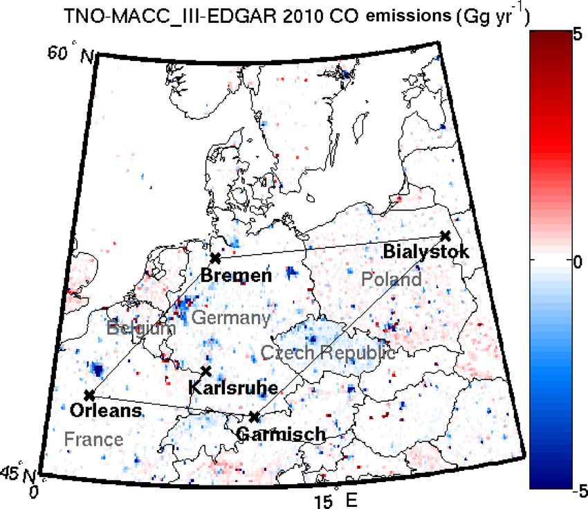
Figure 7. This map shows the difference between the TNO- Figure 8. This map shows the difference between the TNO-
MACC_III carbon monoxide emissions and the EDGAR emissions MACC_III methane emissions and the EDGAR emissions for the
for the year 2010. The black straight lines delineate the study year 2010. The labeling and coloring follows that in Fig. 7.
area from the surrounding region. The TCCON stations included
in this study are marked with black “x” symbols and labeled in
black bold font. The countries intersected by or contained within
the study area are labeled in grey. Warm (red) colors indicate that
the TNO-MACC_III inventory is larger than the EDGAR inventory; In contrast to the carbon monoxide spatial distribution, the
cool (blue) colors indicate that the EDGAR inventory is larger than TNO-MACC_III methane emissions are generally smaller
TNO-MACC_III. everywhere, except for discrete point sources.
Comparing country-level carbon monoxide emissions re-
ported in 2010 with the inventories shows reasonable agree-
emissions increases the methane emissions inferred by the ment, which is expected since the inventories use country-
anomaly analysis to 2.4 ± 0.3 Tg in 2010. This value remains level reports as input. The sum of the carbon monoxide emis-
lower than the EDGAR and TNO-MACC_III methane emis- sions within the entire countries of Germany, Poland, France,
sions estimates for 2010, which are 3 Tg, but by only 20 %. Luxembourg, Belgium, and the Czech Republic differ be-
Therefore, we find that the inventories likely overestimate tween EDGAR and TNO-MACC_III by 18 %, with EDGAR
methane emissions, but the accuracy of our results relies on estimates lower than those from TNO-MACC_III. Emissions
the accuracy of the carbon monoxide inventory. from Germany, most of which are included in the study area,
Although the EDGAR and TNO-MACC_III inventories differ by only 6 % between EDGAR and TNO-MACC_III,
agree to within 15 % in carbon monoxide emissions and 2 % again with EDGAR estimates lower than TNO-MACC_III.
in methane emissions in the study region, they spatially dis- The national carbon monoxide emissions reported to
tribute these emissions differently. Maps of the spatial dif- the Convention on Long-range Transboundary Air Pol-
ferences between the TNO-MACC_III and EDGAR emis- lution (LRTAP Convention, https://www.eea.europa.eu/ds_
sions are shown in Fig. 7 for carbon monoxide and Fig. 8 resolveuid/0156b7a0ca47485593e7754c52c24afd, last ac-
for methane. EDGAR estimates larger emissions of carbon cess: 15 November 2017, EEA, 2015) agree to within a
monoxide from the main cities in the study region and the few percent of the TNO-MACC_III country-level emissions
surrounding areas. This is clearly visible from the difference (e.g., 5.5 % for Germany in 2010).
map (Fig. 7), where cities such as Hamburg, Berlin, Prague, The differences between 2010 country-level emissions es-
Wrocław, Warsaw, Munich, Paris, and Vienna appear in blue. timates are larger for methane: EDGAR estimates are larger
However, the overall carbon monoxide emissions from TNO- than TNO-MACC_III estimates by 36 % when summing all
MACC_III in the study area are higher than EDGAR, and countries intersected by the study area and 8 % when consid-
this comes from regions between the main cities, particularly ering only German emissions. The TNO-MACC_III country-
in Poland and eastern France. level emissions estimates agree to within a few percent of
The differences between EDGAR and TNO-MACC_III the UNFCCC (http://di.unfccc.int/time_series, last access:
methane emissions also show that the EDGAR emissions 15 November 2017) country-level reported methane emis-
estimates near large cities are significantly larger (Fig. 8). sions (e.g., 8 % for Germany in 2010).
Atmos. Chem. Phys., 19, 3963–3980, 2019 www.atmos-chem-phys.net/19/3963/2019/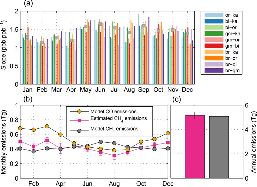
D. Wunch et al.: TCCON-derived European methane                                                                             3971

   The differences between the EDGAR and TNO-                      https://doi.org/10.14291/tccon.ggg2014.karlsruhe01.R1/1182416
MACC_III inventories suggest that the spatial distribution of      (Hase et al., 2014). Bremen data were obtained from
emissions is less certain than the larger-scale emissions, since   https://doi.org/10.14291/tccon.ggg2014.bremen01.R0/1149275
the total carbon monoxide and methane emissions between            (Notholt et al., 2014). Garmisch data were obtained from
the inventories agree to within 15 % and 2 %, respectively, in     https://doi.org/10.14291/tccon.ggg2014.garmisch01.R0/1149299
                                                                   (Sussmann and Rettinger, 2014). Orléans data were obtained from
the study area, but these estimates can disagree by a factor of
                                                                   https://doi.org/10.14291/tccon.ggg2014.orleans01.R0/1149276
2 on city-level scales.                                            (Warneke et al., 2014). Bialystok data were obtained from
   If we assume that the national-scale methane emissions are      https://doi.org/10.14291/tccon.ggg2014.bialystok01.R1/1183984
correctly reported in EDGAR and TNO-MACC_III, our re-              (Deutscher et al., 2017). The Emissions Database for
sults indicate that the methane emissions in the region are        Global Atmospheric Research (EDGAR) inventory is avail-
incorrectly spatially distributed in the inventories. It could     able from the European Commission Joint Research Cen-
be that point or urban sources outside the study area but          tre (JRC) and the Netherlands Environmental Assessment
within the countries intersected by the study area emit a          Agency (PBL), http://edgar.jrc.ec.europa.eu (last access:
larger proportion of the country-level emissions than previ-       7 April 2017). The GEOS-Chem v12.1.0 model is available
ously thought.                                                     from https://doi.org/10.5281/zenodo.1553349 (The International
                                                                   GEOS-Chem User Community, 2018).

4   Conclusions

Using co-located measurements of methane and carbon
monoxide from five long-running ground-based atmospheric
observing stations, we have shown that in the area of Eu-
rope between Orléans, Bremen, Białystok, and Garmisch-
Partenkirchen, the inventories likely overestimate methane
emissions and point to a large uncertainty in the spatial dis-
tribution (i.e., the spatial disaggregation) of country-level
emissions. However, the magnitude of our inferred methane
emissions relies heavily on the EDGAR v4.3.1 and TNO-
MACC_III carbon monoxide inventories, and thus there is a
need for rigorous validation of the carbon monoxide inven-
tories.
   This study demonstrates the potential of clusters of long-
term ground-based stations monitoring total columns of at-
mospheric greenhouse and tracer gases. It also shows the po-
tential of having co-located measurements of multiple pol-
lutants to derive better estimates of emissions. These types
of observing systems can help policy makers verify that
greenhouse gas emissions are reducing at a rate necessary
to meet regulatory obligations. The atmospheric measure-
ments are agnostic to the source (and country of origin) of
the methane, measuring only what is emitted into the atmo-
sphere in a given area. Thus, they can help validate and re-
veal inadequacies in the current inventories, and, in partic-
ular, how country-wide emission reports are disaggregated
on a grid. To enhance these results, simultaneous measure-
ments of complementary atmospheric trace gases, such as
ethane, acetylene, nitrous oxide, nitrogen dioxide, ammo-
nia, and isotopes, would help distinguish between sources of
methane. This would provide additional valuable information
that would likely improve inventory disaggregation.

Data availability. TCCON data are available from the TC-
CON archive, hosted by the California Institute of Technology
at https://tccondata.org. Karlsruhe data were obtained from

www.atmos-chem-phys.net/19/3963/2019/                                               Atmos. Chem. Phys., 19, 3963–3980, 2019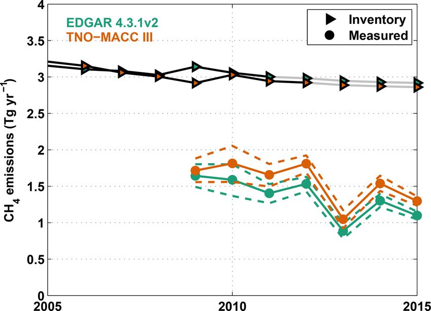
3972                                                                        D. Wunch et al.: TCCON-derived European methane

Appendix A: Filtering

The filtering method was designed to remove days of data
for which the atmospheric air mass was inconsistent between
sites (e.g., a front was passing through or there were signif-
icant stratospheric incursions into the troposphere) and for
years in which there were too few simultaneous measure-
ments at a pair of TCCON stations to compute robust an-
nually representative anomalies.
   To address the consistency of the air mass between sites,
we retained days on which the retrievals of hydrogen fluo-
ride (XHF ) were between 50 ppt and 100 ppt, and deviated by
less than 10 ppt of the median XHF value for all sites on that
day. HF is a trace gas that exists only in the stratosphere, and
thus it serves as a tracer of tropopause height (Washenfelder
et al., 2003; Saad et al., 2014). Since the concentration of
CH4 decreases significantly above the tropopause in the mid-
latitudes, its total column dry-air mole fraction (XCH4 ) is sen-       Figure A2. These are the anomaly slopes (1CH4 /1CO) in
sitive to the tropopause height. Filtering out days on which            ppb ppb−1 for each station pair, for the entire time series. The
XHF varies significantly between sites also ensures that the            anomalies are computed by subtracting data within the same so-
anomalies (and thus the slopes) are minimally impacted by               lar zenith angle bin between two TCCON stations. For more detail,
stratospheric variability. This filter removed less than 5 % of         see Sect. 2 of the main text. The x axis indicates the number of days
                                                                        separating the measurements. The legend identifiers are as follows:
the data.
                                                                        br – Bremen, gm – Garmisch-Partenkirchen, bi – Białystok, or –
   To ensure that the anomalies are representative of the full          Orléans, ka – Karlsruhe.
year, we require that each year has 400 coincident measure-
ments across at least three seasons.

Figure A1. These box plots show the NCEP/NCAR reanalysis long-
term climatological monthly mean wind speeds at the surface (filled
black boxes) and at 850 hPa (open red boxes) in the study area (see
Figs. 1, 7, or 8 for study area maps). The solid black and dashed red
horizontal lines indicate the annual mean wind speed at the surface
and 850 hPa (∼ 1.5 km), respectively. Wind speeds that are aloft (on
average 17 km h−1 ) are significantly swifter than those at the sur-
face (on average 7.5 km h−1 ).

Atmos. Chem. Phys., 19, 3963–3980, 2019                                                    www.atmos-chem-phys.net/19/3963/2019/
D. Wunch et al.: TCCON-derived European methane 3973 Figure A3. These maps show the inventory emissions for the year 2010 in the study area (delineated by the solid straight lines) and the surrounding region. The TCCON stations are marked with black “x” symbols and labeled in black bold font. The countries intersected by, or contained within, the study area are labeled in grey. The map in (a) shows the EDGAR v4.3.1 emissions inventory for carbon monoxide. The map in (b) shows the EDGAR FT2010 emissions inventory for methane. The map in (c) shows the TNO-MACC_III emissions inventory for carbon monoxide. The map in (d) shows the TNO-MACC_III emissions inventory for methane. www.atmos-chem-phys.net/19/3963/2019/ Atmos. Chem. Phys., 19, 3963–3980, 2019
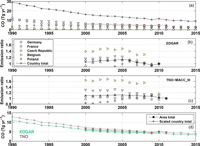
3974                                                                           D. Wunch et al.: TCCON-derived European methane

Figure A4. This four-panel plot shows the methodology for scaling the country-level reported emissions of CO to extrapolate the gridded
inventory emissions to 2015. Panel (a) shows the CO emissions reported by the European Environment Agency (EEA) for the countries
contained within the study area (Germany, France, Czech Republic, Belgium, Luxembourg, and Poland). The black stars with a joining line
represent the summed total from the five countries. The EDGAR (green) and TNO-MACC_III (orange) inventories summed within the study
area are plotted with squares joined by solid lines. Panel (b) shows the ratio between the individual country totals and the EDGAR area
total, normalized to produce an emission ratio of 1 in 2010. The quantity with the least interannual variability in the ratio is from the country
total (black stars with line). Panel (c) shows the ratio between the individual country totals and the TNO-MACC_III area total, normalized
to produce an emission ratio of 1 in 2011. The quantity with the least interannual variability in the ratio is, again, from the country total.
Panel (d) shows the scaled country total, normalized to produce the EDGAR CO emissions for 2010 and the TNO-MACC_III CO emissions
for 2011. This permits us to compute a sensible emission for the study area through to 2015.

Atmos. Chem. Phys., 19, 3963–3980, 2019                                                       www.atmos-chem-phys.net/19/3963/2019/
D. Wunch et al.: TCCON-derived European methane                                                                                 3975

Figure A5. This four-panel plot shows the methodology for scaling the country-level emissions of CH4 reported to the UNFCCC to extrap-
olate the gridded inventory emissions to 2015. The panels and symbols follow the same description as in Fig. A4.

www.atmos-chem-phys.net/19/3963/2019/                                                  Atmos. Chem. Phys., 19, 3963–3980, 2019
3976                                                                D. Wunch et al.: TCCON-derived European methane

Appendix B: Transport time between stations                      the inventory emissions for the years available (2000–2010
                                                                 for EDGAR; 2000–2011 for TNO-MACC_III) in squares.
Figure A1 shows the annual change in monthly mean cli-           Figure A4b–c show the ratio of the country-level emissions
matological wind speeds from the NCEP/NCAR reanalysis            to the area emissions, normalized to 1 for the last year avail-
(Kalnay et al., 1996). These are interpolated to surface pres-   able in the inventory. These panels show that the ratio of
sure and 850 hPa pressures (∼ 1500 m geopotential height)        the summed country total emissions to the emissions from
from model (sigma) surfaces and cover from January 1948          the area of interest is less variable from year to year than
through March 2017. Vertical mixing into the boundary layer      the emissions reported for individual countries. Thus, we
occurs on the timescale of a day or two (Jacob, 1999), and       choose to extrapolate the area emissions using the country
thus the relevant wind speed is between the surface and          total emissions, scaled to the last year of the inventory for
850 hPa. The annual mean surface wind speed is 6 km h−1 ,        the study area.
which gives a mean transit time between Orléans and Bi-             Figure A4d shows the results of using a single scaling fac-
ałystok of 11 days. The annual mean 850 hPa winds are            tor to estimate the study area emissions from the country-
17 km h−1 , which give a shorter mean transit time between       level emissions for each year. We use the summed study area
Orléans and Białystok of 4 days.                                 emissions for the years available, and the extrapolated emis-
   To test whether the transport time impacts the anomalies,     sions through 2015 for subsequent analysis (e.g., Figs. 3 and
we computed the slopes for time lags between sites of 0–         6).
14 days. Figure A2 shows a small change in anomaly slope
as a function of the lag used to calculate the anomalies. This
figure shows that the transport time between TCCON stations
is of negligible importance to the slopes and lends weight to
the decision to compute anomalies from data recorded at two
TCCON stations on the same day.

Appendix C: Computing study area emissions from the
inventories

The study area emissions for 2010 are shown in Fig. A3.
We define the study area as the area bounded by the TC-
CON stations at (clockwise from the west) Orléans, Bremen,
Białystok, and Garmisch-Partenkirchen, which is marked by
the black lines in the figure. To compute the emissions from
the study area, the grid points intersected by and contained
within the solid black lines are summed for each year. The
EDGAR v4.3.1_v2 emissions inventory for CO and FT2010
inventory for CH4 provide estimates for years 2000–2010.
The TNO-MACC_III inventory provides emissions estimates
for both CO and CH4 for the years 2000–2011.

Appendix D: Projecting inventory emissions beyond
2010

Using data from the European Environment Agency National
Database (European Environment Agency, 2016), we extrap-
olate the inventory CO and CH4 emissions for the study area
through 2015. This is done by summing the total emissions
for the five countries that are intersected by the study area
(France, Belgium, Germany, Poland, Luxembourg, Czech
Republic), and normalizing the emissions to the last year of
the inventory (2010 for EDGAR, 2011 for TNO-MACC_III).
Figures A4 and A5 show the process for the EDGAR and
TNO-MACC_III CO and CH4 emissions, respectively.
   Figure A4a shows the reported country-level emissions for
the years 1990–2015, their sum (black stars), and the sum of

Atmos. Chem. Phys., 19, 3963–3980, 2019                                           www.atmos-chem-phys.net/19/3963/2019/
D. Wunch et al.: TCCON-derived European methane 3977
Author contributions. DW designed the study, performed the anal- Chen, J., Viatte, C., Hedelius, J. K., Jones, T., Franklin, J. E., Parker,
ysis, and wrote the paper. DBAJ ran the GEOS-Chem model, sup- H., Gottlieb, E. W., Wennberg, P. O., Dubey, M. K., and Wofsy,
ported by the CO and CH4 work of JAF and JDM. JK and HD- S. C.: Differential column measurements using compact solar-
vdG provided the TNO-MACC_III inventory. GCT helped refine tracking spectrometers, Atmos. Chem. Phys., 16, 8479–8498,
the data analysis methodology. NMD, FH, JN, RS, and TW pro- https://doi.org/10.5194/acp-16-8479-2016, 2016.
vided TCCON data. All coauthors read and provided feedback on Clerbaux, C., Boynard, A., Clarisse, L., George, M., Hadji-Lazaro,
the contents of the paper and helped interpret the results. J., Herbin, H., Hurtmans, D., Pommier, M., Razavi, A., Turquety,
S., Wespes, C., and Coheur, P.-F.: Monitoring of atmospheric
composition using the thermal infrared IASI/MetOp sounder, At-
Competing interests. The authors declare no competing interests. mos. Chem. Phys., 9, 6041–6054, https://doi.org/10.5194/acp-9-
6041-2009, 2009.
Darmenov, A. S. and Silva, A.: The Quick Fire Emissions Dataset
Acknowledgements. The NASA Earth Observatory images were (QFED): Documentation of versions 2.1, 2.2 and 2.4, NASA
prepared by Joshua Stevens, using Suomi National Polar-orbiting Technical Report Series on Global Modeling and Data Assimi-
Partnership (NPP) Visible Infrared Imaging Radiometer (VIIRS) lation, NASA/TM-2015-104606, Tech. Rep. September, NASA,
data from Miguel Román, at NASA’s Goddard Space Flight Cen- Goddard Space Flight Center, Greenbelt, Maryland, 2015.
ter. The authors would like to thank two anonymous reviewers for Deutscher, N. M., Notholt, J., Messerschmidt, J., Weinzierl,
thoughtful comments and suggestions that significantly strength- C., Warneke, T., Petri, C., and Grupe, P.: TCCON data
ened the paper. from Bialystok (PL), Release GGG2014.R1, CaltechDATA,
https://doi.org/10.14291/tccon.ggg2014.bialystok01.r1/1183984,
2017.
Dlugokencky, E. J., Nisbet, E. G., Fisher, R., and Lowry, D.: Global
Review statement. This paper was edited by William Lahoz and re-
atmospheric methane: budget, changes and dangers, Philos. T. R.
viewed by two anonymous referees.
Soc. A., 369, 2058–72, https://doi.org/10.1098/rsta.2010.0341,
2011.
EC-JRC and PBL: Emission Database for Global Atmospheric
Research (EDGAR), release EDGAR v4.3.1_v2 (1970–2010),
References available at: http://edgar.jrc.ec.europa.eu (last access: 16 Octo-
ber 2017), 2016.
Alexe, M., Bergamaschi, P., Segers, A., Detmers, R., Butz, A., EEA: National emissions reported to the Convention on Long-range
Hasekamp, O., Guerlet, S., Parker, R., Boesch, H., Frankenberg, Transboundary Air Pollution (LRTAP Convention) (database),
C., Scheepmaker, R. A., Dlugokencky, E., Sweeney, C., Wofsy, Tech. rep., available at: http://www.eea.europa.eu/data-and-
S. C., and Kort, E. A.: Inverse modelling of CH4 emissions maps/data/national-emissions- reported-to-the-convention-on-
for 2010–2011 using different satellite retrieval products from long-range-transboundary-air-pollution-lrtap-convention-9 (last
GOSAT and SCIAMACHY, Atmos. Chem. Phys., 15, 113–133, access: 15 November 2017), 2015.
https://doi.org/10.5194/acp-15-113-2015, 2015. Emmons, L. K., Deeter, M. N., Gille, J. C., Edwards, D. P., Attié,
Aydin, M., Verhulst, K. R., Saltzman, E. S., Battle, M. O., Montzka, J.-L., Warner, J., Ziskin, D., Francis, G., Khattatov, B., Yudin,
S. A., Blake, D. R., Tang, Q., and Prather, M. J.: Recent decreases V., Lamarque, J.-F., Ho, S.-P., Mao, D., Chen, J. S., Drummond,
in fossil-fuel emissions of ethane and methane derived from firn J., Novelli, P., Sachse, G., Coffey, M. T., Hannigan, J. W., Ger-
air, Nature, 476, 198–201, https://doi.org/10.1038/nature10352, big, C., Kawakami, S., Kondo, Y., Takegawa, N., Schlager, H.,
2011. Baehr, J., and Ziereis, H.: Validation of Measurements of Pol-
Baker, A. K., Schuck, T. J., Brenninkmeijer, C. A. M., Rauthe- lution in the Troposphere (MOPITT) CO retrievals with air-
Schöch, A., Slemr, F., van Velthoven, P. F. J., and Lelieveld, craft in situ profiles, J. Geophys. Res.-Atmos., 109, D03309,
J.: Estimating the contribution of monsoon-related biogenic https://doi.org/10.1029/2003JD004101, 2004.
production to methane emissions from South Asia using Kona, A., Melica, G., Koffi, B., Iancu, A., Zancanella, P., Ri-
CARIBIC observations, Geophys. Res. Lett., 39, L10813, vas Calvete, S., Bertoldi, P., Janssens-Maenhout, G., and
https://doi.org/10.1029/2012GL051756, 2012. Monforti-Ferrario, F.: Covenant of Mayors: Greenhouse Gas
Bloom, A. A., Bowman, K. W., Lee, M., Turner, A. J., Schroeder, Emissions Achievement and Projections, EUR 28155 EN,
R., Worden, J. R., Weidner, R., McDonald, K. C., and Ja- Publications Office of the European Union, Luxembourg,
cob, D. J.: A global wetland methane emissions and un- https://doi.org/10.2790/11008, 2016.
certainty dataset for atmospheric chemical transport models European Environment Agency: Annual European Union green-
(WetCHARTs version 1.0), Geosci. Model Dev., 10, 2141–2156, house gas inventory 1990–2014 and inventory report 2016,
https://doi.org/10.5194/gmd-10-2141-2017, 2017. Tech. rep., available at: http://www.eea.europa.eu/publications/
Buchwitz, M., Schneising, O., Reuter, M., Heymann, J., european-union-greenhouse-gas-inventory-2013 (last access:
Krautwurst, S., Bovensmann, H., Burrows, J. P., Boesch, H., 26 July 2018), 2016.
Parker, R. J., Somkuti, P., Detmers, R. G., Hasekamp, O. Fisher, J. A., Murray, L. T., Jones, D. B. A., and Deutscher, N.
P., Aben, I., Butz, A., Frankenberg, C., and Turner, A. J.: M.: Improved method for linear carbon monoxide simulation
Satellite-derived methane hotspot emission estimates using a and source attribution in atmospheric chemistry models illus-
fast data-driven method, Atmos. Chem. Phys., 17, 5751–5774,
https://doi.org/10.5194/acp-17-5751-2017, 2017.
www.atmos-chem-phys.net/19/3963/2019/ Atmos. Chem. Phys., 19, 3963–3980, 20193978 D. Wunch et al.: TCCON-derived European methane trated using GEOS-Chem v9, Geosci. Model Dev., 10, 4129– Michelsen, H. A., Clements, C. B., Glaize, P., and Fischer, M. L.: 4144, https://doi.org/10.5194/gmd-10-4129-2017, 2017. Estimating methane emissions from biological and fossil-fuel Fortems-Cheiney, A., Chevallier, F., Pison, I., Bousquet, P., sources in the San Francisco Bay Area, Geophys. Res. Lett., 44, Carouge, C., Clerbaux, C., Coheur, P.-F., George, M., Hurtmans, 1, 486–495, https://doi.org/10.1002/2016GL071794, 2017. D., and Szopa, S.: On the capability of IASI measurements to in- Kalnay, E., Kanamitsu, M., Kistler, R., Collins, W., Deaven, form about CO surface emissions, Atmos. Chem. Phys., 9, 8735– D., Gandin, L., Iredell, M., Saha, S., White, G., Woollen, 8743, https://doi.org/10.5194/acp-9-8735-2009, 2009. J., Zhu, Y., Leetmaa, A., Reynolds, R., Chelliah, M., Frankenberg, C., Thorpe, A. K., Thompson, D. R., Hulley, G., Ebisuzaki, W., Higgins, W., Janowiak, J., Mo, K. C., Kort, E. A., Vance, N., Borchardt, J., Krings, T., Gerilowski, Ropelewski, C., Wang, J., Jenne, R., and Joseph, D.: K., Sweeney, C., Conley, S., Bue, B. D., Aubrey, A. D., The NCEP/NCAR 40-Year Reanalysis Project, B. Am. Hook, S., and Green, R. O.: Airborne methane remote mea- Meteorol. Soc., 77, 437–471, https://doi.org/10.1175/1520- surements reveal heavy-tail flux distribution in Four Cor- 0477(1996)0772.0.CO;2, 1996. ners region, P. Natl. Acad. Sci. USA, 113, 35, 9734–9739, Karion, A., Sweeney, C., Miller, J. B., Andrews, A. E., Com- https://doi.org/10.1073/pnas.1605617113, 2016. mane, R., Dinardo, S., Henderson, J. M., Lindaas, J., Lin, J. Geibel, M. C., Messerschmidt, J., Gerbig, C., Blumenstock, T., C., Luus, K. A., Newberger, T., Tans, P., Wofsy, S. C., Wolter, Chen, H., Hase, F., Kolle, O., Lavrič, J. V., Notholt, J., Palm, S., and Miller, C. E.: Investigating Alaskan methane and carbon M., Rettinger, M., Schmidt, M., Sussmann, R., Warneke, T., and dioxide fluxes using measurements from the CARVE tower, At- Feist, D. G.: Calibration of column-averaged CH4 over Euro- mos. Chem. Phys., 16, 5383–5398, https://doi.org/10.5194/acp- pean TCCON FTS sites with airborne in-situ measurements, At- 16-5383-2016, 2016. mos. Chem. Phys., 12, 8763–8775, https://doi.org/10.5194/acp- Kort, E. A., Eluszkiewicz, J., Stephens, B. B., Miller, J. B., Gerbig, 12-8763-2012, 2012. C., Nehrkorn, T., Daube, B. C., Kaplan, J. O., Houweling, S., and Hase, F., Blumenstock, T., Dohe, S., Gross, J., and Wofsy, S. C.: Emissions of CH4 and N2 O over the United States Kiel, M.: TCCON data from Karlsruhe (DE), Release and Canada based on a receptor-oriented modeling framework GGG2014R1, TCCON data archive, hosted by CaltechDATA, and COBRA-NA atmospheric observations, Geophys. Res. Lett., https://doi.org/10.14291/tccon.ggg2014.karlsruhe01.R1/1182416, 35, 1–5, https://doi.org/10.1029/2008GL034031, 2008. 2014. Kort, E. A., Andrews, A. E., Dlugokencky, E. J., Sweeney, C., Hase, F., Frey, M., Blumenstock, T., Groß, J., Kiel, M., Kohlhepp, Hirsch, A., Eluszkiewicz, J., Nehrkorn, T., Michalak, A. M., R., Mengistu Tsidu, G., Schäfer, K., Sha, M. K., and Orphal, J.: Stephens, B. B., Gerbig, C., Miller, J. B., Kaplan, J., Houwel- Application of portable FTIR spectrometers for detecting green- ing, S., Daube, B. C., Tans, P. P., and Wofsy, S. C.: Atmospheric house gas emissions of the major city Berlin, Atmos. Meas. constraints on 2004 emissions of methane and nitrous oxide in Tech., 8, 3059–3068, https://doi.org/10.5194/amt-8-3059-2015, North America from atmospheric measurements and a receptor- 2015. oriented modeling framework, J. Integr. Environ. Sci., 7, 125– Hausmann, P., Sussmann, R., and Smale, D.: Contribution of 133, https://doi.org/10.1080/19438151003767483, 2010. oil and natural gas production to renewed increase in atmo- Kort, E. A., Frankenberg, C., Miller, C. E., and Oda, T.: Space-based spheric methane (2007–2014): top-down estimate from ethane Observations of Megacity Carbon Dioxide, Geophys. Res. Lett., and methane column observations, Atmos. Chem. Phys., 16, 39, 1–5, https://doi.org/10.1029/2012GL052738, 2012. 3227–3244, https://doi.org/10.5194/acp-16-3227-2016, 2016. Kort, E. A., Frankenberg, C., Costigan, K. R., Lindenmaier, R., Hopkins, F. M., Kort, E. A., Bush, S. E., Ehleringer, J. R., Dubey, M. K., and Wunch, D.: Four corners: The largest US Lai, C.-T., Blake, D. R., and Randerson, J. T.: Spatial pat- methane anomaly viewed from space, Geophys. Res. Lett., 41, terns and source attribution of urban methane in the Los 6898–6903, https://doi.org/10.1002/2014GL061503, 2014. Angeles Basin, J. Geophys. Res.-Atmos., 121, 2490–2507, Kuenen, J. J. P., Visschedijk, A. J. H., Jozwicka, M., and De- https://doi.org/10.1002/2015JD024429, 2016. nier van der Gon, H. A. C.: TNO-MACC_II emission inven- Houweling, S., Krol, M., Bergamaschi, P., Frankenberg, C., Dlu- tory; a multi-year (2003–2009) consistent high-resolution Euro- gokencky, E. J., Morino, I., Notholt, J., Sherlock, V., Wunch, pean emission inventory for air quality modelling, Atmos. Chem. D., Beck, V., Gerbig, C., Chen, H., Kort, E. A., Röck- Phys., 14, 10963–10976, https://doi.org/10.5194/acp-14-10963- mann, T., and Aben, I.: A multi-year methane inversion us- 2014, 2014. ing SCIAMACHY, accounting for systematic errors using TC- Maasakkers, J. D., Jacob, D. J., Sulprizio, M. P., Turner, A. J., CON measurements, Atmos. Chem. Phys., 14, 3991–4012, Weitz, M., Wirth, T., Hight, C., DeFigueiredo, M., Desai, M., https://doi.org/10.5194/acp-14-3991-2014, 2014. Schmeltz, R., Hockstad, L., Bloom, A. A., Bowman, K. W., Jacob, D. J.: Introduction to Atmospheric Chemistry, Princeton Uni- Jeong, S., and Fischer, M. L.: Gridded National Inventory of U.S. versity Press, Princeton, New Jersey, 1999. Methane Emissions, Environ. Sci. Technol., 50, 13123–13133, Jacob, D. J., Crawford, J. H., Kleb, M. M., Connors, V. S., Ben- https://doi.org/10.1021/acs.est.6b02878, 2016. dura, R. J., Raper, J. L., Sachse, G. W., Gille, J. C., Em- Maasakkers, J. D., Jacob, D. J., Sulprizio, M. P., Scarpelli, T. R., mons, L., and Heald, C. L.: Transport and Chemical Evo- Nesser, H., Sheng, J.-X., Zhang, Y., Hersher, M., Bloom, A. lution over the Pacific (TRACE-P) aircraft mission: Design, A., Bowman, K. W., Worden, J. R., Janssens-Maenhout, G., and execution, and first results, J. Geophys. Res., 108, 9000, Parker, R. J.: Global distribution of methane emissions, emis- https://doi.org/10.1029/2002JD003276, 2003. sion trends, and OH concentrations and trends inferred from Jeong, S., Cui, X., Blake, D. R., Miller, B., Montzka, S. A., An- an inversion of GOSAT satellite data for 2010–2015, Atmos. drews, A., Guha, A., Martien, P., Bambha, R. P., LaFranchi, B., Atmos. Chem. Phys., 19, 3963–3980, 2019 www.atmos-chem-phys.net/19/3963/2019/
You can also read