Net CO2 fossil fuel emissions of Tokyo estimated directly from measurements of the Tsukuba TCCON site and radiosondes - Atmos. Meas. Tech
←
→
Page content transcription
If your browser does not render page correctly, please read the page content below
Atmos. Meas. Tech., 13, 2697–2710, 2020
https://doi.org/10.5194/amt-13-2697-2020
© Author(s) 2020. This work is distributed under
the Creative Commons Attribution 4.0 License.

Net CO2 fossil fuel emissions of Tokyo estimated directly from
measurements of the Tsukuba TCCON site and radiosondes
Arne Babenhauserheide1,a , Frank Hase1 , and Isamu Morino2
1 IMK-ASF,   Karlsruhe Institute of Technology (KIT), Karlsruhe, Germany
2 National Institute for Environmental Studies (NIES), Tsukuba, Japan
a now at: Disy Informationssysteme GmbH, Karlsruhe, Germany

Correspondence: Arne Babenhauserheide (arne_bab@web.de)

Received: 6 July 2018 – Discussion started: 5 October 2018
Revised: 17 February 2020 – Accepted: 1 April 2020 – Published: 27 May 2020

Abstract. We present a simple statistical approach for es-          The goal of this study is not to calculate the best possible
timating the greenhouse gas emissions of large cities using      estimate of CO2 emissions but to describe a simple method
accurate long-term data of column-averaged greenhouse gas        which can be replicated easily and uses only observation
abundances collected by a nearby FTIR (Fourier transform         data.
infrared) spectrometer. This approach is then used to esti-
mate carbon dioxide emissions from Tokyo.
   FTIR measurements by the Total Carbon Column Observ-
ing Network (TCCON) derive gas abundances by quantita-           1   Introduction
tive spectral analysis of molecular absorption bands observed
in near-infrared solar absorption spectra. Consequently these    Anthropogenic emissions of carbon dioxide are the strongest
measurements only include daytime data.                          long-term control on global climate (Collins et al., 2013,
   The emissions of Tokyo are derived by binning measure-        Fig. 12.3, p. 1046), and the Paris agreement “recognizes the
ments according to wind direction and subtracting measure-       important role of providing incentives for emission reduc-
ments of wind fields from outside the Tokyo area from mea-       tion activities, including tools such as domestic policies and
surements of wind fields from inside the Tokyo area.             carbon pricing“ (UNFCCC secretariat, 2015). Implementing
   We estimate the average yearly carbon dioxide emissions       carbon pricing policies is widely regarded as an effective tool
from the area of Tokyo to be 70 ± 21 ± 6 MtC yr−1 between        for reducing emissions. Such measures also motivate the de-
2011 and 2016, calculated using only measurements from           velopment of new approaches for accurate measurements of
the TCCON site in Tsukuba (north-east of Tokyo) and wind-        carbon emissions (Kunreuther et al., 2014, chapters 2.6.4 and
speed data from nearby radiosondes at Tateno. The uncer-         2.6.5, pp. 181ff).
tainties are estimated from the distribution of values and un-      The carbon dioxide footprint of large-scale fossil-fuel-
certainties of parameters (±21) and from the differences be-     burning emitters like power plants or heating and personal
tween fitting residuals with polynomials or with sines and       transport in megacities has been retrieved from satellite
cosines (±6).                                                    (Hakkarainen et al., 2016; Hammerling et al., 2012; Ichii
   Our estimates are a factor of 1.7 higher than estimates       et al., 2017; Deng et al., 2014; Nassar et al., 2017; Hedelius
using the Open-Data Inventory for Anthropogenic Carbon           et al., 2018) and from ground-based differential measure-
dioxide emission inventory (ODIAC), but when results are         ments using multiple mobile total column instruments (Hase
scaled by the expected daily cycle of emissions, measure-        et al., 2015; Chen et al., 2016; Butz et al., 2017; Viatte
ments simulated from ODIAC data are within the uncertainty       et al., 2017; Vogel et al., 2019; Luther et al., 2019). In-
of our results.                                                  verse modelling allows the coupling of in situ measurements
                                                                 (which only capture enhancements in mixing ratio close to
                                                                 the ground) with atmospheric transport for similar investiga-

Published by Copernicus Publications on behalf of the European Geosciences Union.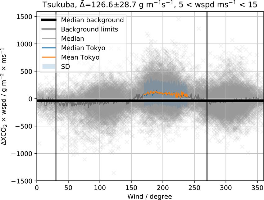
2698                                                              A. Babenhauserheide et al.: Tokyo emissions from TCCON

tions (e.g. Basu et al., 2011; Meesters et al., 2012; van der
Velde et al., 2014; Babenhauserheide et al., 2015; van der
Laan-Luijkx et al., 2017), but due to short mission times of
satellites and differential measurement campaigns and high
uncertainties when using in situ data, long-term changes in
emissions are typically derived from economic fossil fuel and
energy consumption data (e.g. Bureau of the Environment
Tokyo, 2010; Andres et al., 2011; van der Velde et al., 2014;
Le Quéré et al., 2015, 2016).
   The Total Carbon Column Observing Network (TCCON;
Toon et al., 2009; Wunch et al., 2011), described in Sect. 2,
provides highly accurate and precise total column mea-
surements of carbon dioxide mixing ratios with multi-year
records of consistently derived data.
   The aim of our study is to provide an estimate of the CO2
emissions of Tokyo, Japan, by correlating measured XCO2
with wind speed and direction, resulting in a measurement-         Figure 1. Detrending and deseasonalization of the XCO2 total col-
driven approach to derive the annual carbon dioxide emis-          umn measurements in Tsukuba, Japan. The data shown are indi-
sions of Tokyo city (Japan). The main emission sources of          vidual measurements. The trend (shown as a red “trend” line) is
Tokyo are transport, residential, and industry, with about         removed with a linear least-squares fit to the data from background
half the emissions coming from the large coal- and gas-fired       directions between 1 January 2012 and 1 January 2016 (denoted
power plants on the east side of Tokyo Bay, south-east of          by the yellow and magenta vertical lines), the seasonal cycle from
Tokyo city (Bureau of the Environment Tokyo, 2010). The            the signal due to photosynthesis, respiration, and decay (shown as
quality of the data and long time series of available data en-     “yearly cycle fit, degree 6”) is removed by fitting a polynomial of
able us to infer fluxes from the measurements by statistical       degree 6 to the combined yearly cycles of the detrended data. De-
                                                                   gree 6 was chosen empirically to minimize structure in the residuum
matching of measurements to wind directions without being
                                                                   over all TCCON sites.
dominated by measurement noise. We use 4 years of mea-
surements at the TCCON site at Tsukuba, Japan, along with
radiosonde measurements of daily local wind profiles.              of these measurements is better than 0.1 %, as shown by
   This method provides an approach to estimate city emis-         Messerschmidt et al. (2011). Since our study restricts itself
sions which is inexpensive when compared to satellite mis-         to a single station and the uncertainty budget is dominated
sions while being easy to reproduce and to establish, and it is    by other factors, we can ignore any potential minor calibra-
suitable for long-term monitoring. Compared to still cheaper       tion bias of the selected station or the whole network.
in situ measurements, the method has the advantage of di-             Our study uses the current dataset of column-averaged
rectly measuring all emissions from a city in the air column,      carbon dioxide abundances generated with GGG2014 from
while ground-based in situ measurements only capture emis-         solar absorption spectra recorded at the Tsukuba TCCON
sions in the lowermost part of the air profile.                    station, Japan (Ohyama et al., 2009; Morino et al., 2016).
   This publication shows that emissions can be estimated          Publicly available data from Tsukuba at the TCCON data
from 4 years of data. Continued measurements will allow            site used in our study (referenced from the “Code and
tracking of the change in emissions.                               data availability” section) extend from 4 August 2011 to
                                                                   30 March 2016. The coordinates of the Tsukuba TCCON
                                                                   site are 36.05◦ N, 140.12◦ E, and the altitude is 31 m. Further
2   Observations                                                   information about the TCCON site in Tsukuba is available
                                                                   from the TCCON wiki.1 In addition to concentration data
The column data from TCCON currently provides the most             of trace gases, the station provides wind direction and speed
precise and accurate remote-sensing measurements of the            measured at the rooftop of the observatory.
column-averaged CO2 abundances. The average station-to-
station bias is less than 0.3 ppm (Messerschmidt et al., 2010).
   The stations of the TCCON network measure the absorp-           3   Removing trend and natural cycles
tion of CO2 and other molecular species using the sun as
the background radiation source (Wunch et al., 2011). Di-          The approach chosen in this paper to estimate the CO2 emis-
viding the retrieved column amount of the target species by        sions of Tokyo is to separate CO2 measurements by the wind
the co-observed column amount of O2 yields a pressure-
independent measure for the concentration of carbon diox-              1 The TCCON wiki for the Tsukuba site can be found at https:
ide in the dry atmospheric column (XCO2 ). The precision           //tccon-wiki.caltech.edu/Sites/Tsukuba (last access: 21 May 2020).

Atmos. Meas. Tech., 13, 2697–2710, 2020                                              https://doi.org/10.5194/amt-13-2697-2020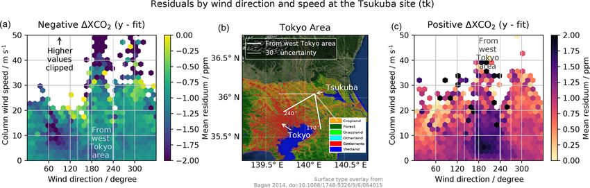
A. Babenhauserheide et al.: Tokyo emissions from TCCON                                                                           2699

                                                                       the data analysis are available in Sect. S1 of the Supple-
                                                                       ment (emissions-tokyo-auxiliary.pdf) of our study. Fitting the
                                                                       yearly cycle only against background directions creates arte-
                                                                       facts; therefore this was avoided. Figures 1 and 2 show the
                                                                       fits and residuals resulting from the process. The calculations
                                                                       only use data provided directly from the TCCON network.
                                                                       The degrees of the fits were chosen empirically (by man-
                                                                       ual adjustment) to minimize the residuals over data from all
                                                                       TCCON sites available in 2016: polynomial fits with degrees
                                                                       between 3 and 9 were tested for the yearly cycle, and the
                                                                       residuals were checked for all TCCON sites. Degrees higher
                                                                       than 6 increased artefacts, and lower degrees increased the
                                                                       overall size of residuals.

                                                                       4   Directional dependence of remaining differences
Figure 2. To remove a potential bias from correlation of wind di-      To calculate the carbon source of Tokyo, the residuals gen-
rection with daytime, which would couple in the signal from photo-     erated by applying the procedures described in Sect. 3 are
synthesis and respiration, the daily cycle is removed by fitting and
                                                                       binned by wind direction and speed, as shown in Fig. 3. A
subtracting a polynomial of degree 3. Degree 3 was chosen empiri-
                                                                       major source of uncertainty in this endeavour is the actual
cally. The fit has low R 2 because the data are dominated by noise.
                                                                       extent of Tokyo in wind directions. This extent was chosen to
                                                                       be 170 to 240◦ as seen from the TCCON site in Tsukuba, fol-
                                                                       lowing the hexbin averages shown in the right panel in Fig. 3.
direction for which they were measured. To make measure-
                                                                       The data in Fig. 3 are separated into positive and negative to
ments from different wind directions comparable, they must
                                                                       ease identification of the limits for emissions from the Tokyo
be made accessible for simple statistical analysis; therefore
                                                                       area. The quantitative evaluation uses both positive and nega-
the first step is to remove trends as well as yearly and daily
                                                                       tive residuals. Within these directional delimiters, all bins in
cycles.
                                                                       the interval with wind speeds between 5 and 15 m s−1 con-
   Column-averaged atmospheric CO2 abundances are dom-
                                                                       tain enhanced concentrations of CO2 . A perfect definition of
inated by seasonal variations and a yearly rise of about
                                                                       these limits is not possible in the scheme presented here be-
2.0 ppm per year (Hartman et al., 2013, p. 167 in
                                                                       cause the area can only be delimited orthogonally to the wind
Sect. 2.2.1.1.1). Additionally there is an average daily cy-
                                                                       direction measured in Tsukuba. In the parallel direction the
cle of about 0.3 ppm in the densely measured daytime be-
                                                                       only limit is changes in wind direction over time: if wind
tween 02:00 UTC and 07:00 UTC (local time between 11:00
                                                                       speed is low enough that on average a direction change oc-
and 16:00 GMT+9). To allow direct comparisons of values
                                                                       curs before the air reaches Tsukuba, then concentration mea-
from different times of year and times of day, these cy-
                                                                       surements from background locations and from Tokyo aver-
cles are removed by fitting and subtracting polynomials from
                                                                       age out. This is indicated by the weaker enhancement seen
the data: linear for the trend, degree 6 for the yearly cycle
                                                                       for wind speeds below 5 m s−1 .
(roughly equivalent to granularity every 2 months), and de-
                                                                          Using 1XCO2 , a measure proportional to the carbon diox-
gree 3 (roughly 3 h granularity) for the daily cycle.
                                                                       ide column enhancement, and the effective wind speed as-
   Polynomials are used in this estimation to make the
                                                                       cribed to these enhancements from the direction of Tokyo al-
method as easy to implement as possible. Section S2 of
                                                                       lows estimation of the emission source of Tokyo (described
the auxiliary material of our study (Babenhauserheide et al.,
                                                                       further in Sect. 5). However, the directly measured wind
2020) provides results from an alternate implementation us-
                                                                       speed which is provided by the TCCON network only pro-
ing harmonics instead, which gives comparable results.
                                                                       vides an approximate indication of the effective wind speed
   The trend is fitted against measurements from background
                                                                       and direction in the altitude range carrying the enhanced car-
directions, but the yearly and daily cycle is fitted against mea-
                                                                       bon dioxide (similar to the effects discussed by Chen et al.,
surements from all directions, so the fitting might remove a
                                                                       2016, for differential measurements of the emissions). For
certain amount of the actual annual and daily cycle of emis-
                                                                       this study, the required effective wind speed is estimated
sions. However, the impact of this fitting in final estimates
                                                                       from radiosonde data.
is limited to wind directions correlated with the cycle, since
uncorrelated differences get reduced in statistical aggrega-
tion. Such a correlation between wind direction and the time
of day exists, but mainly outside the densely measured day-
time; a graph verifying this and the programmes applied for

https://doi.org/10.5194/amt-13-2697-2020                                                 Atmos. Meas. Tech., 13, 2697–2710, 2020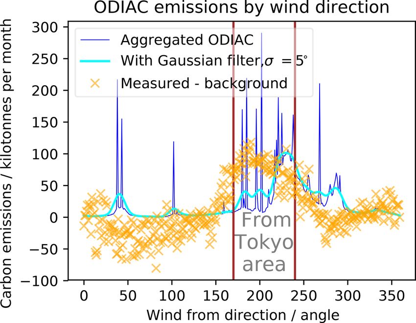
2700                                                                    A. Babenhauserheide et al.: Tokyo emissions from TCCON

Figure 3. Panel (b) shows a map of Tokyo and its surroundings, retrieved from an ArcGIS REST service (retrieved as EPSG:4301
using a ESRI_Imagery_World_2D request to http://server.arcgisonline.com/ArcGIS, last access: 12 February 2020, via the basemap li-
brary in Matplotlib (Hunter, 2007) as described at http://basemaptutorial.readthedocs.io/en/latest/backgrounds.html#arcgisimage, last ac-
cess: 17 May 2020. Used with permission (permission for publication of this graph under Creative Commons attribution license granted by
Esri). © Authors for panels (a) and (c). Panel (b) is used by permission. © Esri, ArcGIS. (b) uses surface type overlays by Bagan 2014
(https://doi.org/10.1088/1748-9326/9/6/064015). All panels distributed under the Creative Commons Attribution 4.0 License.) with an over-
lay indicating the surface type. The colours in the overlay visualize land use and settlement density (taken from Bagan and Yamagata, 2014).
It clearly shows decreasing population density with distance from Tokyo city, along with the long tail of Tokyo settlements towards the
north-west. Close by Tokyo Bay in the lower centre of the map, at the south-east perimeter of Tokyo and on the opposite shore, there are
multiple coal and gas power plants. The Tokyo city centre and the position of the TCCON site in Tsukuba are marked along with white lines
which define an opening angle for incoming wind at Tsukuba which is interpreted as coming from the Tokyo area, along with additional
widening by 30◦ as an estimate of the actual origin of transported CO2 arriving at Tsukuba from the given wind direction. These white lines
denoting the incoming wind angle limits are reproduced in (c) and (a) as delimiting directions in which the wind blows from the west Tokyo
area. Panel (c) shows the positive half of the residuals from Fig. 2, binned by wind direction and strength. The colour represents the mean
value of the positive residuals within the bin. Panel (a) shows the negative half of the residuals from Fig. 2, binned by wind direction and
strength. The colour represents the mean value of the negative residuals within the bin. The black arrow at the upper edge of (a) indicates that
values for wind speeds above 50 m s−1 have been left out to focus on the area between 5 and 15 m s−1 used in the later evaluation. Displaying
residuals which are lower than zero in a different graph than residuals which are higher than zero aids visual detection of emissions, because
it separates the features of CO2 sinks (lower than zero) from CO2 sources (higher than zero). The strongly negative values in (a) at a wind
direction around 60◦ might be due to biospheric drawdown of CO2 by woodland, but since the focus of this publication is the emissions
from Tokyo, those values will not be evaluated further here. The split of the dataset applied here is purely for visualization: in the following
calculations and graphs, negative and positive residuals are used together.

Effective wind speed                                                      service from NOAA2 as described in the auxiliary material
                                                                          (Babenhauserheide et al., 2020). Since the calculations in
                                                                          this publication only use data from measurements with wind
                                                                          speeds of at least 5 m s−1 , 5 h suffices for all trajectories orig-
The wind speed at the station is measured close to the ground.            inating in Tokyo that reach Tsukuba. All the parameters used
The effective speed of the air column however depends on the              are contained in the graphs in Sect. 5 of the Supplement. The
wind speed higher up in the atmosphere. Estimating the wind               HYSPLIT profiles show that most air parcels from Tokyo
speed of air with enhanced carbon dioxide concentrations                  arriving at Tsukuba are contained within the lowest 1000 m
due to emissions from Tokyo therefore requires taking the                 of the atmosphere. Therefore calculating the effective wind
difference in height of the measured concentrations and the               speed of the column with enhanced concentrations only re-
measured wind speed into account. To this end, the ground                 quires wind speed measurements in this part of the atmo-
wind speed v can be replaced by the density-weighted av-                  sphere.
erage wind speed profile within the boundary layer. To cal-                  Direct measurements of the wind speed profile are avail-
culate the required altitude extension of this profile, forward           able from radiosondes. Radiosonde data from Tateno, Japan,
trajectories from Tokyo for 5 to 15 h were calculated with                Ibaraki Prefecture, 36.06◦ N, 140.13◦ E, altitude 27 m, sit-
the HYbrid Single-Particle Lagrangian Integrated Trajectory               uated close to Tsukuba station, provide 7 years of mea-
model (HYSPLIT; Stein et al., 2015) using the Real-time
Environmental Applications and Display sYstem (READY;                         2 The HYSPLIT-WEB online service is available at https://ready.
Rolph et al., 2017), accessed via the HYSPLIT-WEB online                  arl.noaa.gov/HYSPLIT.php (last access: 21 May 2020).

Atmos. Meas. Tech., 13, 2697–2710, 2020                                                      https://doi.org/10.5194/amt-13-2697-2020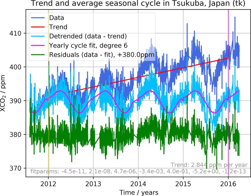
A. Babenhauserheide et al.: Tokyo emissions from TCCON                                                                              2701

surements from 2009 to 2016. The data were retrieved                s⊥ ,
from the Atmospheric Soundings site at the University of
Wyoming (http://weather.uwyo.edu/upperair/sounding.html,            A = v · s⊥ ,                                                     (2)
last access: 21 May 2020). One example of these datasets is
by Ijima (2016). Further details are available in the auxiliary     this source can be derived from the mean total column
material, provided in Babenhauserheide et al. (2020).               enhancement of XCO2 1 = 127 ± 29 gCO2 ms−1 shown in
   Figure 4 visualizes the variability of the wind speed pro-       Fig. 5 via
file weighted by atmospheric pressure from the radiosonde
                                                                    ST = Em A ≈ s⊥ 1.                                                (3)
data measured at the Tateno site. The average wind speed in
the profile with a lower limit of 31 m and an upper limit of        The perpendicular spread s⊥ is calculated by assuming that
1000 m is used to derive daily scaling factors from the ground      total columns of carbon dioxide from the Tokyo area are
wind speed to the average profile wind speed. These scaling         transported to the measurement location without effective di-
factors are applied to the ground wind speed measured at the        vergence perpendicular to the wind direction and assuming
TCCON site in Tsukuba to estimate the effective wind speed          roughly circular city structure. Therefore this spread can be
of the volume of air with enhanced carbon dioxide concen-           approximated from the distance between the Tokyo city cen-
tration in the total column.                                        tre and the TCCON measurement site in Tsukuba:
   These scaling factors are provided in the auxiliary mate-
rial but provide a significant source of uncertainty, since their                                 1α
                                                                    s⊥ ≈ 2π · sTsukuba−Tokyo ·        ,                              (4)
use rests on the assumption of uniform mixing of the carbon                                      360◦
emissions across the boundary layer. The forward trajectory
                                                                    with 1α the opening angle of the limits of wind directions
calculations with HYSPLIT provided in the Supplement sug-
                                                                    associated with Tokyo and sTsukuba−Tokyo ≈ 52km. The city
gest that a 50 km transport distance suffices for particles to
                                                                    centre of Tokyo was chosen to be at the palace (35.6825◦ N,
reach the top of the boundary layer, but they do not prove that
                                                                    139.7521◦ E), between the densely populated area and the
this suffices to generate a uniform CO2 mixing ratio. There-
                                                                    power plants on the other side of Tokyo Bay. Treating 170 to
fore, as also seen by Chen et al. (2016), the unknown actual
                                                                    240◦ as the wind direction coming from Tokyo, this yields a
transport pathway of emitted CO2 to the measurement loca-                                                70◦
                                                                    perpendicular spread of 2π ·52 km· 360  ◦ = 64 km = 64 000 m.
tion is a significant source of uncertainty of the results.
                                                                    The choice of the palace is arbitrary because the actual “cen-
                                                                    tre of mass” of the emissions of Tokyo is unknown. Section 6
                                                                    estimates the uncertainty due to this arbitrary choice.
5   Estimated carbon source of Tokyo
                                                                       For the approximation in Eq. (3), the angle-integrated
                                                                    Em A is collected into contributions from different wind di-
Figure 5 shows the data used to calculate 1, the mean total
                                                                    rections as shown in Eq. (5):
column enhancement of XCO2 . 1 is derived from the XCO2
residuals, the result of subtracting the trend and fits from the             Zα1                         Zα1
yearly and daily cycle as described in Sect. 3: the median to-                                  s⊥
                                                                    Em A =         Em,α Aα dα =    ·           Em,α vα dα = s⊥ 1.    (5)
tal column residual from background wind directions (cho-                                       1α
                                                                             α0                          α0
sen as 270 to 30◦ , using 0◦ from north, clockwise, following
meteorological conventions) is subtracted from the target di-       Therefore the source of Tokyo can be derived from the mean
rection residuals, and then the result is multiplied by the wind    enhancement 1 as
speed during the time of measurement. Finally it is converted
from measured total column concentration CCO2 ,t,col to total       ST = 1 · s⊥ = 127 ± 29 gCO2 ms−1 · 64 000 m
column mass mCO2 ,col using equations from Appendix A at               = 8.1 ± 1.9 tCO2 s−1 .                                        (6)
time t and angle α.
   To calculate the carbon source of Tokyo  ST , the measured     The given uncertainty is taken from the standard deviation as
total column enhancement Em (in gCO2 ) needs to be mul-             shown in Fig. 5.
tiplied with the area affected per second by the emission             For comparison with city emission inventories, the CO2
source from within the Tokyo area, A (m2 s−1 ):                     source is scaled to yearly carbon emissions.

ST = Em · A.                                                 (1)                         MC
                                                                    ST ,C,yearly = 1          s⊥ · s yr−1                            (7)
                                                                                        MCO2
By separating the affected area per second A into the wind                                       12 h       i
speed of the volume of air with enhanced concentrations at                        = 127 ± 29 ·        g ms−1 · 64 000 m
                                                                                                 44
the measurement location v (approximately the average col-
umn wind speed within the boundary layer, 0–1000 m), v and                        · 31 557 600 s yr−1                                (8)
                                                                                                    −1
the spread of the Tokyo area perpendicular to the wind speed                      = 70 ± 16 MtC yr                                   (9)

https://doi.org/10.5194/amt-13-2697-2020                                                Atmos. Meas. Tech., 13, 2697–2710, 2020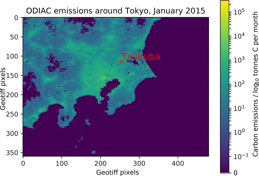
2702                                                                   A. Babenhauserheide et al.: Tokyo emissions from TCCON

Figure 4. Wind speed profile statistics (a) and wind direction statistics (b) up to 1000 m at Tateno, Japan, using data from 2009 to 2016, from
the Ijima (2016) dataset. Values are calculated by dividing the wind speed at a given pressure by the wind speed at the lowest level. The box
plots show the median (red line) and the mean (green triangle). A total of 50 % of values are within the box, the whiskers include 95 % of the
values, and the rest are shown as outliers (black circles). The notch in the box shows the uncertainty of the median calculated via resampling.

                                                                                                                     ktC
                                                                                                     = 82 ± 19                            (12)
                                                                                                                 month · degree

                                                                          6   Estimating uncertainties

                                                                          In addition to the statistical uncertainty and the uncertainty
                                                                          of the wind profile discussed in Sect. 4, the estimated emis-
                                                                          sion depends on the assumed extent of the Tokyo area and
                                                                          is limited by the unknown actual distribution of distances of
                                                                          emission sources from the measurement site at Tsukuba.
                                                                             Choosing different opening angles for air from the
                                                                          Tokyo area yields a yearly emission range from 54.0 ±
                                                                          7.4 MtC year−1 when choosing air from the Tokyo area be-
                                                                          tween 180 and 220◦ up to 93±35 MtC year−1 when choosing
                                                                          air from the Tokyo area between 150 and 260◦ . This uncer-
Figure 5. Residuals multiplied by wind speed plotted against the          tainty also plays a role in comparisons, if the actual wind
wind direction for scaled wind speeds between 5 and 15 m s−1 ,            direction higher up in the atmosphere is not distributed sym-
measured by the TCCON site in Tsukuba, Japan. The mean en-
                                                                          metrically around the wind direction at ground.
hancement 1, the mean Tokyo and median Tokyo values and the
standard deviation are calculated for the directions defined as from
                                                                             The distance of emission sources from the TCCON site
Tokyo in Fig. 3. The median background is calculated from the             in Tsukuba affects the estimated spread of the emission re-
residuals outside the background limits (lower than 30◦ or higher         gion perpendicular to the wind direction. This calculation as-
than 270◦ ; limits drawn as vertical lines). The bin size is 1◦ .         sumes a distribution of emission strengths along the wind di-
                                                                          rection symmetrically around a centre given by the distance.
                                                                          This assumption is plausible since the most densely popu-
For comparison with gridded emission inventories in Sect. 7,              lated region of Tokyo extends to the north-west towards the
the CO2 emissions are scaled to average monthly carbon                    prefecture of Saitama. However Bagan and Yamagata (2014)
emissions per wind direction (in 1◦ steps).                               and Oda and Maksyutov (2011, 2016) show a similar exten-
                                                                          sion towards the south, and the power plants are southward
                                MC                 s
Sτ,CO2 ,average,deg,monthly = 1        s⊥ ·                 (10)          of the palace. Assuming an uncertainty of 10 km for the dis-
                               MCO2         month · degree                tance between the centre of mass and the measurement site
                                        hg     i 12  g
                                           CO2           C                increases the uncertainty.
                          = 127 ± 29            ·
                                          ms      44 gCO2
                                                      s                                                             70◦
                          · 914 m · 2 592 000                             ST = 1 · s⊥ = 1 · 2π · 52 ± 10 km ·           = 1 · 64 ± 12.3 km
                                               month · degree                                                      360◦
                                                            (11)                                                                      (13)

Atmos. Meas. Tech., 13, 2697–2710, 2020                                                      https://doi.org/10.5194/amt-13-2697-2020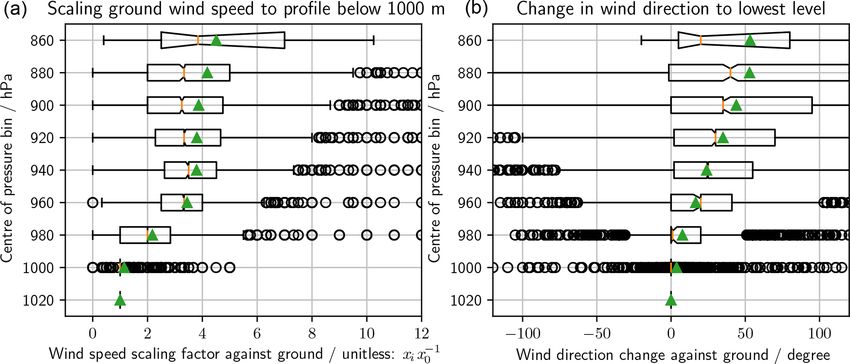
A. Babenhauserheide et al.: Tokyo emissions from TCCON                                                                         2703

   = 127 ± 29 gCO2 ms−1 · 64 000 ± 12 300 m
   = 8.1 ± 2.4 tCO2 s−1                                     (14)
                        −1
   ⇒ 70 ± 21 MtC yr                                         (15)
                 ktC
   ⇒ 82 ± 24              .                                 (16)
             year, degree
This uncertainty needs to be taken into account but can only
be estimated. It gives a contribution of      MtC yr−1 .
   The ground wind speed from TCCON data also varies by
around 30 %, but this is part of the scatter in the data, so it
is already averaged and reported. The scaling factors are cal-
culated daily, so their uncertainty is part of the scatter in the
data, too. Within the relevant pressure region here (860 hPa
and more), the TCCON averaging kernels can vary, but this
is also part of the scatter of the data. Systematic effects could   Figure 6. ODIAC carbon emissions per 1 km × 1 km pixel for Jan-
be a slightly higher sensitivity in the morning and evening,        uary 2015 in log10 scale. This graph is created directly from the
                                                                    1 km × 1 km ODIAC dataset (Oda and Maksyutov, 2011, 2016)
but that is also the time with the least amount of data.
                                                                    to visualize its structure. The model emissions are shown for
   Another source of uncertainty is the accuracy of the back-
                                                                    the area visualized in the middle panel of Fig. 3. The unit is
ground. A bias in the background translates into a bias of the      metric tonnes of carbon per cell and month as described in the
result. For sites with a large forest in one direction but none     README file at http://db.cger.nies.go.jp/dataset/ODIAC/readme/
close to the city, this would have to be taken into account.        readme_2016_20170202.txt (last access: 21 May 2020).
   The fitting procedure can affect the outcome. Repeating
the same calculations with a different fitting procedure based
on sines and cosines (e.g. Thoning et al., 1989), implemented
using the ccgfilt library (referenced in the Code and data
availability section) gives an idea of the impact of the fit-
ting. As shown in Sect. 2 of the auxiliary material (Baben-
hauserheide et al., 2020), this calculation yields 1 = 138 ±
31 gCO2 ms−1 as a source instead of the 127 ± 29 gCO2 ms−1
found with polynomial fits. This corresponds to a relative dif-
ference of 8.3 % which is not captured by the internal vari-
ability of the residuals. For 70 MtC, the absolute difference
is     MtC. The structure of this error is unknown, though;
therefore it is shown separately.
   Consequently the most robust estimate of the emissions of
Tokyo is for yearly carbon emissions of Tokyo

ST,C,yearly = 70 ± 16         MtC yr−1                      (17)

  and for monthly carbon dioxide emissions of Tokyo                 Figure 7. Sum of ODIAC carbon emissions by direction in angular
                                                                    degrees as seen from Tsukuba, Japan. The “aggregated ODIAC”
                                                ktC                 emissions show emissions per direction from the beginning of 2011
Sτ,CO2 ,average,deg,monthly = 82 ± 18                      .
                                            month · degree          to the end of 2016. The Gaussian filter data use a moving average
                                                           (18)     to estimate signals measured at a distance. The measured dataset
                                                                    shows the median residuals from Fig. 5 for comparison.
These values provide an estimate of the source for Tokyo
calculated directly from measurements. The measurements
are only conducted between 00:00 and 08:00 UTC, though,             fluxes which would be derived from measurements through
and the fossil fuel sources of Tokyo might be different during      the day. This would result in a total emission estimate of 60±
nighttime due to reduced human activity. Nassar et al. (2013)       18 MtC yr−1 .
provide hourly scaling factors for fluxes for global models. In        Daily cycle corrected yearly emissions are
the measurement interval these scaling factors are 1.09, 1.11,
1.13, 1.16, 1.16, 1.18, 1.20, 1.21, and 1.188, which gives an       ŜT,C,yearly = 60 ± 18    MtC yr−1 .                        (19)
average factor of 1.16, with the standard deviation given as
0.15. Dividing the fluxes by 1.16 gives an estimate of the

https://doi.org/10.5194/amt-13-2697-2020                                              Atmos. Meas. Tech., 13, 2697–2710, 2020
2704 A. Babenhauserheide et al.: Tokyo emissions from TCCON
7 Comparison with other datasets these fluxes. Pisso et al. (2019) also compare several other
datasets with their source definition.
To compare the results with the high-resolution Open-
Data Inventory for Anthropogenic Carbon dioxide emission
(ODIAC; Oda and Maksyutov, 2011) in version ODIAC2016 8 Conclusions and outlook
(Oda and Maksyutov, 2016), using the regional slice shown
in Fig. 6, measurements are simulated from ODIAC by sum- We find that a single multi-year dataset of precise column
ming emissions by direction as seen from the position of measurements provides valuable insights into the carbon
Tsukuba station. For total emissions, all emissions within emissions of city-scale emitters. The estimated emissions of
the arc spanned by the limits of Tokyo area from 2011 to 70±21±6 MtC yr−1 found for Tokyo have less than 50 % un-
2016 are aggregated; then the sum of the emissions from certainty despite our intentional constraint to use only a ba-
background directions is subtracted. Emissions aggregated sic evaluation scheme which can be repeated on any personal
for each 1◦ angle segment are shown in Fig. 7): computer with publicly available data. While the operation of
! a TCCON station is a major effort, a decade of CO2 column
Tokyo bg
1 2015−12
X X X measurements of comparable quality can be conducted with
EODIAC,t,α − EODIAC,t,β affordable and easier-to-operate mobile spectrometers (see
5 t=2011−01 α β
for example Frey et al., 2019), which opens an avenue for ev-
= 40.4 MtC yr−1 , (20) ery country to measure and evaluate emissions of megacities.
Placing a single total column measurement site in the vicin-
which is around 60 % of the emissions estimated in this pa- ity of major cities can make it possible to estimate their emis-
per from TCCON measurement data and within 2 standard sions purely from these measurements. This can complement
deviations (σ ) of the estimated emissions. With the scaling global source and sink estimates and improve acceptance of
for the time of day of the measurement, ODIAC results lie carbon trading programmes by enabling independent verifi-
within 1 standard deviation of the estimate in this paper. cation of findings.
The peak of the distribution of emissions (from the Tokyo Significant reduction of the uncertainties in these estimates
area) is shifted about 30◦ anticlockwise from the model to without adding more measurement stations would require
measurements. This is within the expected changes due to the taking into account more detailed wind fields from meteoro-
typical shift in wind direction between measurements con- logical models, correcting for the wind direction at different
ducted close to the ground and measurements higher up in the altitudes by using partial columns, more detailed correction
planetary boundary layer (Ekman, 1905). These discrepan- for expected CO2 take-up from the biosphere by wind direc-
cies could be corrected by using more complex atmospheric tion, or correcting for the diurnal cycle of fossil fuel emis-
transport, but that would require every person reproducing sions. These corrections are already taken into account in
the estimates from our study to run such a transport, which source–sink estimates based on inverse modelling of atmo-
would defeat the purpose of our study, namely to provide an spheric transport with biosphere models (e.g. van der Laan-
easily reusable approach for estimating city emissions. Luijkx et al., 2017; Riddick et al., 2017; Massart et al., 2014;
The economic data published by the Bureau of the Envi- Basu et al., 2013); therefore this implementation keeps close
ronment Tokyo (2010) report emissions of 57.7 MtCO2 yr−1 to the simpler evaluation which allows us to use easily acces-
in the fiscal year 2006 for the Tokyo metropolitan area. This sible data, which keeps our findings easy to replicate. A bet-
is equivalent to 15.7 MtC yr−1 and shows a large discrepancy ter classification of uncertainty due to the assumption of uni-
to our results. This discrepancy could stem from different form vertical distribution of the emitted CO2 could be given
definitions for the source area. Part of this discrepancy cannot by measuring highly resolved vertical profiles from aircraft
be reconciled because the method shown in this study cannot downwind of Tokyo.
limit the emission aggregation parallel to the wind direction Further uncertainty reductions can be achieved by estab-
and has around 30◦ uncertainty of the direction, so it also in- lishing several observing sites within and around the source
cludes some emissions from Kanagawa, Saitama, and Chiba, area (e.g. Hase et al., 2015; Turner et al., 2016). This ap-
the prefectures around Tokyo which are part of the greater proach also provides information about the spatial structure
Tokyo area. of emissions and can be used in focused measurement cam-
Pisso et al. (2019) estimate the emissions of Tokyo city as paigns to obtain constraints for evaluation of measurements
22 MtC yr−1 (80 MtCO2 yr−1 ) and of the Tokyo metropoli- with coarser spatial resolution as well as long-term datasets.
tan area as 151 MtC yr−1 (554 MtCO2 yr−1 ). With 70 ± It would eliminate most of the uncertainty in the mean dis-
21 MtC yr−1 (256 ± 77 MtCO2 ) this study lies be- tance between measurement site and emitters.
tween those values, which is to be expected because the Reduction of the bias due to measuring only during day-
definition of the metropolitan area used in Pisso et al. time, while keeping close to direct measurements, could
(2019) includes all the fluxes from the prefectures Kanagawa, be achieved by calculating the diurnal scaling of the emis-
Saitama, and Chiba, while this study only includes part of sion source from CO2 concentration measurements of an
Atmos. Meas. Tech., 13, 2697–2710, 2020 https://doi.org/10.5194/amt-13-2697-2020A. Babenhauserheide et al.: Tokyo emissions from TCCON 2705 in situ instrument or by taking moonlight measurements (Buschmann et al., 2017). To complete this outlook, we would like to suggest that the negative values seen in the left graph of Fig. 3 at a wind direction around 60◦ indicate that it might also be possible to detect biospheric drawdown of CO2 by woodland with just a single total column instrument and that this method can also be used to analyse other greenhouse gases measured by the TCCON network, including methane and carbon monoxide. Residuals for methane are shown in Fig. S6 of the Supple- ment. We conclude that long-term ground-based measurements of column-averaged greenhouse gas abundances with suffi- cient precision for detecting the signals of local emission sources are an effective and cost-efficient approach to im- prove our knowledge about sources and sinks of greenhouse gases. https://doi.org/10.5194/amt-13-2697-2020 Atmos. Meas. Tech., 13, 2697–2710, 2020
2706                                                           A. Babenhauserheide et al.: Tokyo emissions from TCCON

Appendix A: Units and definitions
                                                       p      5
                                                                  −2
 Unit air column mass:         mair,col            =   g × 10     gm
                                                       MCO2 mair,col            −2
 CO2 column mass               mCO2 ,col           =    Mair fcol · CCO2 ,t,col gm
                                                   = mCO2 ,col − mCO2 ,col,seasonal cycle fit − mCO2 ,col,daily cycle fit g m−2 (de-

 Total column residuum:        R
                                                   scribed in Sect. 3)
                                                   = Rfrom Tokyo area − median Rfrom background g m−2

 Enhancement:                  Em
 Molar mass of CO2             MCO2                = 44.0 g mol−1
 Molar mass of dry air         Mair                = 28.9 g mol−1 ,
 Column mass correction        fcol                = 0.9975, following Bannon et al. (1997) to adjust for curved geometry
 Tracer mass                   mgas,col [g],
 Total column dry-air mass     mair,col [g],
 Column concentration          CCO2 ,t,col ppm ,
 Acceleration due to gravity   g [m s−2 ]          (from TCCON a priori),
 Pressure                      p [g m s−2 ].       (with wet-air to dry-air correction)
 Perpendicular spread          s⊥ [m]

Atmos. Meas. Tech., 13, 2697–2710, 2020                                             https://doi.org/10.5194/amt-13-2697-2020
A. Babenhauserheide et al.: Tokyo emissions from TCCON 2707
Code and data availability. All code used and preprocessed data References
in JSON format (as described in https://tools.ietf.org/html/rfc7159,
last access: 21 May 2020) are available in the Supplement (Baben- Andres, R. J., Gregg, J. S., Losey, L., Marland, G., and
hauserheide et al., 2020, https://doi.org/10.5281/zenodo.3845548). Boden, T. A.: Monthly, global emissions of carbon diox-
See the README file in the Supplement for usage information. ide from fossil fuel consumption, Tellus B, 63, 309–327,
All non-included data are publicly available from the TCCON data https://doi.org/10.1111/j.1600-0889.2011.00530.x, 2011.
portal (http://tccondata.org/, last access: 21 May 2020), from the Babenhauserheide, A., Basu, S., Houweling, S., Peters, W., and
ODIAC project odiac.org (http://odiac.org/dataset.html, last access: Butz, A.: Comparing the CarbonTracker and TM5-4DVar data
21 May 2020), and from the Atmospheric Soundings site at the Uni- assimilation systems for CO2 surface flux inversions, Atmos.
versity of Wyoming (http://weather.uwyo.edu/upperair/sounding. Chem. Phys., 15, 9747–9763, https://doi.org/10.5194/acp-15-
html, last access: 21 May 2020). The ccgfilt library is available 9747-2015, 2015.
from NOAA via ftp://ftp.cmdl.noaa.gov/user/thoning/ccgcrv/ (last Babenhauserheide, A., Hase, F., and Morino, I.: Code and Data for
access: 21 May 2020). amt-2018-224, https://doi.org/10.5281/zenodo.3845548, 2020.
Bagan, H. and Yamagata, Y.: Land-cover change analysis in
50 global cities by using a combination of Landsat data
Supplement. The supplement related to this article is available on- and analysis of grid cells, Environ. Res. Lett., 9, 064015,
line at: https://doi.org/10.5194/amt-13-2697-2020-supplement. https://doi.org/10.1088/1748-9326/9/6/064015, 2014.
Bannon, P. R., Bishop, C. H., and Kerr, J. B.: Does
the Surface Pressure Equal the Weight per Unit
Area of a Hydrostatic Atmosphere?, B. Am. Meteo-
Author contributions. IM provided the TCCON data at Tsukuba
rol. Soc., 78, 2637–2642, https://doi.org/10.1175/1520-
station and helped to interpret it; FH helped find working ap-
0477(1997)0782.0.co;2, 1997.
proaches for the evaluation and improving the manuscript; and AB
Basu, S., Houweling, S., Peters, W., Sweeney, C., Machida,
implemented the evaluation, calculated the results, and wrote most
T., Maksyutov, S., Patra, P. K., Saito, R., Chevallier, F.,
of the manuscript.
Niwa, Y., Matsueda, H., and Sawa, Y.: The seasonal cy-
cle amplitude of total column CO2 : Factors behind the
model-observation mismatch, J. Geophys. Res.-Atmos., 116,
Competing interests. The authors have no competing financial in- https://doi.org/10.1029/2011JD016124, 2011.
terests, but Frank Hase and Isamu Morino are working on other Basu, S., Guerlet, S., Butz, A., Houweling, S., Hasekamp, O., Aben,
projects with ground-based total column measurement instruments. I., Krummel, P., Steele, P., Langenfelds, R., Torn, M., Biraud, S.,
Stephens, B., Andrews, A., and Worthy, D.: Global CO2 fluxes
estimated from GOSAT retrievals of total column CO2 , At-
Acknowledgements. Much of the inspiration for this method of mos. Chem. Phys., 13, 8695–8717, https://doi.org/10.5194/acp-
evaluation and the boldness to keep it simple are due to our trea- 13-8695-2013, 2013.
sured colleague Friedrich Klappenbach (especially his evaluation of Bureau of the Environment Tokyo: Tokyo Cap-and-
CO2 in Klappenbach et al., 2015). The simple estimate of effective Trade Program: Japan’s first mandatory emissions
boundary layer wind speed from radiosonde data was suggested by trading scheme, Tech. rep., Tokyo Metropolitan Gov-
Bernhard Vogel. Matthias Frey contributed insights into differential ernment, available at: https://mega.nz/file/pdxXFLxZ#
measurements of the Tokyo source using multiple portable spec- _0vPHK4HFKB8QzDfAtJURL7QMkJt2m1s-1wDr1wUzU4
trometers, as well as fruitful discussions about these evaluations. (last access: 21 May 2020), 2010.
Support for this study was provided by the Bundesministerium Buschmann, M., Deutscher, N. M., Palm, M., Warneke, T.,
für Bildung und Forschung (BMBF) through the ROMIC project, Weinzierl, C., and Notholt, J.: The arctic seasonal cycle of total
with funding for initial work provided by the Emmy Noether Pro- column CO2 and CH4 from ground-based solar and lunar FTIR
gramme of the Deutsche Forschungsgemeinschaft (DFG) through absorption spectrometry, Atmos. Meas. Tech., 10, 2397–2411,
grant BU2599/1-1 (RemoteC). https://doi.org/10.5194/amt-10-2397-2017, 2017.
The article processing charges for this open-access publication Butz, A., Dinger, A. S., Bobrowski, N., Kostinek, J., Fieber, L., Fis-
have been covered by a Research Centre of the Helmholtz Associa- cherkeller, C., Giuffrida, G. B., Hase, F., Klappenbach, F., Kuhn,
tion. J., Lübcke, P., Tirpitz, L., and Tu, Q.: Remote sensing of volcanic
CO2 , HF, HCl, SO2 , and BrO in the downwind plume of Mt.
Etna, Atmos. Meas. Tech., 10, 1–14, https://doi.org/10.5194/amt-
Financial support. The article processing charges for this open- 10-1-2017, 2017.
access publication were covered by a Research Centre of the Chen, J., Viatte, C., Hedelius, J. K., Jones, T., Franklin, J. E., Parker,
Helmholtz Association. H., Gottlieb, E. W., Wennberg, P. O., Dubey, M. K., and Wofsy,
S. C.: Differential column measurements using compact solar-
tracking spectrometers, Atmos. Chem. Phys., 16, 8479–8498,
Review statement. This paper was edited by Helen Worden and re- https://doi.org/10.5194/acp-16-8479-2016, 2016.
viewed by three anonymous referees. Collins, M., Knutti, R., Arblaster, J., Dufresne, J.-L., Fichefet, T.,
Friedlingstein, P., Gao, X., Gutowski, W., Johns, T., Krinner,
G., Shongwe, M., Tebaldi, C., Weaver, A., and Wehner, M.:
Long-term Climate Change: Projections, Commitments and Ir-
https://doi.org/10.5194/amt-13-2697-2020 Atmos. Meas. Tech., 13, 2697–2710, 20202708 A. Babenhauserheide et al.: Tokyo emissions from TCCON reversibility, book section 12, p. 1029–1136, Cambridge Uni- Machimura, T., Matsuura, Y., Mizoguchi, Y., Ohta, T., Mukher- versity Press, Cambridge, United Kingdom and New York, NY, jee, S., Yanagi, Y., Yasuda, Y., Zhang, Y., and Zhao, F.: New USA, https://doi.org/10.1017/CBO9781107415324.024, 2013. data-driven estimation of terrestrial CO2 fluxes in Asia using a Deng, F., Jones, D. B. A., Henze, D. K., Bousserez, N., Bowman, K. standardized database of eddy covariance measurements, remote W., Fisher, J. B., Nassar, R., O’Dell, C., Wunch, D., Wennberg, P. sensing data, and support vector regression, J. Geophys. Res.- O., Kort, E. A., Wofsy, S. C., Blumenstock, T., Deutscher, N. M., Biogeo., 122, 767–795, https://doi.org/10.1002/2016JG003640, Griffith, D. W. T., Hase, F., Heikkinen, P., Sherlock, V., Strong, 2017. K., Sussmann, R., and Warneke, T.: Inferring regional sources Ijima, O.: Radiosonde measurements from station Tateno (2015- and sinks of atmospheric CO2 from GOSAT XCO2 data, At- 12), PANGAEA, https://doi.org/10.1594/PANGAEA.858510, mos. Chem. Phys., 14, 3703–3727, https://doi.org/10.5194/acp- 2016. 14-3703-2014, 2014. Klappenbach, F., Bertleff, M., Kostinek, J., Hase, F., Blumenstock, Ekman, V. W.: On the influence of the earth’s rotation on T., Agusti-Panareda, A., Razinger, M., and Butz, A.: Accurate ocean-currents, available at: https://jscholarship.library.jhu.edu/ mobile remote sensing of XCO2 and XCH4 latitudinal transects bitstream/handle/1774.2/33989/31151027498728.pdf (last ac- from aboard a research vessel, Atmos. Meas. Tech., 8, 5023– cess: 21 May 2020), 1905. 5038, https://doi.org/10.5194/amt-8-5023-2015, 2015. Frey, M., Sha, M. K., Hase, F., Kiel, M., Blumenstock, T., Harig, Kunreuther, H., Gupta, S., Bosetti, V., Cooke, R., Dutt, V., Ha- R., Surawicz, G., Deutscher, N. M., Shiomi, K., Franklin, J. E., Duong, M., Held, H., Llanes-Regueiro, J., Patt, A., Shittu, E., Bösch, H., Chen, J., Grutter, M., Ohyama, H., Sun, Y., Butz, A., and Weber, E.: Integrated Risk and Uncertainty Assessment of Mengistu Tsidu, G., Ene, D., Wunch, D., Cao, Z., Garcia, O., Climate Change Response Policies, chap. 2, pp. 151–206, Work- Ramonet, M., Vogel, F., and Orphal, J.: Building the COllabora- ing Group III to the Fifth Assessment Report of the Intergovern- tive Carbon Column Observing Network (COCCON): long-term mental Panel on Climate Change, 2014. stability and ensemble performance of the EM27/SUN Fourier Le Quéré, C., Moriarty, R., Andrew, R. M., Peters, G. P., Ciais, P., transform spectrometer, Atmos. Meas. Tech., 12, 1513–1530, Friedlingstein, P., Jones, S. D., Sitch, S., Tans, P., Arneth, A., https://doi.org/10.5194/amt-12-1513-2019, 2019. Boden, T. A., Bopp, L., Bozec, Y., Canadell, J. G., Chini, L. P., Hakkarainen, J., Ialongo, I., and Tamminen, J.: Direct space-based Chevallier, F., Cosca, C. E., Harris, I., Hoppema, M., Houghton, observations of anthropogenic CO2 emission areas from OCO- R. A., House, J. I., Jain, A. K., Johannessen, T., Kato, E., Keel- 2, Geophys. Res. Lett., https://doi.org/10.1002/2016GL070885, ing, R. F., Kitidis, V., Klein Goldewijk, K., Koven, C., Landa, 2016. C. S., Landschützer, P., Lenton, A., Lima, I. D., Marland, G., Hammerling, D. M., Michalak, A. M., and Kawa, S. R.: Mapping Mathis, J. T., Metzl, N., Nojiri, Y., Olsen, A., Ono, T., Peng, S., of CO2 at high spatiotemporal resolution using satellite observa- Peters, W., Pfeil, B., Poulter, B., Raupach, M. R., Regnier, P., Rö- tions: Global distributions from OCO-2, J. Geophys. Res., 117, denbeck, C., Saito, S., Salisbury, J. E., Schuster, U., Schwinger, D06306, https://doi.org/10.1029/2011JD017015, 2012. J., Séférian, R., Segschneider, J., Steinhoff, T., Stocker, B. D., Hartmann, D., Klein Tank, A., Rusticucci, M., Alexander, L., Sutton, A. J., Takahashi, T., Tilbrook, B., van der Werf, G. R., Brönnimann, S., Charabi, Y., Dentener, F., Dlugokencky, E., Viovy, N., Wang, Y.-P., Wanninkhof, R., Wiltshire, A., and Zeng, Easterling, D., Kaplan, A., Soden, B., Thorne, P., Wild, N.: Global carbon budget 2014, Earth Syst. Sci. Data, 7, 47–85, M., and Zhai, P.: Observations: Atmosphere and Surface, https://doi.org/10.5194/essd-7-47-2015, 2015. book section 2, p. 159–254, Cambridge University Press, Le Quéré, C., Andrew, R. M., Canadell, J. G., Sitch, S., Kors- Cambridge, United Kingdom and New York, NY, USA, bakken, J. I., Peters, G. P., Manning, A. C., Boden, T. A., Tans, https://doi.org/10.1017/CBO9781107415324.008, 2013. P. P., Houghton, R. A., Keeling, R. F., Alin, S., Andrews, O. D., Hase, F., Frey, M., Blumenstock, T., Groß, J., Kiel, M., Kohlhepp, Anthoni, P., Barbero, L., Bopp, L., Chevallier, F., Chini, L. P., R., Mengistu Tsidu, G., Schäfer, K., Sha, M. K., and Orphal, J.: Ciais, P., Currie, K., Delire, C., Doney, S. C., Friedlingstein, P., Application of portable FTIR spectrometers for detecting green- Gkritzalis, T., Harris, I., Hauck, J., Haverd, V., Hoppema, M., house gas emissions of the major city Berlin, Atmos. Meas. Klein Goldewijk, K., Jain, A. K., Kato, E., Körtzinger, A., Land- Tech., 8, 3059–3068, https://doi.org/10.5194/amt-8-3059-2015, schützer, P., Lefèvre, N., Lenton, A., Lienert, S., Lombardozzi, 2015. D., Melton, J. R., Metzl, N., Millero, F., Monteiro, P. M. S., Hedelius, J. K., Liu, J., Oda, T., Maksyutov, S., Roehl, C. M., Iraci, Munro, D. R., Nabel, J. E. M. S., Nakaoka, S., O’Brien, K., L. T., Podolske, J. R., Hillyard, P. W., Liang, J., Gurney, K. R., Olsen, A., Omar, A. M., Ono, T., Pierrot, D., Poulter, B., Rö- Wunch, D., and Wennberg, P. O.: Southern California megac- denbeck, C., Salisbury, J., Schuster, U., Schwinger, J., Séférian, ity CO2 , CH4 , and CO flux estimates using ground- and space- R., Skjelvan, I., Stocker, B. D., Sutton, A. J., Takahashi, T., Tian, based remote sensing and a Lagrangian model, Atmos. Chem. H., Tilbrook, B., van der Laan-Luijkx, I. T., van der Werf, G. Phys., 18, 16271–16291, https://doi.org/10.5194/acp-18-16271- R., Viovy, N., Walker, A. P., Wiltshire, A. J., and Zaehle, S.: 2018, 2018. Global Carbon Budget 2016, Earth Syst. Sci. Data, 8, 605–649, Hunter, J.: Matplotlib: A 2D Graphics Environment, Comput. Sci. https://doi.org/10.5194/essd-8-605-2016, 2016. Eng., 9, 90–95, https://doi.org/10.1109/MCSE.2007.55, 2007. Luther, A., Kleinschek, R., Scheidweiler, L., Defratyka, S., Ichii, K., Ueyama, M., Kondo, M., Saigusa, N., Kim, J., Alberto, Stanisavljevic, M., Forstmaier, A., Dandocsi, A., Wolff, S., M. C., Ardö, J., Euskirchen, E. S., Kang, M., Hirano, T., Joiner, Dubravica, D., Wildmann, N., Kostinek, J., Jöckel, P., Nickl, A.- J., Kobayashi, H., Belelli Marchesini, L., Merbold, L., Miyata, L., Klausner, T., Hase, F., Frey, M., Chen, J., Dietrich, F., Ne¸cki, A., Saitoh, T. M., Takagi, K., Varlagin, A., Bret-Harte, M. S., J., Swolkień, J., Fix, A., Roiger, A., and Butz, A.: Quantifying Kitamura, K., Kosugi, Y., Kotani, A., Kumar, K., Li, S.-G., CH4 emissions from hard coal mines using mobile sun-viewing Atmos. Meas. Tech., 13, 2697–2710, 2020 https://doi.org/10.5194/amt-13-2697-2020
A. Babenhauserheide et al.: Tokyo emissions from TCCON                                                                                   2709

   Fourier transform spectrometry, Atmos. Meas. Tech., 12, 5217–            thropogenic CO2 fluxes using in situ aircraft and ground-based
   5230, https://doi.org/10.5194/amt-12-5217-2019, 2019.                    measurements in the Tokyo area, Carbon Balance and Manage-
Massart, S., Agusti-Panareda, A., Aben, I., Butz, A., Chevallier, F.,       ment, 14, 6, https://doi.org/10.1186/s13021-019-0118-8, 2019.
   Crevoisier, C., Engelen, R., Frankenberg, C., and Hasekamp, O.:       Riddick, S. N., Connors, S., Robinson, A. D., Manning, A. J., Jones,
   Assimilation of atmospheric methane products into the MACC-              P. S. D., Lowry, D., Nisbet, E., Skelton, R. L., Allen, G., Pitt,
   II system: from SCIAMACHY to TANSO and IASI, Atmos.                      J., and Harris, N. R. P.: Estimating the size of a methane emis-
   Chem. Phys., 14, 6139–6158, https://doi.org/10.5194/acp-14-              sion point source at different scales: from local to landscape, At-
   6139-2014, 2014.                                                         mos. Chem. Phys., 17, 7839–7851, https://doi.org/10.5194/acp-
Meesters, A. G. C. A., Tolk, L. F., Peters, W., Hutjes, R. W. A.,           17-7839-2017, 2017.
   Vellinga, O. S., Elbers, J. A., Vermeulen, A. T., van der Laan, S.,   Rolph, G., Stein, A., and Stunder, B.: Real-time En-
   Neubert, R. E. M., Meijer, H. A. J., and Dolman, A. J.: Inverse          vironmental       Applications       and      Display      sYstem:
   carbon dioxide flux estimates for the Netherlands, J. Geophys.           {READY}, Environ. Model. Softw., 95, 210–228,
   Res.-Atmos., 117, https://doi.org/10.1029/2012JD017797, 2012.            https://doi.org/10.1016/j.envsoft.2017.06.025, 2017.
Messerschmidt, J., Macatangay, R., Notholt, J., Petri, C., Warneke,      Stein, A. F., Draxler, R. R., Rolph, G. D., Stunder, B. J. B., Co-
   T., and Weinzierl, C.: Side by side measurements of CO2 by               hen, M. D., and Ngan, F.: NOAA’s HYSPLIT Atmospheric
   ground-based Fourier transform spectrometry (FTS), Tellus B,             Transport and Dispersion Modeling System, B. Am. Meteo-
   62, 749–758, https://doi.org/10.1111/j.1600-0889.2010.00491.x,           rol. Soc., 96, 2059–2077, https://doi.org/10.1175/BAMS-D-14-
   2010.                                                                    00110.1, 2015.
Messerschmidt, J., Geibel, M. C., Blumenstock, T., Chen, H.,             Thoning, K. W., Tans, P. P., and Komhyr, W. D.: Atmospheric
   Deutscher, N. M., Engel, A., Feist, D. G., Gerbig, C., Gisi,             carbon dioxide at Mauna Loa Observatory: 2. Analysis of the
   M., Hase, F., Katrynski, K., Kolle, O., Lavrič, J. V., Notholt,         NOAA GMCC data, 1974–1985, J. Geophys. Res.-Atmos., 94,
   J., Palm, M., Ramonet, M., Rettinger, M., Schmidt, M., Suss-             8549–8565, https://doi.org/10.1029/JD094iD06p08549, 1989.
   mann, R., Toon, G. C., Truong, F., Warneke, T., Wennberg, P.          Toon, G., Blavier, J.-F., Washenfelder, R., Wunch, D., Keppel-
   O., Wunch, D., and Xueref-Remy, I.: Calibration of TCCON                 Aleks, G., Wennberg, P., Connor, B., Sherlock, V., Griffith, D.,
   column-averaged CO2 : the first aircraft campaign over Euro-             Deutscher, N., and Notholt, J.: Total Column Carbon Observing
   pean TCCON sites, Atmos. Chem. Phys., 11, 10765–10777,                   Network (TCCON), in: Advances in Imaging, p. JMA3, Optical
   https://doi.org/10.5194/acp-11-10765-2011, 2011.                         Society of America, https://doi.org/10.1364/FTS.2009.JMA3,
Morino,      I.,     Matsuzaki,     T.,   and      Horikawa,       M.:      2009.
   TCCON data from Tsukuba (JP), 125HR, Release                          Turner, A. J., Shusterman, A. A., McDonald, B. C., Teige, V.,
   GGG2014.R1,          TCCON       data   archive,     CaltechData,        Harley, R. A., and Cohen, R. C.: Network design for quantify-
   https://doi.org/10.14291/tccon.ggg2014.tsukuba02.R1/1241486,             ing urban CO2 emissions: assessing trade-offs between precision
   2016.                                                                    and network density, Atmos. Chem. Phys., 16, 13465–13475,
Nassar, R., Napier-Linton, L., Gurney, K. R., Andres, R. J., Oda,           https://doi.org/10.5194/acp-16-13465-2016, 2016.
   T., Vogel, F. R., and Deng, F.: Improving the temporal and            UNFCCC secretariat: The Paris Agreement, available at:
   spatial distribution of CO2 emissions from global fossil fuel            http://unfccc.int/paris_agreement/items/9485.php (18 Septem-
   emission data sets, J. Geophys. Res.-Atmos., 118, 917–933,               ber 2017), 2015.
   https://doi.org/10.1029/2012JD018196, 2013.                           van der Laan-Luijkx, I. T., van der Velde, I. R., van der Veen,
Nassar, R., Hill, T. G., McLinden, C. A., Wunch, D., Jones, D.              E., Tsuruta, A., Stanislawska, K., Babenhauserheide, A., Zhang,
   B. A., and Crisp, D.: Quantifying CO2 Emissions From Individ-            H. F., Liu, Y., He, W., Chen, H., Masarie, K. A., Krol,
   ual Power Plants From Space, Geophys. Res. Lett., 44, 10,045–            M. C., and Peters, W.: The CarbonTracker Data Assimila-
   10,053, https://doi.org/10.1002/2017GL074702, 2017.                      tion Shell (CTDAS) v1.0: implementation and global car-
Oda, T. and Maksyutov, S.: A very high-resolution (1 km × 1 km)             bon balance 2001–2015, Geosci. Model Dev., 10, 2785–2800,
   global fossil fuel CO2 emission inventory derived using a point          https://doi.org/10.5194/gmd-10-2785-2017, 2017.
   source database and satellite observations of nighttime lights, At-   van der Velde, I. R., Miller, J. B., Schaefer, K., van der Werf, G.
   mos. Chem. Phys., 11, 543–556, https://doi.org/10.5194/acp-11-           R., Krol, M. C., and Peters, W.: Terrestrial cycling of 13 CO2 by
   543-2011, 2011.                                                          photosynthesis, respiration, and biomass burning in SiBCASA,
Oda, T. and Maksyutov, S.: ODIAC Fossil Fuel CO2 Emis-                      Biogeosciences, 11, 6553–6571, https://doi.org/10.5194/bg-11-
   sions Dataset (Version name: ODIAC2016), (Reference                      6553-2014, 2014.
   date: 2017/09/01), Center for Global Environmental Re-                Viatte, C., Lauvaux, T., Hedelius, J. K., Parker, H., Chen, J.,
   search, National Institute for Environmental Studies,                    Jones, T., Franklin, J. E., Deng, A. J., Gaudet, B., Verhulst,
   https://doi.org/10.17595/20170411.001, 2016.                             K., Duren, R., Wunch, D., Roehl, C., Dubey, M. K., Wofsy,
Ohyama, H., Morino, I., Nagahama, T., Machida, T., Suto, H.,                S., and Wennberg, P. O.: Methane emissions from dairies in
   Oguma, H., Sawa, Y., Matsueda, H., Sugimoto, N., Nakane,                 the Los Angeles Basin, Atmos. Chem. Phys., 17, 7509–7528,
   H., and Nakagawa, K.: Column-averaged volume mixing ratio                https://doi.org/10.5194/acp-17-7509-2017, 2017.
   of CO2 measured with ground-based Fourier transform spec-
   trometer at Tsukuba, J. Geophys. Res.-Atmos., 114, d18303,
   https://doi.org/10.1029/2008JD011465, 2009.
Pisso, I., Patra, P., Takigawa, M., Machida, T., Matsueda, H., and
   Sawa, Y.: Assessing Lagrangian inverse modelling of urban an-

https://doi.org/10.5194/amt-13-2697-2020                                                    Atmos. Meas. Tech., 13, 2697–2710, 2020
You can also read