Ifo WORKING PAPERS 338 2020 - ifo Institut
←
→
Page content transcription
If your browser does not render page correctly, please read the page content below
ifo                                 338
                                   2020
WORKING                           September 2020

PAPERS
 MSR under Exogenous Shock:
 The Case of Covid-19 Pandemic
 Valeriya Azarova, Mathias Mier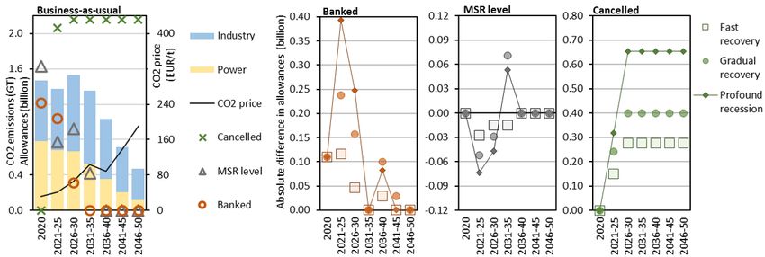
Imprint:

ifo Working Papers
Publisher and distributor: ifo Institute – Leibniz Institute for Economic Research at the
University of Munich
Poschingerstr. 5, 81679 Munich, Germany
Telephone +49(0)89 9224 0, Telefax +49(0)89 985369, email ifo@ifo.de
www.ifo.de

An electronic version of the paper may be downloaded from the ifo website:
www.ifo.de
ifo Working Paper No. 338

 MSR under Exogenous Shock: The Case of Covid-19 Pandemic

                                            Abstract

The EU implemented the Market Stability Reserve (MSR) in response to the 2008
financial crisis to deal with short-term impacts of future shocks, such as the Covid-19
pandemic. We link a model that intertemporally optimizes the handling of banked
allowances every five years with one that simulates the annual working of the EU
ETS including the MSR with its potential cancelling. Neglecting the pandemic,
2.16 billion allowances are cancelled. Accounting for the pandemic, 0.28 billion
additional allowances are cancelled if the European economy fully recovers by 2021,
which even overcompensates the 2020 drop in CO2 emissions. Additional cancelling
increases when the pandemic lasts longer, meaning that the MSR even outperforms
its initial purpose.

JEL code: C61, H23, Q41, Q51, Q54, Q58
Keywords: Covid-19 pandemic, EU ETS, Market Stability Reserve, decarbonization

             Valeriya Azarova*                                 Mathias Mier
    ifo Institute – Leibniz Institute for          ifo Institute – Leibniz Institute for
            Economic Research                              Economic Research
        at the University of Munich                    at the University of Munich
              Poschingerstr. 5                               Poschingerstr. 5
          81679 Munich, Germany                          81679 Munich, Germany
         Phone: +49-89-9224-1307                        Phone: +49-89-9224-1365
              azarova@ifo.de                                   mier@ifo.de

* Corresponding author.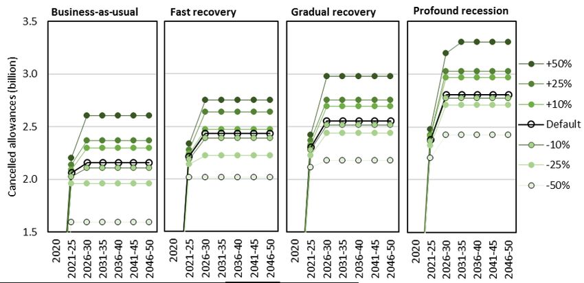
MSR Under Exogenous Shock: The Case of COVID-19 Pandemic
                                Valeriya Azarova1∗ , Mathias Mier        1

                 1   ifo Institute for Economic Research at the University of Munich

                            ∗ Corresponding   Author, E-mail: azarova@ifo.de

                                          September 2, 2020

                                                Abstract

         The EU implemented the Market Stability Reserve (MSR) in response to the 2008 financial
     crisis to deal with short-term impacts of future shocks, such as the COVID-19 pandemic. We
     link a model that intertemporally optimizes the handling of banked allowances every five years
     with one that simulates the annual working of the EU ETS including the MSR with its potential
     cancelling. Neglecting the pandemic, 2.16 billion allowances are cancelled. Accounting for the
     pandemic, 0.28 billion additional allowances are cancelled if the European economy fully recovers
     by 2021, which even overcompensates the 2020 drop in CO2 emissions. Additional cancelling
     increases when the pandemics lasts longer, meaning that the MSR even outperforms its initial
     purpose.

    Keywords: COVID-19 pandemic, EU ETS, Market Stability Reserve, Decarbonization

1    Introduction
The EU emission allowance (EUA) price dropped from 24.07 e/t to 15.25 e/t in March 2020 at
the start of the COVID-19 pandemic in Europe. This is not the first time that we observe such a
dramatic EUA price drop. The 2008 financial crisis caused an even higher price drop with a quite
similar reduction of economic activity [1]. Yet, in the aftermath of the 2008 financial crisis, the EUA
price remained below 10 e/t for over nine years even when the economic activity has already started
recovering [2]. In the case of COVID-19, however, the price recovered almost completely to 22.10 e/t
already in June 2020, just two months after the drastic drop.

                                                    1
One possible explanation for the difference in EUA price dynamics during the two crises might
be attributed to the legislative changes introduced in the EU Emission Trading System (ETS), for
instance, the establishing of the Market Stability Reserve (MSR). The MSR was established in 2015
and initially designed to reduce the short-term oversupply of allowances [3, 4]. The MSR was updated
in 2018 when, among other measures aiming to strengthen the EU ETS, a cancelling mechanism was
introduced: if the MSR level exceeds the auctioning volume, allowances exceeding the threshold
become permanently cancelled. According to [5] this new MSR rule can temporarily puncture the
waterbed effect of the EU ETS.1
       Contrary to [5] findings, other studies suggest that the introduction of cancelling (depending on
timeframe and firms’ price expectations) can create a green paradox such that cumulative emissions
increase in the long-term [7, 8, 9]. Concurrently, studies providing an overview of current research
efforts on EU ETS and its impact on carbon emissions and prices stress a lack of empirical and
simulation studies as well as absence of unanimity about its long-term functioning [10, 11, 12, 13].
       The discussions about the efficiency of the MSR are ongoing as the MSR began operating recently,
in January 2019, and will be reviewed in 2021. The COVID-19 pandemic represents an additional
challenge for the functioning of the EU ETS including the MSR [14, 15] because—since the beginning
of the COVID-19 pandemic—falling energy demand and CO2 emissions were reported [16, 17]. When
companies emit less CO2, they also need fewer allowances and may opt to sell their surplus so that
the total number of allowances in circulatation (TNAC) even increases.
       The MSR aims to “addresses the current surplus of allowances and improve the system’s resilience
to major shocks by adjusting the supply of allowances to be auctioned” 2 . The COVID-19 pandemic
represents such a major shock and will show whether or not the standard MSR mechanisms are robust
enough to handle the shock by balancing TNAC values and thus keep CO2 prices stable (and high).
       Using the intertemporally optimizing EU-REGEN model—a power market model with a module
to determine industrial CO2 emissions at five-yearly resolution—we calculate the short- and long-term
impacts of the COVID-19 pandemic via decreasing world market prices for fossil fuels (oil, natural
gas, coal), as well as declining industrial CO2 emissions and falling electricity consumption in Europe.
In particular, we determine CO2 emissions, EUA prices, the handling of banked allowances over time,
and resulting cancelling of allowances in the MSR by linking the EU-REGEN model to a simulation
model of the EU ETS at annual time resolution.
       We find that the MSR would cancel 2.16 billion allowances under pre-pandemic projections. This
   1
     The waterbed effect is defined as a situation when some emissions are abated, e.g., due to a supplementary policy
such as renewable support or phase-out of coal, but total emissions do not change due to the fixed emission cap [6].
   2
     See European Commission full text here https://ec.europa.eu/clima/policies/ets/reform_en#tab-0-0

                                                          2
number increases to 2.43 billion when the European economy recovers immediately in 2021 (called
fast recovery). Under a gradual recovery scenario, where the European economy remains below pre-
pandemic projections for five more years, cancelling increases to 2.56 billion. Highest cancelling
(2.81 billion) occurs in a profound recession scenario when the European economy is coping with the
consequences of the COVID-19 until 2050. While our results demonstrate that MSR is effective in
dealing with the exogenous shock of COVID-19, we also find that its performance is sensitive to policy
context and other adjustments, for instance, the introduction of higher wind turbines from 2036-40,
which can fundamentally change the dynamics of the MSR.
We present the background of the COVID-19 pandemic in Section 2, and Section 3 shows the
derived scenarios for the future development of European economies in the aftermath of the exogenous
shock trigger by the COVID-19. Section 4 presents the methods by introducing modelling techniques
and assumptions. Section 5 presents results with regard to MSR and power generation mix. Section
6 checks robustness of our results with respect to MSR and, in particular, cancelling results. Section
7 concludes.
2 COVID-19 pandemic
On December 31, 2019, Chinese authorities acknowledged that the first COVID-19 infections occurred
in Wuhan (Hubei province, China) by reporting an accumulation of pneumonia cases of unknown
origin. Media traced back the earliest infection to a 55 years old man on November 17, 2020, almost six
weeks before Chinese authorities acknowledged that a novel virus causes the severe acute respiratory
syndrome Coronavirus 2 (SARS-CoV-2).3
Massive and very stringent shutdowns of industries all over China and lockdowns of people in their
homes stopped the non-controlled spreading outside from the origin in Wuhan to the rest of China
[18]. The COVID-19 pandemic had its major (economic and health) impact in China in January and
February 2020. Industry production decreased by 13.5% [19] and more than 4,500 people died due to
COVID-19 infections, most of them in Wuhan. However, global economic growth and, in particular,
stock indices such as the Dow Jones or Euro Stoxx 50 remained stable showing no signs of impact of
the COVID-19. Same was observed for world market prices of crude oil, natural gas, and hard coal.
In March 2020, China already started to lift quarantine measures and industry production in-
creased again, but Europe and the United States became the two new global epicenters of the pan-
demic and first economic damages became evident. Moreover, Western countries seemed to struggle
3
See https://www.scmp.com/news/china/society/article/3074991/coronavirus-chinas-first-confirmed-covid-19-case-
traced-back for the original article.
3more to contain COVID-19, because human rights and constitutional laws make it difficult to act as
strict as in China.4
The COVID-19 pandemic began to severely affect the world economy from the beginning of March,
when Italy shut down major industries and stopped public life due to viral spreading of COVID-19
infections. Other countries in Europe followed the example of Italy, but the spreading of the virus
could not be stopped, so that also the United States and almost every country on the globe experienced
a rapidly increasing number of infections, followed by further and more severe shutdowns of industries
and a reduction of public life to contain further spreading.
The pandemic also affected stock and commodity markets, in particular, the price for oil dropped
heavily. Political disagreement even fostered this development in the beginning. During a meeting at
the Organisation of the Petroleum Exporting Countries (OPEC) in Vienna on March 6, 2020, a refusal
by Russia to slash oil production triggered Saudi Arabia to retaliate with extraordinary discounts to
buyers and a threat to pump more crude oil. Saudi Arabia, regarded as the de facto leader of the
OPEC, increased its provision of oil by a quarter in March (compared to February) 2020—taking the
production volume to an unprecedented level. This caused the steepest one-day price crash seen in
nearly 30 years. On March 23, 2020, Brent Crude Oil dropped by 24% to $34/barrel to stand at $25.7.
Although a slowdown in the number of COVID-19-related deaths has caused some stabilization of oil
prices, on April 20, 2020, the Brent price dropped to $15.98/barrel, while the West Texas Intermediate
traded at the New York stock exchange even turned negative due to completely filled storages. The
pandemic also impacted other related commodity prices such as natural gas, but also hard coal prices
dropped (although to a lesser extent).
From April, 2020, onward, the pandemic is the (only) dominating topic in world’s media, science,
as well as political meetings and decision making on all governmental levels. While the short-term
effects of the crisis can already be observed and effective shutdown-lockdown-measures stabilized
infection rates, the long-lasting economic impacts are still unclear but expected to be severe. Addi-
tionally, the predictions are the major driver for political decisions with regard to lifting quarantines
and reboot industries as well as services again (as seen in China, Italy, Spain, Germany, United States,
and many other countries) to limit the long-run impacts of the crises to a digestible level. In this
regard, our analysis provides some guidelines for political decision making with regard to European
climate policy by developing three scenarios that reflect possible long-run impact of the COVID-19
pandemic in the next section.
4
Complete lockdowns of people (belonging to risk groups) are hard to justify by Western constitutions, and also
data protection laws, especially in Europe, make it difficult to track infected people via mobile phones as South Korea
did quite successfully.
43 Scenarios
COVID-19 broke global supply and demand chains, and is considered one of the major global dis-
ruptions over the last century [20, 21]. The spread of the virus and related measures introduced by
governments worldwide, including various models of shutdowns, lockdowns, and quarantines, have
interrupted global trade, depressed asset prices, and forced companies to put their activities on hold
or shut them down completely. In the long run, this crisis might trigger a reaction similar or even
more severe to the one observed during the 2008 financial crisis on global markets [22, 16, 15, 23].
However, unlike the financial crisis, the COVID-19 shock is exogenously given and a fast “V-shaped”
recovery of the economy is not a realm of fantasy.
We differentiate between short- and long-run impacts of the COVID-19 pandemic. Short-run im-
pacts result directly from the shutdown of industries, commerce, and services, as well as the lockdown
of people to reduce public life and enhance social distancing. We limit the short-run impacts to 2020:
January remains unaffected by the exogenous shock of the pandemic. The next seven months (until
the end of August) are impacted most due to different levels of (recurring) shutdowns and lockdowns.
For example, commodity prices drop from 16% (coal) up to 66% (oil), electricity demand by 10%,
and industrial CO2 emissions by 20% in April 2020. We project that the shutdowns and lockdowns
are successively lifted until the end of 2020. Prices recover (oil price drop is 5% at the end of 2020)
and also electricity demand and industrial CO2 emissions increase again to 95% of its pre-pandemic
projection (see Table 1 for details).
From 2020 onward, we suggest that the long-run impacts can develop in different directions.
Similar projections are made by [24], who suggest that the earliest we can expect the pandemic to
be over is by 2021, while in the worst case scenario we might be still coping with the impacts until
2025. We distinguish between three scenarios that reflect the potential impact of the pandemic on
economic growth (i.e., industrial CO2 emissions), commodity prices (crude oil, natural gas, and hard
coal), and electricity demand:
• “Fast recovery” foresees a rapid return to pre-pandemic projections by March 2021.
• “Gradual recovery” expects that the number of new infections will slow down, but quarantines
and social distancing measures will stay in place due to regulations, absence of a vaccine, or
new waves of the virus. Hence, there is no “V-shaped” recovery of the economy, but a step-wise
process with a return to pre-pandemic levels by 2026.
• “Profound recession” suggests a strong long-term impact on European (and global) supply
chains, and a drop in industrial CO2 emissions and electricity consumption that persists until
52050.
Where the first two scenarios are motivated and supported by published studies [24, 25] and are based
on projections of the length of confinement measures, profound recession is motivated by the un-
precedented socio-economic impact of COVID-19. This impact is already observable and might cause
significant changes in behaviors and lifestyles such as higher acceptance for home office, decreased
mobility, and lower consumption of goods and services. Tables 1 and 2 summarize the quantitative
assumptions. The following three Subsections contain the underlying motivation.
Table 1: Scenario assumptions for the short-term impacts of the COVID-19 pandemic
Jan 20 Feb 20 Mar 20 Apr 20 Mai 20 Jun 20 Jul 20 Aug 20 Sep 20 Oct 20 Nov 20 Dec 20 2020
Oil price 1.00 0.86 0.53 0.34 0.47 0.62 0.67 0.73 0.78 0.84 0.89 0.95 0.72
Natural gas price 1.00 0.92 0.92 0.87 0.90 0.89 0.91 0.92 0.94 0.95 0.97 0.98 0.93
Coal price 1.00 0.99 0.95 0.84 0.79 0.81 0.84 0.86 0.89 0.92 0.95 0.97 0.90
Industrial emissions 1.00 1.00 0.90 0.80 0.80 0.85 0.85 0.85 0.90 0.90 0.95 0.95 0.90
Electricity demand 1.00 1.00 0.95 0.90 0.90 0.93 0.93 0.93 0.95 0.95 0.95 0.95 0.94
Short-term impacts (2020) are the same across all the three scenarios.
Data on commodity price changes are sourced from Trading Economics until June 2020, for subsequent periods own assumptions
were made.
Table 2: Scenario assumptions for the long-term impacts of the COVID-19 pandemic
2021-25 2026-50
Fast recovery Gradual recovery Profound recession Fast recovery Gradual recovery Profound recession
Oil price 1.00 0.98 0.98 1.00 1.00 1.00
Natural gas price 1.00 1.00 1.00 1.00 1.00 1.00
Coal price 1.00 1.00 1.00 1.00 1.00 1.00
Industrial emissions 1.00 0.98 0.95 1.00 1.00 0.95
Electricity demand 1.00 0.98 0.95 1.00 1.00 0.95
The assumptions are made relative to BAU level of the respective parameter, with 1.00 meaning the BAU value.
3.1 “Fast Recovery ” Scenario
Unlike the financial crisis of 2008—whose impact on the world economy lasted several years [26, 27]—or
the Great Depression era—which lasted much of the 1930s [28]—the crisis triggered by the COVID-19
pandemic as well as the induced plunge in global consumption in general and electricity demand in
particular are primed to recover once the pandemic fades and lockdown and quarantine measures
are lifted. The underlying projection is that the demand decrease for many households (e.g., for
restaurants, travelling, and shopping) is not triggered by loss of purchasing power but by lockdown
measures [29].
The key difference of the current situation to the 2008 financial crisis (or the Great Depression) is
the exogeneity of the pandemic shock. Former crisis had their origins in excessive and artificial (not
based on actual value) growth and asset bubbles. This fact makes a fast recovery scenario plausible.
6Additionally, governments launched unprecedented critical support to bring the economies back on
track, which was not the case during the Great Depression. Also support programs, launched in the
aftermath of the 2008 financial crisis, were far beyond the scale of current ones. For instance, the
EU announced a e1.7 trillion rescue package in an attempt to mitigate the economic impacts of the
pandemic with contributions from all member states and European countries that are not part of
the EU (e.g., United Kingdom and Switzerland) [30]. Considering the above-mentioned aspects, we
assume that a swift recovery scenario with a “V-shaped” return to a pre-pandemic world economy
status is possible. Also the race for treatments and vaccines can contribute to actual realization
of this scenario. We thus assume a fast return to the business-as-usual (BAU) after the shutdown
and lockdown measures are lifted: industrial CO2 emissions as well as electricity demand is back at
pre-pandemic level from 2021 onward. The same holds for commodity prices (oil, natural gas, and
coal).
3.2 “Gradual Recovery ” Scenario
This scenario is supported by the fact that there is still no (well-tested) vaccine available, and no
solution for the pandemic except to be contained gradually. Additionally, recent projections [24]
using a set of viral, environmental, and immunologic factors to estimate the dynamics of the current
pandemic, include a scenario where the COVID-19 pandemic requires a persistent degree of social
distancing or intermittent lockdowns until 2025. Furthermore, even countries which were hit less
severely by COVID-19 and already announced an ease of lockdown measures, like Austria, plan for
months of step-by-step return to before-COVID-19 times. The danger of returning to more stringent
measures again places major industry players on hold. This uncertainty will last for at least several
months. We thus assume that there is no “V-shaped” recovery and the world economy will be coping
with the consequences of the pandemic until 2025. In particular, we assume that a lower level of
electricity demand will remain persistent over the course of the five years after the start of COVID-19
driven crisis.
3.3 “Profound Recession” Scenario
COVID-19 has a strong socio-economic impact on all the sectors including agriculture and manufac-
turing (shortage of manpower, inability to work from home, supply chain disruptions), power (drop
in demand, plunge of oil price) and also an unprecedented impact on education (school and univer-
sity closures) as well as even research (redirection of financing towards COVID-19 research, cancelled
conferences and workshops). Thus, this crisis has already created profound political and social un-
7certainty which boosts the scale of the pandemic. It is also worth mentioning the difficulty predicting
the end of the current crisis, as no scientifically-sound data on the duration of lockdowns, possibilities
of second and third waves, and successful development of vaccines (which are now being elaborated)
are available. All these factors increase the uncertainty in which today’s economic decisions are made.
Especially, looking at current situation in the United States, where lockdowns triggered the highest
level of unemployment since the Great Depression and business failures [31]. Even after an economic
restart, the damage to businesses and debt markets might last even longer than after the 2008 finan-
cial crisis, especially when considering that global debt was already at record-breaking levels before
the pandemic starts.
Another motivation for this scenario is rooted in the expected behavioral change triggered by the
exogenous shock of the pandemic and introduced lockdown measures [32]. Companies in technology,
financial, insurance branches, and other industries that can successfully function remotely are choosing
to keep their employees home longer. For instance, Facebook announced that its employees are allowed
to work from home at least until the end of 2020. Risk groups (older population as well as people with
health preconditions) and households with children under 15 years will be restricted to work from
home for a longer period of time. This situation can cause a behavioral shift in terms of home office
work becoming a common practice, leading to changes in CO2 emissions due to decreased commutes,
as well as more efficient and reduced power demand. Additionally, previous studies analysing changes
in consumers’ behaviour in post-financial crisis time show that, in the following years, consumers
demonstrate increased social responsibility in their consumption patterns as well as decreased wasting.
These dynamics could also trigger more efficient energy demand and electricity consumption in post-
pandemic times [33]. We thus assume that the drop in electricity demand by 5% at the beginning of
2021 remains persistent until 2050.
4 Methods
4.1 EU-REGEN Model
The EU-REGEN model is a dynamic partial equilibrium model of the European power market (see
[34] for the underlying dynamics and [35] as well as [36] for applications). The model optimizes
dispatch, decommissioning, and investments (generation, storage, and transmission capacity) from an
investor’s perspective intertemporally until 2050. 2019 (as calibration year) and 2020 (as pandemic
year) are modelled as single years, which allows us to calibrate a pre-pandemic starting point or fully
capture the short-run impacts of the pandemic, respectively. All succeeding periods cover five years.
8The model includes 16 different generation technologies. Each technology is further distinguished
into vintages blocks to account for different characteristics of power plants of the same type (but
different age) or varying resource quality of intermittent renewables. The model groups 28 countries
(EU27 excluding Malta and Cyprus, including Norway, Switzerland, and United Kingdom) into 12
regions that are connected via transmission lines. The model chooses and weights 100 hours (number
is endogenous) from the 8,760 hours of the year to minimize the error to the real extremes of wind,
solar, and load in all regions. CO2 emissions from the electricity sector are calculated in detail by
using average emission factors of carbon-containing fuels (oil, coal, lignite, and natural gas; bioenergy
is assumed as zero-emission-fuel) and conversion efficiencies of technologies subject to exogenous
technological change. The model allows for carbon capture and storage (CCS) in combination of coal
(Coal-CCS), gas power (Gas-CCS), and bioenergy (Bio-CCS, negative CO2 emissions).
4.2 Exogenous Shock and Investment Behavior
The COVID-19 pandemic is an exogenous shock with no impact in 2019 (investors could not foresee
the occurrence of the pandemic) and the most direct impact in 2020. Investments from a model
specification that neglects the impact of the pandemic (the business-as-usual, BAU) creates a pre-
pandemic benchmark for planned investments. We then fix investments in 2020 and define upper
bounds for investments in periods 2021-25 (for all technologies except wind turbines and solar tech-
nologies) and 2026-30 (for coal, lignite, and nuclear power plants). Investors are still able to decide to
stop a planned investment (at full sunk cost), and to decommission capacity that is already in place.
4.3 EU ETS
The EU ETS followed from the 1997 Kyoto agreement and started in 2005 with the first trading
period (until 2007). We are currently at the end of the third trading period (2013 to 2020) and close
to start the fourth trading period in 2021 (until 2030). Free allocation of allowances and the impact
of the 2008 financial crisis yield structural and persistent carrying of tradable allowances to the next
trading periods via banking. The downturn in economic activity due to 2008 financial crisis and the
related fostering of investments in energy efficiency as result of the past stimulus packages reduced
carbon emissions [1]. Resulting prices were perceived as too low to incentivize substantial investments
into carbon-neutral technologies, whereas the possibility of banking even kept them positive.
The EU reacted with backloading of 0.9 billion allowances from 2014 to 2016 and the implemen-
tation of the Market Stability Reserve (MSR) [12, 3, 4]. The backloading is moved to the MSR in
2019, and, from 2019 to 2023 (from 2024 onward), 24% (12%) of the previous year’s total number of
9allowances in circulation (TNAC) will be deducted from next years auctioning volume and transferred
in the MSR when the previous year’s excess is above 0.833 billion allowances.5 At the end of 2018
(2019), TNAC was 1.66 (1.39) billion allowances, leading to a movement of allowances in the MSR
and reduction of planned auctioning of 0.4 (0.33) billion in 2019 (2020). Allowances will be taken out
of the MSR and reinserted into the market via auctioning (0.2 billion before 2023, 0.1 billion from
2024 onward) when the excess is below 0.4 billion allowances. Additionally, allowances in the MSR
will be cancelled permanently when their level exceeds the threshold of previous year’s auctioned
allowances.6
4.4 EU ETS Assumptions
We cannot precisely forecast the planned supply and the auctioning volume of allowances—that is,
how many allowances are planned to get allocated and auctioned each year—due to the various legal
possibilities of each participating country to increase and decrease the absolute amount of supplied
allowances (allocated and auctioned) and the share of auctioned allowances. Also the structure of the
EU ETS with regard to trading periods after 2030 is unclear.
Planned supply. In 2019 (2020), planned supply (without MSR inflow) is at 1.69 (1.63) billion
allowances, whereas the 2019 (2020) cap is at 1.86 (1.82) billion; meaning that the legal emission cap
is not of major interest to determine planned supply. For example, the Coalexit enables the German
government to reduce the number of supplied allowances. We, therefore, assume that less allowances
(than the legal cap) will be supplied to the market from 2021 to 2025, and linearly interpolate between
2020 supply (1.63 billion) and 2026 cap (1.53 billion) to determine planned supply in the years in
between. From 2026 onward, the planned supply equals the cap. Also the role of the Brexit (and the
related adjustments of the cap as well as supply) remains unclear. For parsimony, we assume that the
United Kingdom binds their emissions to those of the EU ETS development (or sets a carbon price
similar to the resulting EUA price).
Planned auctioning. Planned auctioning in 2014 (2015, 2016) was 1.02 (0.93, 0.92) billion, but
true auctioning was 0.62 (0.63, 0.72) billion lower due to the backloading. In 2017 and 2018, planned
and true auctioning were at the same level. In 2019, the MSR started operating and deducted 0.4
billion allowances from the planned auctioning volume of 1 billion. As a consequence, the share
5
The excess is the annual difference between (aggregated) supply and (aggregated) demand. Subtracting the total
MSR holdings yields TNAC.
6
Note that the auctioning volume is endogenous subject to MSR inflow/outflow.
10of auctioned allowances (from total supply) is endogenous to the working of the MSR. 0.66 billion
allowances will get auctioned and 0.33 billion allowances are deducted from the auctioned volume
in 2020 due to the MSR. The planned auctioning of 0.99 billion presents a share of 61% from total
planned supply (1.69 billion). The participating countries committed themselves to increase the share
of auctioned allowances over time but no details have been fixed yet. We thus assume that the share
of auctioned allowances increases linearly from 61% in 2020 to 100% in 2050.
Trading periods. The fourth trading period starts in 2021 and lasts until 2030. We split the
trading period in two parts as done by the legal framework for organisational reasons. We further
assume that trading periods from 2031 onward will also last five years (which fits the model periods).
Excess from 2020 (2025, 2030, ...) is available via banking in years 2021 (2026, ..., 2046) to 2025
(2030, ..., 2050).
4.5 Model Linking
A simulation model determines—under given demand for allowances—each year’s (1) planned supply,
(2) allowances moved to/from the MSR, and (3) related cancelling. Deducting MSR movements from
planned supply leads to true supply of allowances. The EU-REGEN model endogenizes—subject to
the planned supply, MSR movements, and MSR cancelling from the simulation model—each period’s
(4) demand for allowances by determining CO2 emissions, and thus the (5) banking decision of
intertemporal optimizing (perfectly competitive) investors. The shadow price of the carbon market
constraint is used to calculate the resulting EUA price.
We start with disabling the MSR and potential cancelling in the simulation model and feed
the optimization model to obtain an unbiased starting point for the iterations. We then start the
iterative process. First, we activate MSR inflow/outflow and conduct iteration runs until results of the
simulation model match those of the optimization model. Next, we also activate potential cancelling
and repeat the prior process.7 This allows us to be robust against the selection of starting points
when calculating the different scenarios.8 Remember from Tables 1 and 2 that industrial emissions for
the three scenarios under consideration are pre-defined in relation to BAU results. We thus finalize
the iterative process for BAU first and then fix industrial emissions in the three scenarios based on
BAU emissions and subject to the scenario assumptions.
7
We need one run to obtain the starting point, around 5 runs for the first iteration step, and a maximum of 10 runs
for the second iteration step.
8
We use this process in the sensitivity analysis in Section 6 as well. However, calculating just the BAU scenario in
that way and use the BAU results as starting point for the scenarios (MSR flows and cancelling are activated) leads to
the same results.
114.6 Industrial CO2 Emissions
The EU ETS covers electricity generation, other (mainly energy-intensive) sectors, and aviation. We
abstract from aviation (and related supplied allowances) and group all EU ETS sectors except the
power sector into one industry sector. Power and industry sectors emitted 0.97 (0.84) Gt or 0.71 (0.72)
Gt CO2 in 2018 (2019), respectively. The EU-REGEN model is not capable of calculating industrial
CO2 emissions in such a detail as emissions from electricity generation. Instead, we calibrate the
emission abatement of the industrial sectors, to the best of our knowledge, by assuming that the
relation of those sectors’ emissions to those of the power sector changes from 0.85 in 2019 to 3.06 in
the period 2046 to 2050 (see Table 3). This relation is based on a scenario of the 4NEMO project—
that uses a CGE model for the calculation of different scenarios (of EU climate policies) to calibrate
European power market models. The CGE model predicts average power sector emissions of 0.15 Gt
(industry emissions of 0.46 Gt) in 2046-50 and a resulting CO2 price of 176 e/t. We calculate (in the
BAU) power sector emissions of 0.12 Gt (industry emissions of 0.36 Gt) at a CO2 price of 191 e/t,
which is—from our perspective—sufficiently close to the CGE outcome.9
Table 3: Assumptions about the ratio of industrial CO2 emissions to those of the power sector under
BAU
2013 2014 2015 2016 2017 2018 2019 2020 2021-25 2026-30 2031-35 2036-40 2041-45 2046-50
0.6 0.65 0.65 0.67 0.69 0.73 0.85 0.88 1.01 1.29 1.58 1.93 2.51 3.06
Values until 2019 indicate real world observations. Values from 2020 to 2046-50 indicate CGE model results.
These assumptions reflect that the power sector has (in general) lower abatement cost than the
industry sector, and thus higher relative abatement. However, the power sector still sets the price
due to the variety (and level of usage) of different technologies applicable for emission abatement.
Wind and solar technologies have quite low abatement cost when the share of wind and solar in
total generation is still low. The abatement cost of wind and solar technologies rises with their share
increasing in the generation mix, and also when high quality wind and solar sites become scarce. Fuel
switching from coal to natural gas also offers abatement at quite low costs[37]. Finally, multiple CCS
and different storage technologies (short-term storages such as batteries and long-term storages such
as power-to-gas technologies) in combination with intermittent renewables such as wind and solar are
perceived to have the highest abatement cost.
9
The calibration databases are available upon request and their (open access) publishing is in process.
125 Results
We model the EU ETS by iteratively matching results of the optimization model EU-REGEN (uses
2019 as calibration year and optimizes periods 2020, 2021 to 2025, ..., 2046 to 2050 intertemporally)
to those of the simulation model of the EU ETS (2008 to 2019 as calibration years and simulation
of 2020 to 2050). Although the EU aims to reach carbon neutrality by 2050 (Green Deal ), we stick
with the current legislative structure (and related goals) of the EU ETS and keep the linear reduction
factor of 48 million from 2021 onward, leading to a cap of 0.38 billion in 2050.10
Figures 1 and 2 present our main results. 2020 is depicted as single year and all succeeding years
are grouped into 5-year-intervals. The simulation model of the EU ETS provides annual values. We
will feed our results, whenever useful, by the knowledge of them. Pre-pandemic projections (business-
as-usual, BAU) are shown on the very left side of the figures, whereas the remaining space is dedicated
to the pandemic scenarios.
5.1 Implications for EU ETS and MSR
The left part of Figure 1 shows carbon emissions, the functioning of the MSR, the usage of the “bank”
(all left axis), and resulting CO2 (allowance) prices (right axis). Average emissions (over the respective
period) of the power sector are shown by yellow bars, emissions of remaining EU ETS sectors (except
aviation) are pooled as industry in the blue bars, so that the stack shows total emissions without the
impact of the pandemic. The working of the MSR is depicted by the cancelling of allowances in the
MSR (green saltires) and the resulting MSR level (grey triangles). Red loops present the banking
decision and the black solid line the resulting CO2 price.
Total emissions decrease from 1.56 Gt in 2020 to 0.47 Gt in the period 2046-50, a reduction of 77%
to 2005 emissions. At the same time, the CO2 price rises from 31 EUR/t in 2020 to 191 EUR/t. Power
sector emissions decrease from 0.78 Gt in 2020 to 0.12 Gt in 2050 (reduction of 85%). Conversely,
industrial CO2 emissions increase—due to the assumptions about the ratio between industrial CO2
emissions and those of the power sector (see Subsection 4.6)—from 0.69 in 2020 to 0.86 Gt in 2026-30
(and then successively drop to 0.36 Gt in 2050), so that total emissions have a mid peak at 1.53 Gt
in 2026-30.
At the end of 2019, 1.39 billion allowances were sold but unused (total number of allowances in
circulation, TNAC). Banked presents the intertemporal optimized handling of these allowances. 0.17
billion allowances from this “bank” are used in 2020. Firms successively empty the bank until it
10
Section 6 tests robustness of our findings with regard to a changed in the legislative structure of the EU ETS
according to the Green Deal.
13Figure 1: CO2 emissions, prices, banked allowances, and the MSR
The very left part shows the BAU and the other parts show absolute differences in banked allowances (red), the MSR level (grey), and cumulative
MSR cancelling (green) for fast recovery (squares), gradual recovery (circles), and profound recession (rhombus). Cancelled shows cumulative
values. MSR level and Banked show the respective values at the end of each period.
clears at the end of 2031-35. In the following periods, CO2 emissions match exactly the supply of
allowances.
In 2020, 0.33 billion allowances are moved into the MSR, resulting in an MSR level of 1.63 billion
allowances (1.3 billion allowances are already moved into the MSR in 2019, see Subsection 4.3 for
details). Additional allowances are moved into the MSR in 2021-25 (1.21 billion) and 2026-30 (0.24
billion). From 2030 onward, allowances are moved out of the MSR (0.1 billion each year) until it is
completely cleared by the end of 2036-40. Observe that the MSR level drops in 2021-25—although
allowances are still moved into the MSR—due to the cancelling mechanism. 1.72 billion allowances
are cancelled in 2023 and 0.24 (0.11) billion in 2024 (2025). Cancelling allows occurs in 2026 and 2027
(0.09 billion in total) because movements into the MSR (until 2026) increase the MSR level above
the cancelling threshold of previous year auctioned allowances.
The cancelling leads to an increase in the CO2 price in 2021-2025, which continues through the
following two periods up to 103 EUR/t in 2031-35. A small drop in the CO2 price development in
2036-40 (to 88 EUR/t), complemented by a 24% drop in total emissions (from 1.36 to 1.04 Gt) could
be explained by an exogenous technology boost that allows wind turbines up to 140 metres high. As a
result, investors do not use the total bank in the very last periods (with highest prices), but massively
in the periods prior to this technology boost (0.18 billion in 2021-2025, 0.72 billion in 2026-30, and
0.32 billion in 2031-2035).
Looking at the impact of the COVID-19 pandemic, we find similar banking patterns for all three
scenarios, although the amplitudes tend to be higher for gradual recovery and profound recession.
14The bank clears in all three scenarios at the end of 2031-35 (as it does in BAU). However, in all three
scenarios the bank fills up slightly in 2036-40 due to the introduction of the technology boost.
Considering the MSR level in all three scenarios, the MSR level is below BAU in 2021-25 and
2026-30, whereas the difference is highest for profound recession and lowest for fast recovery (. note
that the MSR level changes with one year delay (see Subsection 4.3), so that BAU and all scenarios
have the same 2020 value). The lower MSR level does not hamper the magnitude of cancelling due to
the dynamics of the MSR: movements into the MSR reduce next years auctioning volume and thus
increase the tendency to cancel allowances because the cancelling threshold drops with auctioned
allowances. This cancelling dynamic reinforces when allowances are placed into the MSR in two
succeeding periods.
Evaluating the climate impact of the MSR, 0.28 (0.4, 0.65) billion additional allowances are
cancelled, whereas the 2020 drop in emissions is 0.11 billion. Meaning that the initial drop is (more
than) fully compensated in fast recovery by additional cancelling which can be interpreted as a positive
climate impact of the MSR. Additionally, persistent lower emissions in gradual recovery and profound
recession indeed reinforce cancelling.
5.2 Implications for Generation Mix
We now briefly discuss the impact on the European electricity generation mix. Observe from the left
side of Figure 2 that lignite and coal almost completely drop out from 2026-2030 onward under the
BAU projection. Wind, solar, and Gas-CCS accomplish the major part of decarbonizing the system.
Interestingly, already in the period 2026-30 (2031-35) Gas-CCS takes a minor (major) share in the
generation mix at a CO2 price of 66 (103) EUR/t. Bio-CCS becomes active in 2041-45 (at CO2 price
of 137 EUR/t), but its absolute contribution remains small due to regional biomass limits.
Looking at the right side of Figure 2, 2020 generation drops due to lower electricity demand (-6%).
Further more, the clean technologies gas and bioenergy—as marginal generation technologies—suffer
most from the short-term impact of the pandemic. 2020 production of gas decreases by 24%, while
production of bioenergy drops by 81% (lignite only by 3%). Coal production even increases by 15%.
In fast and gradual recovery, these differences dissipate in 2021-25. Turning to the generation
mix of profound recession, we do not observe full convergence to the BAU projections because the
electricity demand drop of 5% persists until 2050. We find in the scenario less lignite, coal, gas, wind,
and nuclear generation in 2021-25. Additionally, Gas-CCS, wind, and solar technologies are those
that suffer most as marginal generation sources, while gas production even increases from 2026-30
onward due to structurally lower carbon prices.
15Figure 2: Generation mix
The very left part shows the BAU and the other parts represent the differences of the scenarios to the BAU. The relative difference is the ratio of
the absolute difference in generation from a technology to total generation from the BAU.
6 Sensitivity Analysis
Three crucial assumptions determine the level of cancelling and the dynamics of the MSR: (1) higher
wind turbines from the period 2036-40 onward (called technology boost), (2) evolution of the EU ETS
allowance cap, and (3) the ratio of industrial emissions to those of the power sector.
6.1 No Technology Boost
Higher wind turbines can be installed in the default calibration from the period 2036-40 onward;
resulting in profiles with higher full-load hours for wind on- and offshore capacity that is installed
from 2036-40 onward. In Figure 1 due to this assumption a decrease in the carbon price in 2036-40 due
to the expansion of wind onshore generation (see Figure 2) is observed. We now neglect the impact
of the technology boost by using the same wind profiles as used for wind capacity that is installed
in the periods before. Carbon prices reach 224 EUR/t (+18%) in 2050 (under BAU projections, 214
EUR/t in fast and gradual recovery, 198 EUR/t in profound recession) due to lower generation from
wind onshore and resulting increased usage of Gas-CCS.
The whole dynamics of banking and cancelling change. In the first two periods, bank usage is
higher without technology boost, so that the bank clears already at the end of 2026-30 period. This
development is accompanied by overall higher emissions until 2026-30, and overall lower emissions in
periods 2031-35 (1.29 vs. 1.36 Gt) and 2036-40 (0.96 vs. 1.04 Gt). From 2041-45 onward, emissions
with and without boost are the same. Higher emissions in period until 2026-30 lead to lower TNAC
16values and thus less movement of allowances into the MSR. For example, 0.47 billion allowances
are moved into the MSR in 2021-25 without boost but 1.21 billion with technology boost. In total,
cancelling is 40% lower (1.29 vs. 2.16 billion) if the possibility of higher wind turbines introduction
is neglected in our model. The technology boost leads to withholding of banked allowances and
investments into wind onshore. In particular, the limited potential of high-quality wind sites leads
to postponement of investments into the period where higher wind turbines are available to populate
the high-quality sites with the higher turbines. Without technology boost, those strategic actions are
not relevant and the bank clears straightaway.
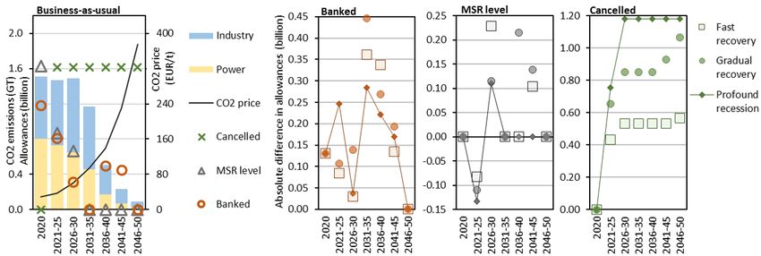
Figure 3: EU ETS and MSR without technology boost
Looking at the COVID-19 impacts, we find that the differences in banked allowances and MSR
levels are similar to the those of the specification with technology boost. Yet, cancelling under
profound recession is now almost the same as the cancelling in gradual recovery. This result underlines
the fickleness in general and the impact of the reinforced cancelling mechanism in particular. As stated
in Subsection 4.3 24% ( 12% from 2024 onward) of the TNAC are moved into the MSR and deducted
from next year’s planned auctioning volume. The cancelling then refers to the realized auctioning
volume after MSR inflow or outflow respectively. Thus, when allowances are moved into the MSR,
next year’s cancelling threshold drops thereby increasing the likelihood of cancelling. This reinforcing
cycle of MSR inflows and cancelling occurs when considering the technology boost under profound
recession.11 On contrary, shifting into the MSR is not sufficiently high to reach the cancelling threshold
without the technology boost.
11
Note that the reinforcing cycle turns to no cancelling (instead of higher cancelling) under MSR outflow because
next year’s auctioning volume and thus the cancelling threshold rises.
176.2 Green Deal
We use the current legislative structure of the EU ETS to analyze the impact of the COVID-19
pandemic on the long-term functioning of the MSR. However, the EU Commission is actively working
on reforms of the EU ETS under the synonym Green Deal [38]. The Green Deal presents aspirations
to reach carbon neutrality (including offsets and carbon sinks as well as futuristic technologies) in
the EU in 2050. We consider carbon neutrality within the EU ETS as a pre-condition to reach this
target. We thus change the linear reduction factor in 2026 from 48 to 75 million, so that no new
allowances are supplied to the market from 2046 onwards. Banked allowances and MSR holdings can
still be used until 2050. We further keep the MSR inflow rate at 24% and the outflow at 200 million
from 2024 onward to avoid persistent cancelling when the MSR cannot clear fast enough in response
to a reduction of supplied allowances.12
The results are given in Figure 4 and demonstrate that under the Green Deal specification the
CO2 price rises up to 376 EUR/t in 2050 because power sector emissions drop from 115 to 22 Gt
(industry emissions from 355 to 68 Gt). Firms increase emissions until 2021-25 (as they do without
technology boost), but start investing into clean technologies (Gas-CCS generation is almost five
times higher in 2026-30) as soon as the cap tightens from 2026 onward. Under default assumptions,
the bank clears in the period 2031-35. In case of Green Deal, the bank clears as well in 2031-35, but
then fills up again in the two succeeding periods and is used in the very last period where no new
allowances are supplied to the market anymore.
Figure 4: EU ETS and MSR under Green Deal
12
The assumption about the share of auctioned allowances (see Subsection 4.4 remains unchanged.
18The higher emissions (and lower banking) in the first two periods fundamentally reduce the level
of cancelling (1.61 vs. 2.16 Gt, -25%). This difference is less pronounced when taking into account
the impact of COVID-19. For instance, in fast recovery scenario, the cancelling is 10% lower (2.2
vs. 2.4 Gt). Yet, the opposite effect is observed under gradual recovery with the cancelling higher
by 5% (2.68 vs. 2.56 Gt). In profound recession scenario the differences in level of cancelling with
and without the Green Deal are insignificant and can be neglected (2.79 vs. 2.81 Gt). The results
of this analysis again underline the sensitivity of the MSR to a slightly changing environment and
assumptions. The pandemic impacts reduce the emissions in 2020, which is a crucial point with regard
to 2023 initial cancelling. The possibilities to react until initial cancelling are limited, and we even
calculate a cancelling rebound effect under gradual recovery. However, our results are robust with
regard to the qualitative impact of COVID-19 scenarios compared to pre-pandemic projections.
6.3 Industrial CO2 Emissions
In order to show the robustness of our results with respect to the assumption of the ratio between
industrial CO2 emissions and those of the power market, we model six additional ratios (-50%, -25%,
-10%, +10%, +25%, +50%), which are presented in Table 4. Lower ratios represent better abilities
of the industrial sector (other EU ETS sectors, excluding power generation and aviation) to reduce
carbon emissions. Higher ratios in turn imply higher abatement cost.
Table 4: Sensitivity analysis assumptions: ratio of industry to power sector CO2 emissions
2020 2021-25 2026-30 2031-35 2036-40 2041-45 2046-50
-50% 0.87 0.95 1.11 1.22 1.34 1.53 1.63
-25% 0.87 0.98 1.20 1.40 1.63 2.01 2.33
-10% 0.88 1.00 1.26 1.50 1.81 2.30 2.75
+10% 0.88 1.03 1.34 1.64 2.04 2.68 3.31
+25% 0.89 1.04 1.39 1.75 2.22 2.97 3.74
+50% 0.90 1.08 1.48 1.93 2.51 3.44 4.44
The percentage change refers to the differences in the 2050 ratio. 2020 to 2041-49 values
follow from linear interpolation of years. The presented clustering takes the averages of
the respective period.
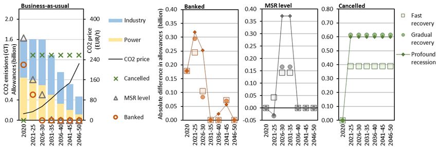
Figure 5 shows the outcome of different ratios for the business-as-usual and the three pandemic
scenarios by depicting the absolute level of cancelled allowances. As for the default ratio, cancelling
is the lowest under BAU, and highest under profound recession. Thus, changing the ratio does
not fundamentally changes the dynamics of the MSR in response to different COVID-19 scenarios.
Moreover, the ordering between ratios is the same for all four settings.
However, assumptions about the ratio fundamentally change the absolute level of cancelling.For
19Figure 5: CO2 emissions, prices, banked allowances, and the MSR
instance, cancelling is 21% higher for the +50% ratio and 26% lower with a –50% ratio. Additionally,
the absolute impact of different ratios is persistent across scenarios (around 0.15 to 0.42 billion more
cancelled allowances under fast recovery, 0.37 to 0.59 billion under gradual recovery, and 0.65 to
0.83 billion under profound recession) with the highest impact observed for –50%. Less pronounced
changes of the ratio (+10% and –10%) do not have a significant impact on the results of our analysis.
7 Conclusion
We determine the short-term (2020) and long-term (2021 to 2050) impacts of the COVID-19 pandemic
on the EU ETS including the MSR. We show detailed functioning of supply/demand of/for allowances,
banked allowances, movements of allowances into the MSR, MSR level, cancelling of allowances in the
MSR, and resulting EUA/CO2 prices. We further calculate the resulting direct (via the pandemic)
and indirect (via the EU ETS including the MSR) impact on the European power market. Looking
at the long-term impact of the pandemic in three different scenarios, namely fast recovery, gradual
recovery, and profound recession, we find that the MSR is an effective instrument to deal with an
exogenous shock such as the COVID-19 pandemic, as resulting EUA prices and also CO2 emission
levels stabilize fast. Interestingly, the MSR performs better—with regard to the climate change
context and intended high emission abatement—under more severe and longer lasting impacts of the
pandemic.
20Without the COVID-19 pandemic, 2.16 billion allowances in the MSR would be cancelled. Consid-
ering the impact of the pandemic, 0.28 billion additional allowances are cancelled if economic activity
(i.e., industrial CO2 emissions and electricity consumption) recovers by 2021 (fast recovery), whereas
CO2 emissions drop by 0.11 Gt in 2020; meaning that firms are not reacting much in response to the
cancelling mechanism. The excess from the 2020 drop in CO2 emission is carried until 2023, where
the cancelling mechanism starts. Gradual recovery (profound recession), where the pandemic impacts
economic activity until 2025 (2050), leads to additional cancelling of 0.4 (0.65) billion allowances and
thus a higher level of abatement. Also in these two scenarios, firms’ capabilities to react to the
cancelling mechanism are limited due to lower economic activity.
Looking at the 2020 impact of the pandemic on the European power market, the clean conventional
technologies, gas and bioenergy, are those that lose most in absolute terms. Coal generation even
increases. Thus, the pandemic has a negative short-term impact on the emission intensity of the
European power market. Emission intensity tends to increase also in the long-run, because clean
technologies (wind, solar, Gas-CCS) are those that suffer most from lower electricity demand. This
effect is particulary strong and persistent under a profound recession.
Although the MSR was initially designed to deal with short-term variability in economic activ-
ity (and related CO2 emissions), it is also highly effective in handling exogenously given long-term
emission reductions; at least given the specific European context (high amount of banked allowances,
MSR level from 2019 including 0.9 billion allowances from backloading, time lag to initial cancella-
tion). Based on our analysis, we conclude that no further adjustments are necessary in response to
the COVID-19 pandemic to avoid long-term negative impacts on the emissions level in the EU.
A recent study by [9]—with similar focus on the efficiency of the MSR but substantial differences
in the modelling setting (assumption of emission allowance demand shocks)—finds also that the MSR
passes the test introduced by the COVID-19 pandemic. By mitigating the negative demand shock,
the COVID-19 pandemic has a very limited effect on EUA prices. Contrary to our finding, they
find lower cancelling under more persistent compared to shorter and milder shock scenarios. The
possible explanation for such differences could lay in the sensitivity of the MSR. We find that small
adjustments fundamentally change the dynamics of the MSR. For example, neglecting the existence
of higher wind turbines from 2036-40 onward, will lead to the same cancelling volume under gradual
recovery and profound recession. Also the introduction of a Green Deal reflecting reform of the EU
ETS, will lead to cancelling in gradual recovery close to the profound recession volume. These findings
underline the fickleness of the EU ETS when accounting for the MSR.
In particular, the reinforced cancelling mechanism—movements into the MSR increases the MSR
level (and cancelling potential) on the on side and simultaneously increase the likelihood of cancelling
21by lowering the cancelling threshold (previous year’s auctioning allowances) on the other side—make
it difficult to obtain completely (against any changes) robust projections.
However, our conclusion does not undermine the importance of intended adjustment of the EU
ETS in accordance to the new carbon-neutrality goals of the EU (Green Deal). On the contrary, we
demonstrate that policy interventions and introduction of instruments like the MSR are prerequisites
to reach long-term carbon-neutrality in the EU. Whereas we do not find that an exogenous shock,
such as the COVID-19 pandemic, contributes to climate change mitigation by boosting a major and
long-lasting decrease in CO2 emissions, we also do not see such shocks as a major obstacle.
22References
[1] Koch, N., Fuss, S., Grosjean, G. & Edenhofer, O. Causes of the eu ets price drop: Recession,
CDM, renewable policies or a bit of everything?—New evidence. Energy Policy 73, 676 – 685
(2014). URL http://www.sciencedirect.com/science/article/pii/S0301421514003966.
[2] Ellerman, A. D., Marcantonini, C. & Zaklan, A. The European Union emissions trading system:
ten years and counting. Review of Environmental Economics and Policy 10, 89–107 (2016).
[3] European Commission. EU ETS handbook. DG Climate Action, 138 (2015).
[4] Richstein, J. C., Émile J.L. Chappin & de Vries, L. J. The market (in-)stability reserve for EU
carbon emission trading: Why it might fail and how to improve it. Utilities Policy 35, 1 – 18
(2015). URL http://www.sciencedirect.com/science/article/pii/S0957178715300059.
[5] Perino, G. New EU ETS Phase 4 rules temporarily puncture waterbed. Nature Climate Change
8, 262–264 (2018).
[6] Bertram, C. et al. Complementing carbon prices with technology policies to keep climate targets
within reach. Nature Climate Change 5, 235–239 (2015).
[7] Rosendahl, K. E. EU ETS and the waterbed effect. Nature Climate Change 9, 734–735 (2019).
[8] Rosendahl, K. E. EU ETS and the new green paradox. Working Paper Series 2-2019, Norwegian
University of Life Sciences, School of Economics and Business (2019). URL https://ideas.
repec.org/p/hhs/nlsseb/2019_002.html.
[9] Gerlagh, R., Roweno, J. & Heijmans, K. E. R. COVID-19 tests the Market Stability Reserve.
Environmental and Resource Economics 1–11 (2020).
[10] Zhang, Y.-J. & Wei, Y.-M. An overview of current research on EU ETS: Evidence from its
operating mechanism and economic effect. Applied Energy 87, 1804 – 1814 (2010). URL http:
//www.sciencedirect.com/science/article/pii/S030626190900556X.
[11] Venmans, F. A literature-based multi-criteria evaluation of the EU ETS. Renewable and Sus-
tainable Energy Reviews 16, 5493–5510 (2012).
[12] Bel, G. & Joseph, S. Emission abatement: Untangling the impacts of the EU ETS and the
economic crisis. Energy Economics 49, 531 – 539 (2015). URL http://www.sciencedirect.
com/science/article/pii/S0140988315001061.
23You can also read