Analyzing glacier retreat and mass balances using aerial and UAV photogrammetry in the Ötztal Alps, Austria
←
→
Page content transcription
If your browser does not render page correctly, please read the page content below
The Cryosphere, 15, 3699–3717, 2021
https://doi.org/10.5194/tc-15-3699-2021
© Author(s) 2021. This work is distributed under
the Creative Commons Attribution 4.0 License.

Analyzing glacier retreat and mass balances using aerial and
UAV photogrammetry in the Ötztal Alps, Austria
Joschka Geissler1,4 , Christoph Mayer2 , Juilson Jubanski1 , Ulrich Münzer3 , and Florian Siegert5
1 3D RealityMaps GmbH, Dingolfinger Str. 9, Munich, 81673, Germany
2 Bavarian Academy of Science, Geodesy and Glaciology, Alfons-Goppel Str. 11, Munich, 80539, Germany
3 Department of Earth and Environmental Sciences, Section Geology (remote sensing), Ludwig-Maximilians-Universität

München, Luisenstr. 37, 80333 Munich, Germany
4 Faculty of Environment and Natural Resources, Albert-Ludwigs-Universität Freiburg, Friedrichstr. 39,

79098 Freiburg, Germany
5 Faculty of Biology, GeoBio Center, Ludwig-Maximilians-Universität München, Richard-Wagner-Str. 10,

80333 Munich, Germany

Correspondence: Florian Siegert (siegert@bio.lmu.de)

Received: 10 September 2020 – Discussion started: 27 October 2020
Revised: 18 June 2021 – Accepted: 29 June 2021 – Published: 6 August 2021

Abstract. We use high-resolution aerial photogrammetry to         for a more comprehensive and detailed analysis of climate-
investigate glacier retreat in great spatial and temporal de-     change-induced glacier retreat and mass loss.
tail in the Ötztal Alps, a heavily glacierized area in Austria.
Long-term in situ glaciological observations are available for
this region as well as a multitemporal time series of digi-
tal aerial images with a spatial resolution of 0.2 m acquired     1   Introduction
over a period of 9 years. Digital surface models (DSMs) are
generated for the years 2009, 2015, and 2018. Using these,        The impacts of climate change are widespread and clearly
glacier retreat, extent, and surface elevation changes of all     visible in the Alps (Rogora et al., 2018) but particularly
23 glaciers in the region, including the Vernagtferner, are       evident in the dwindling glacier resources (Beniston et al.,
analyzed. Due to different acquisition dates of the large-        2018; Sommer et al., 2020; Zekollari et al., 2019). Over the
scale photogrammetric surveys and the glaciological data,         past 100 years, the temperature in the European Alps, here-
a correction is successfully applied using a designated un-       after referred to as the Alps, has increased almost twice as
manned aerial vehicle (UAV) survey across a major part of         fast compared to the global average, resulting in nearly 2 ◦ C
the Vernagtferner. The correction allows a comparison of the      higher mean air temperatures (Auer et al., 2007; Marty and
mass balances from geodetic and glaciological techniques –        Meister, 2012). By the end of this century, mean air temper-
both quantitatively and spatially. The results show a clear in-   atures are expected to rise further by several degrees Celsius
crease in glacier mass loss for all glaciers in the region, in-   (Gobiet et al., 2014; Hanzer et al., 2018). Due to this ongoing
cluding the Vernagtferner, over the last decade. Local devi-      climate evolution, alpine glaciers may lose half of their vol-
ations and processes, such as the influence of debris cover,      ume by 2050 compared to 2017 (Zekollari et al., 2019). The
crevasses, and ice dynamics on the mass balance of the Ver-       response of glaciers to climatic variations is related to the
nagtferner, are quantified. Since those local processes are not   glacier mass balance that can be measured, among others,
captured with the glaciological method, they underline the        directly, using the glaciological method, or indirectly, using
benefits of complementary geodetic surveying. The availabil-      the geodetic method. For the latter, the volume change of a
ity of high-resolution multi-temporal digital aerial imagery      glacier is determined by integrating the elevation change be-
for most of the glaciers in the Alps provides opportunities       tween two surveys across the entire glacier surface. Volume
                                                                  change is then converted to mass change by incorporating

Published by Copernicus Publications on behalf of the European Geosciences Union.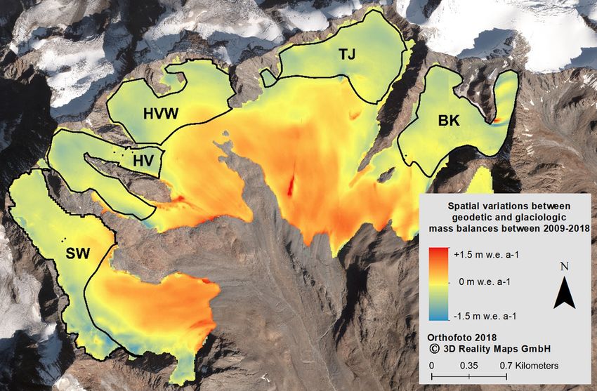
3700                                                                J. Geissler et al.: Analyzing glacier retreat and mass balances

a density assumption of the affected volume. For retrieving             each class (Pelto et al., 2019). However, those methods re-
geodetic mass balance data, different remote sensing meth-              quire extensive field measurements and computational effort.
ods exist, varying in the platform (e.g., satellite, airplane,          We present an easy applicable and transferrable approach, in-
UAV) and sensor (e.g., laser scanner, optic camera, radar)              corporating the equilibrium line altitude (ELA) of a glacier to
used. Their specific benefits and limitations are analyzed and          generate an altitude-related density assumption with a linear
discussed in different studies (Baltsavias et al., 2001; Bamber         transition around the ELA from firn to ice density. The re-
and Rivera, 2007; Kääb, 2005; Kargel et al., 2013; Pellikka             quired ELA can be retrieved from satellite imagery (Rabatel
and Rees, 2010).                                                        et al., 2005) or historic photographs (Vargo et al., 2017).
    Glaciological mass balances date back far into the last cen-           For the comparison of geodetic and glaciological data,
tury, and our knowledge of long-term glacier evolution is               extrapolating the mass balances to full mass balance years
based on these datasets (Mayer et al., 2013a; WGMS, 2020).              (30 September) (ii) is required, since survey dates usually
However, glaciological mass balances are limited to a few               differ. Such corrections can for instance be applied by using
glaciers only, due to the large effort involved in the field            a simple degree-day model (Belart et al., 2019) or field mea-
work. Existing historic aerial imagery can also provide valu-           surements (Fischer et al., 2011). These methods, however,
able information on long-term glacier evolution and, depend-            are either not suitable for retrospective corrections where no
ing on the imagery, allow a retrospective determination of              field data were collected or do not account for the spatially
geodetic glacier mass balances for a considerable number of             distributed, glacier-specific accumulation and ablation pat-
glaciers and thus greatly complement glaciological data (Be-            terns of each glacier (Huss et al., 2009). We present a work-
lart et al., 2019; Jaenicke et al., 2006; Magnússon et al., 2016;       flow for using an UAV survey with 5 cm spatial resolution, in
Mayer et al., 2017). Different studies demonstrate the poten-           combination with a simple degree-day model to correct dif-
tial of spatiotemporal change analysis of alpine glaciers using         ferences in survey dates between geodetic and glaciological
photogrammetric data (Fugazza et al., 2018; Gudmundsson                 data. This robust approach allows a more detailed analysis
and Bauder, 1999; Legat et al., 2016; Rossini et al., 2018) and         of the ice dynamics and the remaining systematic differences
comparing their results to glaciological mass balances (Balt-           between the geodetic and glaciological mass balances.
savias et al., 2001; Klug et al., 2018). Comparing geodetic                This study is focused on a study site within the Ötztal
and glaciological mass balances generally has the potential             Alps, Austria. Airborne photogrammetric datasets covering
to reveal systematic errors and regions of anomalous mass               23 glaciers are provided by the Austrian Bundesamt für Eich-
balance conditions (Fischer, 2011). However, when compar-               und Vermessungswesen (BEV) and 3D RealityMaps GmbH
ing these methods one needs to account for different error              for 2009, 2015, and 2018, thus covering a period of 9 years.
sources such as differences in survey dates, errors related             One of the surveyed glaciers is the Vernagtferner, a reference
to the density assumption, ice dynamics, internal and basal             glacier in the World Glacier Monitoring Service (WGMS)
melt, and other systematic or random error sources (Pellikka            system. Glaciological mass balances have been determined
and Rees, 2010; Zemp et al., 2013).                                     here using the glaciological method since 1965, while a se-
    Zemp et al. (2013) provide a framework to perform ho-               ries of historical maps back to 1889 demonstrates the long-
mogenization, error assessment, and calibration of the geode-           term glacier evolution over more than a century (Escher-
tic and glaciological datasets that is often used in the scien-         Vetter et al., 2009).
tific community (Andreassen et al., 2016; Klug et al., 2018).              Within this study, we describe the full photogrammetric
Building on this framework, considering the required addi-              workflow applied to our aerial imagery. After the coregistra-
tional data are available, we see further potential (i) regard-         tion of the resulting digital elevation models (DEMs), vol-
ing the involved density assumption as well as (ii) for extrap-         ume changes and general glacier retreat are analyzed for all
olating geodetic mass balances to full mass balance years.              23 glaciers. A more detailed analysis is conducted for the
These small improvements increase the detail of our geode-              Vernagtferner, where our altitude-related density assumption
tic mass balance and thus allow a more in-depth comparison              and the UAV-based correction of survey dates allow a spatial
of the geodetic and glaciological mass balances and will be             and quantitative comparison of the geodetic with the glacio-
presented within this study.                                            logical mass balances.
    Regarding volume-to-mass conversion (i), the simple den-
sity assumption provided by Huss (2013) is frequently used
to derive overall geodetic mass balances (Andreassen et al.,            2   Study area
2016; Belart et al., 2019). However, this assumption is only
valid for periods longer than 3 to 5 years, medium to high              The Ötztal Alps are located in the central-eastern Alps and
volume change, and stable mass balance gradients (Huss,                 represent one of Austria’s most extensive glacierized regions,
2013; Zemp et al., 2013). These strong limitations are often            covering a range in altitude between 1700 to 3768 m a.s.l.
overcome by using firn densification models (Reeh, 2008),               (meters above sea level) and more than 250 km2 (Fig. 1). It
existing field datasets (Huss et al., 2009), or pixel-based clas-       combines the upper regions of the drainage basins of Rofen-
sifications of snow, firn, and ice and assigning a density to           tal, Pitztal, and Kaunertal. The location in the inner part of

The Cryosphere, 15, 3699–3717, 2021                                                        https://doi.org/10.5194/tc-15-3699-2021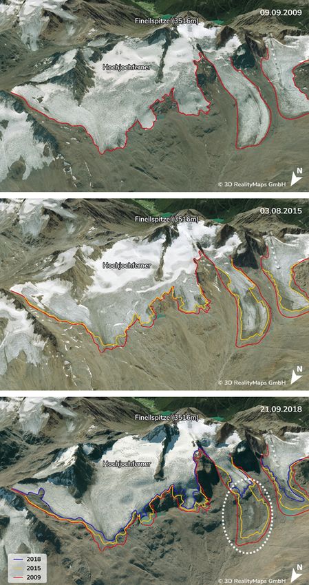
J. Geissler et al.: Analyzing glacier retreat and mass balances                                                             3701

the Alps leads to relatively low precipitation amounts (Fliri,    nation of density by using spring scales (about 4 %). There-
1975, pp. 186–197), which for example reach mean values of        fore water equivalent accuracy is about 6 % (Zemp et al.,
660 mm yr−1 at the Vent valley station in 1969–2006 (Aber-        2013). The typical number of stakes used for the annual mass
mann et al., 2009).                                               balance measurements at the Vernagtferner is about 35, while
   For some of the 23 glaciers within the study site, glacio-     4–5 accumulation measurements are collected at the end of
logical mass balance measurements exist. One of the longest       the glaciological year, 30 September.
series of measurements can be found at the Vernagtferner,            Glacier boundaries for delineating the spatial mass balance
where regular monitoring by the Bavarian Academy of Sci-          distribution are derived from aerial surveys repeated roughly
ences and Humanities (BAdW) began in 1965 (Escher-Vetter          every decade, updated in the ablation region by annual GNSS
et al., 2009). This glacier is characterized by several sub-      (Global Navigation Satellite System services) measurements
basins, which were connected to a single glacier tongue in        of the glacier tongue geometry. The spatial error of these
former times. In 2018, the glacier covered almost 7 km2           measurements is usually better than 1 m. The information
within an altitude range between 2860 and 3570 m a.s.l. The       from the stake readings, the depth soundings, the snow and
mass balance is determined by the glaciological method, us-       firn pits, and the location of the equilibrium line is combined
ing measurements at ablation stakes, using manual and geo-        to interpolate the spatial distribution of the glacier mass bal-
physical depth soundings, and retrieving information from         ance into a raster file. Due to the sparse information in the
snow and firn pits. The annual and winter mass balances are       accumulation region, it is necessary to manually correct the
determined independently of each other by measurements on         interpolation results in this region with the knowledge of the
the fixed dates of 1 May and 30 September, the dates of           long-term accumulation patterns, which are rather persistent.
the glaciological balance year (Cogley, 2010; Cogley et al.,      Errors introduced by uncertainties in the accumulation re-
2011). Besides, there is a long history of geodetic mapping at    gion, however, are relatively small, especially during the re-
the Vernagtferner dating back to 1889 (Mayer et al., 2013a).      cent decade where the accumulation area ratio (AAR) is usu-
                                                                  ally well below 30 %. While ablation varies between 0 and
                                                                  up to 4.5 m w.e. a−1 in the ablation area, accumulation only
3     Data acquisition                                            varies between 0 and about 0.3–0.4 m w.e. a−1 in the accu-
                                                                  mulation area. Within this study, we assumed the error of the
3.1    Photogrammetric data
                                                                  interpolated glaciological raster to be 0.1 m w.e. a−1 , which
In Austria, cadastral aerial surveys are conducted by the BEV     is in accordance with Zemp et al. (2013). It must be noted
with a nominal resolution of 0.2 m. We use a BEV survey           that this relatively large error within the accumulation area
from 2015 as a basis for our investigations. Besides, surveys     will only affect the final mass balance by less than 2 %.
performed by 3D RealityMaps in 2009 and 2018 with the                The ELA is derived by comparing oblique terrestrial pho-
same or higher ground resolution are investigated. Table 1        tographs of the transient snow line and firn extent with op-
shows the most relevant information on the conducted air          tical remote sensing information close to the field measure-
surveys.                                                          ments date. The derived ELA has a horizontal location accu-
   In addition to the airplane-based surveys, a smaller test      racy of about 10 m.
site was covered by an UAV flight to retrieve high-resolution
data at another acquisition date closer to the maximum of         4     Methods
ablation in 2018 (Table 1). The processed area covers 6 km2
containing most of the Vernagtferner, including all glacier       4.1     Photogrammetric workflow
tongues. The glacier was almost snow-free at the time of the
acquisition, which provides optimal processing conditions.        To determine geodetic glacier mass balances from aerial and
                                                                  UAV images, we used a workflow consisting of two main
3.2    Glaciological mass balance data                            modules: the data processing (Sect. 4.1.1) and the vertical
                                                                  change analysis (Sect. 4.1.2; Fig. 3). The main goal of the
Glaciological mass balance data are gathered as stake read-       data processing module was the reconstruction from raw
ings from ablation stakes for estimating the ice melt across      imagery data into 3D point clouds. Digital surface models
the glacier. Snow depth and last-season firn deposits are         (DSMs) and orthophotos were then derived from these point
determined from mechanical depth soundings with metal             clouds. Finally, DSM differences were computed. Within the
probes, which are then combined with density information          vertical change analysis module, geodetic glacier mass bal-
from snow and firn pits to calculate the water equivalent of      ances were computed from the DSM differences.
the remaining snow and firn cover. While stake readings only
require two length measurements per stake with an uncer-          4.1.1    Data processing
tainty of typically about 1 cm, more significant errors are in-
cluded in the direct accumulation measurements due to un-         The first step in data processing was the aerotriangulation,
certainties in the sample volume (about 5 %) and the determi-     which consists of the orientation of the aerial imagery to

https://doi.org/10.5194/tc-15-3699-2021                                                The Cryosphere, 15, 3699–3717, 2021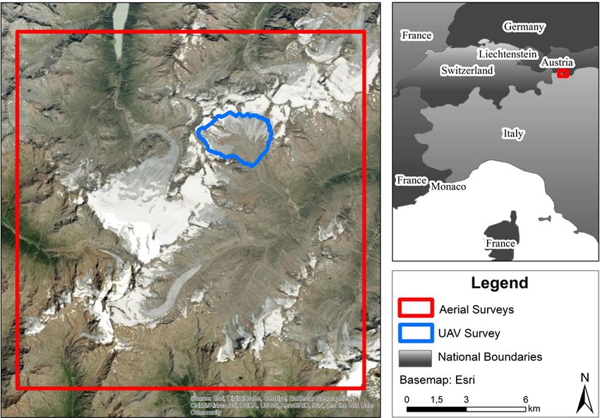
3702                                                               J. Geissler et al.: Analyzing glacier retreat and mass balances

Figure 1. Study site in the Ötztal Alps. Red shows the area covered by aerial surveys; blue shows the area of the Vernagtferner covered by
the UAV survey. Image source: ESRI (2020).

Table 1. Overview of the aerial data acquisitions.

         Date              Platform     Area     Overlap          Resolution    Images    Image type    Camera
         (dd.mm.yyyy)                  [km2 ]    (forward:side)        [cm]    [Count]
                                                 [%]
         09.09.2009        Airplane       257    80:40                   20        381    TIF RGB       UltraCam XP
                                                                                          8bit
         03.08.2015        Airplane       330    80:50                   20        572    TIF RGBI      UltraCam XP
                                                                                          16bit
         21.09.2018        Airplane       260    80:60                   20        428    TIF RGBI      UltraCam Eagle Mark 2
                                                                                          16bit
         21.08.2018        UAV              6    80:80                    5       1992    JPEG RGB      UMC-R10C
                                                                                          8bit

the real terrain. Modern photogrammetric survey systems de-            algorithm (Heipke, 2017; Hirschmüller, 2019) was used.
liver highly accurate positions using GNSS and orientation             This algorithm was implemented within the software SURE
(IMU, inertial measurement unit) information for each im-              (nFrames), which generates DSM and orthophotos from the
age, which were also included in the aerotriangulation for             point clouds. The horizontal shift of the derived orthopho-
the georeferencing. Finally, at least 20 tie points were man-          tos and DSMs was computed based on ground control points
ually identified for each image block to enhance the orienta-          from the BEV and lies between 10 and 20 cm depending on
tion accuracy. For the large-format imagery, the aerotriangu-          the acquisition year and thus within the ground resolution
lation was performed using the software Inpho (Match-AT)               of the images. Due to these excellent values, only a vertical
by Trimble. For the UAV imagery, the software Metashape                coregistration of the DSM differences was applied. There-
Professional from Agisoft was used.                                    fore, existing systematic height shifts between all DSMs
   The second stage of data processing was the generation              were derived using 50 stable points (e.g., solid rock) outside
of point clouds through three-dimensional reconstruction.              the glaciers. A total of 21 stable points were used for the UAV
For this purpose, the state-of-the-art semi-global-matching            survey. The 2015 DSM was chosen as the reference because

The Cryosphere, 15, 3699–3717, 2021                                                         https://doi.org/10.5194/tc-15-3699-2021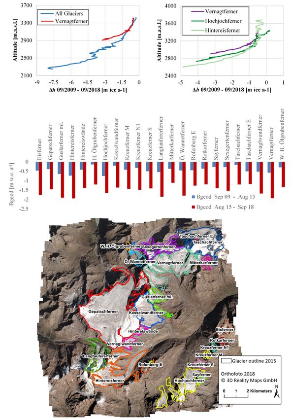
J. Geissler et al.: Analyzing glacier retreat and mass balances                                                                          3703

it was derived from the official Austrian cadastral survey and                dently according to the steps 1 to 4 in Zemp et al. (2013).
is referenced to the Austrian national survey system. Based                   Datasets were homogenized (Sects. 3.2 and 4.1.1), and an-
on this mean vertical shift over stable ground, all DSMs ex-                  nual glaciological mass balances were accumulated for the
cept for the reference DSM were adjusted in height rela-                      periods September 2009–September 2015, September 2015–
tive to the reference DSM of 2015. Subsequently, the DSM                      September 2018, and September 2009–September 2018,
differences September 2018–August 2015, August 2015–                          and mean annual mass balances of the respective periods
September 2009, September 2018–September 2009, and                            (Sects. 3.2 and 4.1.2) as well as systematic and random er-
September 2018–August 2018 were computed.                                     rors for all geodetic datasets (Sect. 4.3) were derived (Nuth
                                                                              and Kääb, 2011). Because one main objective of this paper
4.1.2    Vertical change analysis                                             was to analyze systematic differences between the two meth-
                                                                              ods, iterative adjustment and calibration of the data (step 5–6,
The goal of the vertical change analysis (Fig. 2, orange part)                Zemp et al., 2013) was not performed.
was to quantify elevation changes 1ht within our study area                      We developed a workflow to account for the remain-
from the DSM differences of different time periods t. By in-                  ing temporal differences between the photogrammetric and
tegrating 1ht over a specific area St , volume change 1V was                  glaciological mass balance data. Correction periods were de-
determined by the following equation, where r is the pixel                    fined between the survey date of the photogrammetric data
size (Fischer, 2011; Zemp et al., 2013):                                      and the end of the glaciological year (Table 2). An ad-
             Z St
                                                                              ditional photogrammetric DSM difference was derived for
1Vt = r 2 ×       1ht .                                   (1)                 1 month within the ablation period in 2018 (t = corr) using
                      0
                                                                              an UAV survey (Table 1). Therefore, a regression (sigmoid;
To derive overall geodetic glacier mass balances Bgeod,t , 1Vt
                                                                              see Fig. 3) was performed for deriving the altitude-dependent
was determined with St being the area at the beginning of
                                                                              surface elevation change 1hk,t=corr (Table 2) of the respec-
the respective period t (Fischer, 2011). St was digitized vi-
                                                                              tive period t = corr (Table 2). By multiplying 1ht=corr with
sually using orthophotos at a scale of 1 : 2000. For the fol-
                                                                              the altitude-related density assumption ft,d (e) (Eq. 3) the
lowing volume-to-mass conversion (Zemp et al., 2013), we
                                                                              mass balance Bgeod,e,t=corr for all elevation bins e and the
used the density assumption proposed by Huss (2013) (ρ =
                                                                              correction period t = corr (Table 2) was derived. Only those
850 kg m−3 ± 60 kg m−3 ) for all glaciers.
                                                                              altitude levels which were at least 40 % covered by the UAV
                 1V  ρ               St=begin + St=end                        survey were considered for the regression. The standard de-
Bgeod,t =        ×        with S =                         (2)
             S     ρwater                    2                                viation (SD) of the regression is 0.07 m ice (Fig. 3). Above
To allow a detailed analysis of the altitudinal dependencies                  3180 m a.s.l., thus, for the accumulation areas, the correction
of the glacier mass balances, the glacier area was divided                    function is not based on any data and is therefore error-prone.
into 10 m elevation bins e. For each bin, the geodetic mass                      To transfer this information to the correction periods (t =
balance Bgeod,e,t was derived with the same equations (see                    1 − 3, Table 2), we used temperature time series measured
Eqs. 1, 2 and Zemp et al., 2013).                                             at a climate station close to the Vernagtferner at 2640 m a.s.l.
   In contrast to most of the glaciers within our study area,                 Positive degree-day sums (PDDe,t ) [◦ C] were computed for
the ELA (Sect. 3.2) of the Vernagtferner is known and lies at                 all elevation bins e and time periods t (Table 2). To deter-
3217 m a.s.l. for the period 2009–2015, 3278 m a.s.l. for the                 mine the degree-day function (DDF) for all elevation bins,
period 2015–2018, and, averaged over the entire study pe-                     we assumed the vertical lapse rate of the air temperature to
riod, at 3237 m a.s.l. for 2009–2018. Thus, we were able to                   be −0.6 ◦ C per 100 m of altitude (Eq. 4). More information
use an altitude-related density function ρ = ft,d (e) for con-                on the DDF method can be found, for instance, in Braithwaite
verting surface changes to mass relative to the altitude of                   and Zhang (2000) and Hock (2003).
the ELA for the Vernagtferner (Fig. 2). This density func-
                                                                                           Bgeod,e,t=corr
tion ft,d (e) [kg m−3 ] represents the gradual change from ice                DDFe =                                                       (4)
density (900 kg m−3 ) in the ablation region to firn density                            PDDe,t=corr × dt=corr
(550 kg m−3 , Cogley et al., 2011) in the accumulation region                 The geodetic mass balance for the correction periods Be,t
with elevation e, by using a linear transition zone of ±50 m                  could then be determined for the time periods t of length dt
around the ELA of the respective period t:                                    and in all elevation bins e:
             (
                 550                       for e > ELA + 50 m
ft,d (e) =       725 − 3.5 × (e − ELAt )   for e between ELA ± 50 m   . (3)   Bgeod,e,t = DDFe × PDDe,t × dt .                             (5)
                 900                       for e < ELA − 50 m

                                                                              Subsequently, the geodetic mass balances of the full
4.2     Comparison with glaciological data                                    study periods Bgeod,e,09/2009–08/2015 , Bgeod,e,08/2015–09/2018 ,
                                                                              and Bgeod,e,09/2009–09/2018 were corrected according to Ta-
To allow a comparison of the geodetic and glaciologi-                         ble 2 and recalculated to an annual basis. In this study, we
cal mass balances, both datasets were reanalyzed indepen-                     refer to these temporally corrected geodetic mass balances

https://doi.org/10.5194/tc-15-3699-2021                                                             The Cryosphere, 15, 3699–3717, 2021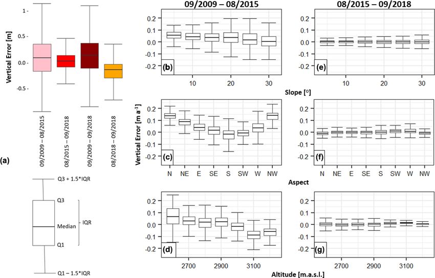
3704                                                                        J. Geissler et al.: Analyzing glacier retreat and mass balances

Figure 2. Full workflow. Blue shows the data processing steps from raw images to DSM differences; orange shows the vertical change
analysis performed to determine altitudinal and overall mass balances.

Table 2. Correction parameters (left) of all correction periods t and the applied corrections to all geodetic mass balances (right).

    t          Correction periods         dt   PDDe=2870 m a.s.l.,t     Applied corrections
                                      [days]                [◦ C]
    1      09.09.2009    30.09.2009       21                82.45       Bgeod,e,09−15 = Bgeod,e,09/2009–08/2015 − Bgeod,e,t=1 + Bgeod,e,t=2
    2      03.08.2015    30.09.2015       59               280.76       Bgeod,e,15−18 = Bgeod,e,08/2015–09/2018 − Bgeod,e,t=2 + Bgeod,e,t=3
    3      21.09.2018    30.09.2018        9                46.58       Bgeod,e,09−18 = Bgeod,e,09/2009–09/2018 − Bgeod,e,t=1 + Bgeod,e,t=3
    corr   21.08.2018    21.09.2018       31               176.81

as annual geodetic mass balances (unit: m w.e. a−1 ) and pro-                   method). Therefore, we digitized the respective areas on the
vide the information on the period with full years (e.g., 2009–                 Vernagtferner by using the geodetically derived orthophotos
2018). Uncorrected geodetic mass balances are referred to                       of 2009 and 2018 and computed the mean annual variation
by year and their respective month (e.g., September 2009–                       (difference between the annual geodetic and the glaciolog-
September 2018).                                                                ical mass balances) by using the variation raster (Eq. 7) as
   The overall geodetic mass balances Bgeod,t of the Vernagt-                   well as Eqs. (1) and (2). By comparing this mean variation
ferner were then derived from the mass balances of the single                   with the mean variation of areas within the same elevation
elevation bins e and their respective area Se,t (Zemp et al.,                   bin, we estimated the magnitude of error introduced by ne-
2013):                                                                          glecting those areas within glaciological mass balances.
           PE
                Bgeod,e,t × Se,t                                                4.3   Vertical accuracy assessment
Bgeod,t = e=1                    .                           (6)
                   St
                                                                                To assess the error distribution within the study area after the
Finally, accumulated glaciologically derived rasters Bglac,t                    coregistration, temporally uncorrected geodetic DSM differ-
(Sect. 3.2) were subtracted from the adjusted geodetic mass                     ences were analyzed following the methodology presented
balances Bgeod,t . The resulting variation rasters Vart show the                by Nuth and Kääb (2011). Therefore, 1.5 km2 of ice-free,
spatial deviations between the two methods, where negative                      stable terrain representing a wide range of topography was
values occur for areas where Bglac,t > Bgeod,t and positive                     digitized manually. The mean shift and the SD within those
values occur for the opposite relation.                                         areas were calculated, and their relation to topography was
Vart = Bgeod,t − Bglac,t                                              (7)       investigated. To estimate the error when averaging over ex-
                                                                                tended areas, we followed Rolstad et al. (2009) by assessing
Using this variation raster, we analyzed spatial deviations                     the spatial covariance of the elevation differences using semi-
between both methods that occur due to differences in the                       variograms. Thus, we derived range values from the semivar-
individual methods and related errors (e.g., neither includ-                    iograms of all periods and converted those to the confidence
ing the supra-glacial debris cover or crevassed areas for sur-                  interval of the respective DSM difference. For more detailed
face ablation nor dynamic processes within the glaciological                    information on this method, see Rolstad et al. (2009). For

The Cryosphere, 15, 3699–3717, 2021                                                                 https://doi.org/10.5194/tc-15-3699-2021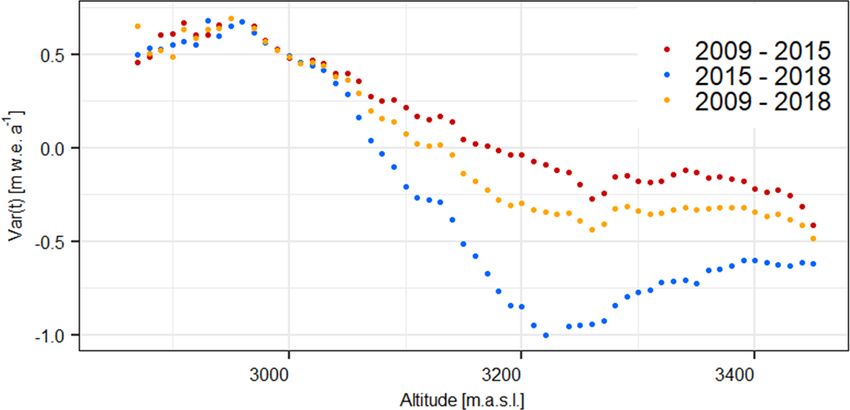
J. Geissler et al.: Analyzing glacier retreat and mass balances 3705
Figure 3. Surface changes in 10 m altitude bins for the correction period (21 August 2018 to 21 September 2018, red dots); the regression
curve (yellow) represents height changes related to the altitude; SD of the regression is 0.07 m ice.
the application of the method, we assumed that elevation dif- 5.1.2 Vertical accuracy assessment
ferences are constant in space, that they do not contain any
large-scale trends, and that there is no significant variation of The accuracy assessment (Sect. 4.3) allows an estimation of
the variance in space. potential error related to the DSM differences and derived
Basic error propagation was implemented (Nuth and Kääb, products. In general, the mean vertical error of the DSM
2011; Zemp et al., 2013) to determine the compound error differences ranges from −0.16 to 0.10 m, SD does not ex-
of DSM differences, density conversion (7 %, Sect. 4.1.2, ceed 0.42 m (Fig. 6a), and errors are generally smaller for
Huss, 2013), the correction function of the acquisition dates the period August 2015–September 2018. As expected, SD
(SD = 0.07 m ice a−1 , Sect. 4.2), and the error associated increases with the slope for both periods (Fig. 6b, e). An ap-
with the glaciological interpolation raster (Sect. 3.2) for all parent increase in the SD can also be found in lower altitudes
presented results. The error within this study is indicated by (< 2600 m a.s.l., (Fig. 6d, g), most likely due to the increas-
the 95 % confidence interval. ing influence of vegetation. A relation between aspect and
the vertical error was found for the DSM difference Septem-
ber 2009–August 2015 (Fig. 6c), which can be attributed to
5 Results a horizontal shift of the DSM 2009 (Sect. 4.1.1) (Nuth and
Kääb, 2011).
5.1 Vertical change analysis
5.1.1 Visual assessment 5.1.3 Mass balances
Using the derived glacier outlines, orthophotos, and DSM Volumetric changes 1Vt,e and height changes 1h(t, e) for
differences, the first results are obtained by a visual inter- every elevation bin e were derived for all periods t and all
pretation for the entire study area. In general, glaciers have glaciers, before and (for the Vernagtferner only) after the cor-
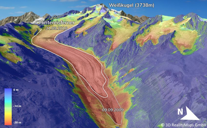
thinned and reduced in size. For instance, surface height rection of acquisition dates (Eqs. 1–2, Fig. 7).
changed at the glacier tongue of the Hintereisferner by up Before and after the temporal correction, the annual height
to −20.4 ± 0.4 m during the 9 years from September 2009 changes per elevation bin show a characteristic shape, with
to September 2018 (Fig. 4). With increasing altitude, the height changes being the most negative at the glacier tongues.
loss of height on the glacier approaches zero. Surface eleva- The period between 2009 and 2015 generally shows less neg-
tion changes around the glacier tongue of the Hintereisferner ative values than the period 2015 and 2018 in all altitudes for
can be attributed, among others, to local debris movements all glaciers (Fig. 7, bottom left) and the Vernagtferner (Fig. 7,
and an existing dead-ice body (Fig. 4). Analyzing the or- top left). Although, after the temporal correction the differ-
thophotos of the three surveys reveals that the eastern part of ence in height change between the two periods is consider-
the Hochjochferner lost a considerable area along its lower ably smaller.
glacier margin. In particular, its main tongue shortened by Compared to the height changes, the most negative vol-
826.4 ± 0.2 m between 2009 and 2018 (Fig. 5, white dotted ume change occurs in higher elevations since it is linked to
circle). Further visualization of the DSM differences can be the area–height distribution of a glacier. After correcting for
assessed at https://og.realitymaps.de/AlpSense/ (last access: the acquisition dates, based on a regression curve (Gaussian
22 July 2021). fit) for the values of the Vernagtferner, between 2009 and
2015, the most negative volume change of −0.21 ± 0.01 mil-
lion cubic meters per year occurred at an altitude of 3009–
https://doi.org/10.5194/tc-15-3699-2021 The Cryosphere, 15, 3699–3717, 2021
3706                                                                J. Geissler et al.: Analyzing glacier retreat and mass balances

Figure 4. Three-dimensional representation of the color-coded height differences in meter (m) between the DSMs of September 2009
and September 2018 for Hintereisferner (white outline). Surface elevation loss appears in red; constant elevation appears blue. Ice loss is
especially high at altitudes below 2500 m. The underlying orthophoto was derived from the 2018 aerial survey. Height loss in the southeast
of the glacier tongue can likely be attributed to an existing dead-ice body.

3019 m a.s.l. Between 2015 and 2018, the most negative vol-             glected within the glaciological method. Debris cover above
ume change further decreased to −0.29 ± 0.02 million cubic              a certain thickness protects the glacier against incoming heat
meters per year at an increased altitude of 3089–3099 m a.s.l.          fluxes (Östrem, 1959) and therefore reduces the ablation.
(Fig. 7, top right). The same trend was found for all glaciers          With our variation raster, we were able to quantify the ef-
within the study area, although no correction was applied to            fect of neglecting debris-covered areas within the glaciolog-
those values (Fig. 7, bottom right).                                    ical interpolation: for 2018, a total area of 91 350 m2 (1.5 %
                                                                        of the total area of the Vernagtferner) at a mean altitude
5.2    Comparison with glaciological measurements                       of 3040 m a.s.l. was classified as debris cover. The varia-
                                                                        tion between the geodetic and glaciological method for those
The geodetic and glaciological mass balances of the Vernagt-            debris-covered areas is 0.56 ± 0.3 m w.e. a−1 and thus more
ferner were further compared to detect discrepancies in spa-            positive than the mean variation at the respective altitude
tial distribution or magnitude between both methods. As al-             0.38 ± 0.27 m w.e. a−1 (period 2009–2018; see Fig. 9). Con-
ready noted, the overall mass balance for the Vernagtferner             sidering the difference of those values, the overall glaciolog-
is more negative in the period 2015–2018 than in the period             ical mass balance of 2009–2018 would be 0.17 m w.e. a−1
2009–2015. This can be seen in both the glaciological and the           (2 %) less negative if debris-covered areas were considered
geodetic mass balances (Fig. 8). The uncorrected geodetic               in the interpolation.
mass balance (blue) does not equal the corresponding glacio-               Further analysis of the variation raster (Fig. 10) empha-
logical mass balance (orange). After the correction of acqui-           sizes that geodetic and glaciological mass balances do not
sition dates (red), the annual geodetic mass balance has ap-            only differ due to debris cover or other local effects. More
proached the glaciological data. However, the corrected data            precisely, it is evident that the deviations depend on the al-
are still more negative for 2015–2018 and 2009–2018. For                titude. Thus, in the lower parts of the glacier, the geodetic
the period 2009–2015, corrected geodetic and glaciological              mass balance is less negative than the glaciological mass bal-
mass balances match.                                                    ance. For higher altitudes, the geodetic mass balance is more
    The spatial differences between both methods were further           negative than the glaciologically derived one. This pattern is
investigated using the variation raster described in Sect. 4.2.         usually attributed to the ice dynamic component of elevation
It is noticeable that the variation raster is more positive (thus       change contained in the geodetic differences (submergence
Bglac,t < Bgeod,t ; see Eq. 7) in debris-covered areas compared         and emergence of ice and firn). Additionally, Fig. 9 clearly
to its surrounding cells (red in Fig. 10). Since no ablation            shows that, comparing the different observation periods, the
stakes are located in supra-glacial debris at the Vernagtferner         bias between both methods becomes larger within the accu-
and glaciological mass balances are interpolated from sur-              mulation areas.
rounding information on clean ice, the effect of debris is ne-

The Cryosphere, 15, 3699–3717, 2021                                                          https://doi.org/10.5194/tc-15-3699-2021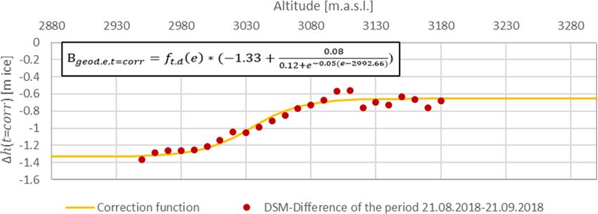
J. Geissler et al.: Analyzing glacier retreat and mass balances                                                                        3707

Figure 5. Three-dimensional visualization of the length change for the Hochjochferner in 2009 (top), 2015 (middle), and 2018 (bottom);
lines indicate glacier extent for the respective years. The second glacier tongue from the right (white dotted circle) lost 826 m in 9 years.

https://doi.org/10.5194/tc-15-3699-2021                                                         The Cryosphere, 15, 3699–3717, 2021
3708                                                                J. Geissler et al.: Analyzing glacier retreat and mass balances

Figure 6. Overall vertical error of the DSM differences (a); annual vertical error for the periods September 2009–August 2015 (b–d) and
August 2015–September 2018 (e–g) in relation to slope (b, e), aspect (c, f), and altitude (d, g).

Figure 7. Annual height changes 1h(t) per altitude for the Vernagtferner (a) and all glaciers (c); annual volume changes for the Vernagtferner
(b) and all glaciers (d); dotted lines represent the surface or volume changes after the correction of the acquisition dates.

  Assuming all variations between geodetic and glaciologi-               itive value being 0.7 ± 0.25 m w.e. a−1 . Submergence occurs
cally derived mass balances (Fig. 9) are caused by dynamic               at altitudes higher than 3150 m a.s.l. and results in a mean of
processes, the magnitude of emergence and submergence is                 −0.31 ± 0.25 m w.e. a−1 , with the most negative value being
computed using the variation raster and Eqs. (1) and (2). Be-            −0.48 ± 0.25 m w.e. a−1 (Fig. 10 and Table 3). For a glacier
tween 2009 and 2018, the mean emergence (between 2900                    in balance, the change between submergence and emergence
and 3050 m a.s.l.) is 0.55 ± 0.25 m w.e. a−1 , with a most pos-          regions occurs close to the equilibrium line. However, the

The Cryosphere, 15, 3699–3717, 2021                                                            https://doi.org/10.5194/tc-15-3699-2021
J. Geissler et al.: Analyzing glacier retreat and mass balances                                                                           3709

Figure 8. Comparison between geodetic mass balances (blue) and glaciological mass balances (orange) for the investigation periods. Red
bars visualize corrected geodetic data.

Figure 9. Methodical variations between annual geodetic (corrected) and glaciological mass balances, depending on the altitude [m w.e. a−1 ]
for all periods t; positive values are present where Bglac,t < Bgeod,t , and negative values are present for the opposite relation; see Eq. (7).

mean ELA of the Vernagtferner lies at 3237 m a.s.l. for the               ance is partly due to the temporal correction that was not
period 2009–2018 and thus roughly 150 m higher than the                   carried out. Thus, the mass balances do not refer to the
switch between apparent emergence and submergence.                        glaciological year and cannot be compared with glaciolog-
   When comparing the five different accumulation basins                  ical data. If a time correction is assumed to have a sim-
of the Vernagtferner, the derived submergence is more                     ilar influence on the mass balances of other glaciers as
negative for higher basins, with the largest offsets for                  it had for the Vernagtferner (−34 % for September 2009–
the remaining true accumulation regions Hochvernagt and                   August 2015, +20 % for August 2015–September 2018, and
Taschachhochjoch (Fig. 10 and Table 3).                                   +1.2 % for September 2009–September 2018, Fig. 8), the
                                                                          annual mass balances of all glaciers can be estimated. Ac-
5.3   Other glaciers within the study site                                cordingly, the annual glacier mass balance of all glaciers
                                                                          within the study area would be −0.61 ± 0.07 m w.e. a−1
The major advantage of geodetic mass balances compared to                 (2009–2015), −1.25 ± 0.14 m w.e. a−1 (2015–2018), and
glaciological mass balances is that large areas can be investi-           −0.83 ± 0.1 m w.e. a−1 (2009–2018). Based on this assump-
gated in great spatial detail. To highlight this benefit, we in-          tion, annual geodetic mass balances would have doubled be-
vestigated the geodetic mass balance of all glaciers within the           tween the two periods 2009–2015 and 2015–2018, and the
study area (Sect. 4.1.2). The temporally uncorrected geode-               annual geodetic mass balance of the Vernagtferner for the
tic mass balance of all glaciers is −0.46 ± 0.06 m w.e. a−1               same periods is 25 %, 21 %, and 22 % more negative than the
between September 2009 and August 2015, while it                          mean of all glaciers (Fig. 8).
quadruples to −1.59 ± 0.21 m w.e. a−1 between August 2015                    The remaining error due to the horizontal shift of the 2009
and September 2018. For the aggregated period (Septem-                    DSM (Sect. 5.1.2) is negligible for these general consider-
ber 2009–September 2018), the uncorrected geodetic mass                   ations but must be taken into account when working with
balance of all glaciers is −0.84 ± 0.11 m w.e. a−1 . It must              individual mass balances (Table 4, Fig. 11).
be noted that the quadrupling of the geodetic mass bal-

https://doi.org/10.5194/tc-15-3699-2021                                                           The Cryosphere, 15, 3699–3717, 2021
3710 J. Geissler et al.: Analyzing glacier retreat and mass balances
Figure 10. Variation raster 2009–2018: spatial variations of the annual geodetic (corrected) and glaciological mass balance data; blue areas
with negative variations represent areas where Bgeod,t < Bglac,t . In red areas, the opposite relation is present (see Eq. 7). For regions that
appear yellow, both methods present similar mass balances; black outlines represent the different accumulation areas of the Vernagtferner.
Table 3. Mean values of the variation raster 2009–2018 (Fig. 10) for the accumulation areas in m w.e. a−1 , interpreted as submergence; the
associated error is ±0.25 m w.e a−1 for all submergence values.
Accumulation area Mean submergence between Area > 3150 m a.s.l.
2009 and 2018 [m w.e. a−1 ] [km2 ]
SW Schwarzwand −0.26 0.69
HV Hochvernagt −0.38 0.44
HVW Hochvernagtwand −0.30 0.54
TJ Taschachhochjoch −0.41 0.56
BK Brochkogel −0.28 0.62
VN Vernagtferner (total) −0.32 2.85
6 Discussion We further evaluated the vertical surface height changes as
a function of elevation (Fig. 7). Even though they cannot be
This study investigated multitemporal changes in surface directly compared to glaciologically derived vertical balance
heights of selected glaciers in the Ötztal Alps with high spa- profiles, they illustrate the relation of height losses to alti-
tial resolution. We derived geodetic mass balances for 23 tude (Kaser et al., 2003; Pellikka and Rees, 2010). We found
glaciers within our study area and found that glacier mass that the elevation changes of all glaciers within our study
loss accelerated within the last decade. At the same time, the site (i) are on average less negative compared to the Vernagt-
absolute surface height changes showed a maximum at low ferner, (ii) are correlated to the altitude of the glacier tongue,
altitudes for all glaciers (Fig. 7). Peak volume loss occurs and (iii) increased between September 2009–August 2015
at higher altitudes, compared to the altitude where maximum and August 2015–September 2018 (Fig. 11). Besides glacier
surface height losses occur since the volume is directly linked analysis, surface elevation changes caused by other processes
to the area–height distribution of a glacier. These findings (e.g., dead-ice bodies, debris movement) can be identified
correspond to general observations (i) for the Vernagtferner using high-resolution photogrammetric data. For instance,
(BAdW, 2019; Escher-Vetter, 2015) and (ii) for most of the on the north-facing side of the valley, below the glacier
glaciers in the Alps (Davaze et al., 2020; M. Fischer et al., tongue of Hintereisferner, existing surface elevation changes
2015; A. Fischer et al., 2015; Huss, 2012). (Fig. 4), which can mostly be attributed to an existing dead-
ice body, were analyzed: over an area of 27×104 m2 , volume
The Cryosphere, 15, 3699–3717, 2021 https://doi.org/10.5194/tc-15-3699-2021Table 4. Surface changes [m] and geodetic mass balances [m w.e. a−1 ] of all glaciers within the study area. Geodetic mass balances were derived by using a fixed density factor
(Sect. 4.1.2 and Fig. 2); values are temporally uncorrected and thus do not match the glaciological year; glaciers marked with (*) must be considered with additional caution for
the periods September 2009–August 2015 and September 2009–September 2018 due to their orientation. Related errors are higher than the error estimates presented in this paper
(Sect. 5.1.2).
Name 1hk 1hk 1hk Bgeod Bgeod Bgeod Area 2009 Area 2015 Area 2018
09/2009–08/2015 08/2015–09/2018 09/2009–09/2018 09/2009–08/2015 08/2015–09/2018 09/2009–09/2018 [km2 ] [km2 ] [km2 ]
https://doi.org/10.5194/tc-15-3699-2021
[m] [m] [m] [m w.e. a−1 ] [m w.e. a−1 ] [m w.e. a−1 ]
Eisferner −3.29 −6.20 −9.48 −0.47 −1.76 −0.90 0.84 0.77 0.63
Gepatschferner −2.72 −5.15 −7.87 −0.39 −1.46 −0.74 18.95 18.78 18.59
Guslarferner mi. −4.54 −6.71 −11.24 −0.64 −1.90 −1.06 1.56 1.42 1.27
Hintereisferner −5.18 −6.85 −12.03 −0.73 −1.94 −1.14 7.13 6.44 6.10
Hintereiswände −2.98 −4.88 −7.86 −0.42 −1.38 −0.74 0.41 0.41 0.34
H. Ölgrubenferner −1.00 −4.23 −5.23 −0.14 −1.20 −0.49 0.06 0.06 0.05
Hochjochferner −5.26 −5.81 −11.08 −0.75 −1.65 −1.05 4.90 4.34 3.84
Kesselwandferner −1.44 −4.81 −6.25 −0.20 −1.36 −0.59 3.70 3.60 3.56
J. Geissler et al.: Analyzing glacier retreat and mass balances
Kreuzferner M (*) −2.97 −5.05 −8.02 −0.42 −1.43 −0.76 0.34 0.33 0.18
Kreuzferner N1 (*) −2.25 −5.23 −7.48 −0.32 −1.48 −0.71 0.27 0.25 0.21
Kreuzferner S (*) −3.53 −4.97 −8.50 −0.50 −1.41 −0.80 0.56 0.53 0.46
Langtaufererferner −3.84 −6.52 −10.36 −0.54 −1.85 −0.98 3.07 3.04 2.89
Mitterkarferner −2.61 −3.93 −6.54 −0.37 −1.11 −0.62 0.54 0.54 0.52
Ö. Wannetferner −3.25 −6.33 −9.58 −0.46 −1.79 −0.91 0.58 0.58 0.42
Rofenberg E (*) −3.15 −4.46 −7.62 −0.45 −1.26 −0.72 0.09 0.09 0.07
Rotkarferner (*) −2.55 −4.20 −6.75 −0.36 −1.19 −0.64 0.22 0.22 0.11
Sayferner (*) −1.95 −4.91 −6.86 −0.28 −1.39 −0.65 0.27 0.27 0.25
Sexegertenferner −1.96 −5.43 −7.39 −0.28 −1.54 −0.70 2.98 2.91 2.46
Taschachferner −1.14 −4.24 −5.38 −0.16 −1.20 −0.51 5.82 5.78 5.30
Taschachferner E. −3.57 −4.15 −7.72 −0.51 −1.18 −0.73 0.05 0.05 0.05
Vernaglwandferner −3.72 −5.94 −9.66 −0.53 −1.68 −0.91 0.75 0.70 0.58
Vernagtferner −4.05 −6.80 −10.85 −0.57 −1.93 −1.03 7.33 7.02 6.10
W.H. Ölgrubenferner −2.07 −4.72 −6.79 −0.29 −1.34 −0.64 0.14 0.14 0.13
The Cryosphere, 15, 3699–3717, 2021
37113712 J. Geissler et al.: Analyzing glacier retreat and mass balances Figure 11. Annual height changes per altitude between September 2009 and September 2018 for the Vernagtferner compared to (i) all glaciers within the study area (top left) and (ii) the Hochjochferner and Hintereisferner (top right); comparison of temporally uncorrected geodetic mass balances (Bgeod) of all glaciers within the study area for the two investigation periods (middle); glacier outlines of 2015 are shown on orthophoto 2018 (bottom). The Cryosphere, 15, 3699–3717, 2021 https://doi.org/10.5194/tc-15-3699-2021
J. Geissler et al.: Analyzing glacier retreat and mass balances                                                             3713

loss was quantified to be (1.3 ± 0.22)×106 m3 for the period         Derived geodetic mass balances (Table 4) are in
2009–2018.                                                        accordance with the literature. For instance, the de-
   The error assessment revealed the general high precision       rived geodetic mass balance of the Hintereisferner
of photogrammetric data with the SD of the vertical error not     (−1.14 ± 0.02 m w.e. a−1 , Table 4) for the period Septem-
exceeding 0.42 m for all DSM differences (Fig. 6). The varia-     ber 2009–September 2018 differs by only 8 % compared
tion of the vertical error is normally distributed and semivar-   to the glaciological mass balance of the same period
iograms determined to assess the error for averaged values        (−1.24 m w.e. a−1 (WGMS, 2020)), measured by the In-
show a sill for all periods (further information on the method    stitute of Atmospheric and Cryospheric Sciences of the
can be found in Rolstad et al., 2009). However, a relation        University of Innsbruck. However, since geodetic surveys
was found for the vertical error regarding the aspect for the     are not always possible at the end of the glaciological
period September 2009–August 2015 and September 2009–             year, there are large deviations (especially for the shorter
September 2018, which is presumably based on a horizon-           periods September 2009–August 2015 and August 2015–
tal shift of the DSM 2009 (Sect. 4.1.1). Thus, assumptions        September 2018) from the glaciological periods, and thus a
made hereupon (Sect. 4.3) are potentially less valid, mean-       direct comparison with glaciological mass balances is not
ing that the relation to the aspect can cause larger error bars   possible. As a result, the mass balances shown in Table 4 are
than we suggest. Especially for glaciers with homogeneous         influenced by the temporal offset, which causes parts of the
orientation to the north or northwest, presented values must      observed increase in mass balance magnitude. This must be
be considered with caution. However, only a few glaciers are      considered for any further use.
affected by this and are highlighted accordingly in this pa-         We developed a methodology to account for this tem-
per. By applying a full coregistration, following Nuth and        poral offset thus to adjust geodetic mass balances to the
Kääb (2011), this rotational error could have been addressed.     end of the glaciological year (30 September). An additional
   We used the density assumption of Huss (2013) to convert       UAV survey was conducted, which allowed assessing vertical
height changes to water equivalent for all glaciers except for    height changes during 1 month of the ablation period in 2018
the Vernagtferner, which is repeatedly used for volume-to-        (Fig. 3). Therefore, a regression function (sigmoid) was de-
mass conversions in other studies (Andreassen et al., 2016;       termined to estimate surface changes relative to the elevation.
Belart et al., 2019). All DSM differences fulfill the prereq-     We incorporated meteorological data from a nearby climate
uisites for this density assumption (Huss, 2013). However,        station by using a simple degree-day model for all relevant
the DSM difference for August 2015–September 2018, be-            periods and elevation bins. Our regression function includes
ing a rather short period of only 3 years, just meets those       uncertainty for the accumulation areas since the UAV survey
requirements. Thus, the density assumption and the de-            did not cover the entire glacier area. However, we showed
rived geodetic mass balances for this period must be con-         that the presented workflow provides good results as cor-
sidered with caution. For the Vernagtferner, we applied an        rected annual geodetic mass balances agree well with glacio-
altitude-related density function based on the known ELA.         logical mass balances (Fig. 8). Those results suggest that
Since the density of the glacier volume lost is related to the    our method is suited for retrospective corrections of geode-
ELA, our approach is more suitable for shorter time peri-         tic mass balances and can improve comparisons of geode-
ods where the influence of annual meteorological conditions       tic with glaciological mass balances. However, the method
is increased, compared to the static density assumption pro-      will perform best if the AAR and area–height distribution
vided by Huss (2013). For the Vernagtferner, ELA increased        remain similar between the period to be corrected and the
61 m between our two study periods 2009–2015 and 2015–            period of the determined correction function. Thus, the ret-
2018. This relatively small change in elevation changed the       rospective correction is limited to a few years only. The pre-
AAR of this glacier by about 15 % and thus has an influ-          sented method complements other existing correction meth-
ence on the density of the volume lost during those periods       ods that rely, for instance, on field data, available for only a
that should not be neglected. The presented density func-         few glaciers, or DDF models that do not have spatially ex-
tion accounts for such changes of the AAR and thus al-            plicit output (Belart et al., 2019; Fischer, 2011). It must be
lows a more detailed spatial comparison of the geodetic and       noted that our method was only tested on the Vernagtferner
glaciological mass balances. Since the ELA can be estimated       for a limited number of observation periods, and thus further
from satellite imagery (Rabatel et al., 2005), our method is      testing is required to assess its robustness and transferability
transferable to other glaciers. We recommend, however, ad-        to other glaciers and periods. Therefore, individual correc-
justing the firn density values to the corresponding region.      tion functions must be determined for each glacier individ-
The presented altitude-related density function is easily ap-     ually, as these are directly related to glacier-specific slope
plicable and needs low computational effort and therefore         gradients, orientation, the height of the glacier tongue, and
greatly complements other existing density conversion fac-        area–height distributions (Fig. 11). To determine such indi-
tors, which account for, e.g., firn compaction processes and      vidual correction functions, temperature information (for the
rely on classification methods or modeling (Pelto et al., 2019;   correction period as well as all periods to which the correc-
Reeh, 2008).                                                      tion is applied) and an additional geodetic survey is needed

https://doi.org/10.5194/tc-15-3699-2021                                                The Cryosphere, 15, 3699–3717, 2021
3714                                                                 J. Geissler et al.: Analyzing glacier retreat and mass balances

to estimate the surface elevation changes during the correc-             ELA for the period 2015–2018. While the ELA increased be-
tion period. The length of the correction period was 1 month             tween the two periods (2009–2015 vs. 2015–2018) by 61 m,
within this study; however, we do not expect poorer results              the change from submergence to emergence decreased by
if varying this period by 1–2 weeks. The required geodetic               about 130 m. The reasons for this development are unknown
survey is neither limited to a platform nor to a sensor. Thus,           but might indicate a further deviation from balanced con-
all geodetic survey configurations that allow the determina-             ditions during recent years. The derived submergence must
tion of geodetic glacier mass balances from DSM differences              be considered with high caution since it is neither validated
are suited for deriving the presented correction function. We            with field measurements nor model results. Presented sub-
used a dedicated photogrammetry-based UAV survey, flexi-                 mergence values are also based on (i) our applied correction
ble and low cost, that enabled a correction with high spatial            with sparse data for the accumulation region, (ii) the inter-
resolution.                                                              polation of a few glaciological stake readings, and (iii) our
   Comparing the corrected geodetic with interpolated                    assumption that internal and basal processes are negligible.
glaciological mass balance rasters revealed local deviations             Those values (Table 3) are thus error-prone and should only
(Fig. 10). They mainly occur in crevassed and debris-covered             be referred to as a rough estimation. However, they show dif-
areas and thus agree with findings of other studies (Fischer,            ferences between the individual accumulation areas, which
2011; Pellikka and Rees, 2010). They originate in the lack               support glaciological observations (Lambrecht et al., 2011;
of glaciological ablation stakes that are not located in such            Mayer et al., 2013b).
areas, and thus the glaciological method interpolates within                Future aerial image acquisitions aiming at calculating
those regions. For crevassed areas, the deviations found at              glacier mass balances must be as close as possible to each
the Vernagtferner are negligible. Regarding the influence of             other (same date within the year) and preferably at the end of
debris cover for the period 2009–2018, we found that glacio-             the ablation season. Ideally, these acquisitions are taken close
logical mass balance would be 2 % less negative if such re-              to the standard glaciological mass balance data of 30 Septem-
gions would be considered within interpolation. Debris cover             ber to allow a direct comparison with available field infor-
might play an increasing role when debris-covered glacier ar-            mation. It should be ensured that the survey covers the en-
eas increase due to further glacier decline (Scherler et al.,            tire surface of the glacier and that derived DSMs are fully
2018). This increases the need to conduct geodetic obser-                coregistered. Since aerial image surveys require cloud-free
vations in addition to glaciological measurements because                weather, it will not always be possible to acquire the im-
point measurements on debris-covered parts are not always                ages on this exact date. This paper presented a method to
representative.                                                          account for the resulting differences in acquisition dates and
   Surprisingly, the differences between geodetic and glacio-            to project geodetic mass balances to full glaciological peri-
logical volume change in the accumulation areas do not re-               ods.
veal large spatial deviations, even though the glaciological                For future research in the presented field, we see great po-
results rely on very sparse in situ data. This demonstrates              tential in reanalyzing glacier mass balances using existing
that the long-term accumulation conditions at Vernagtferner,             aerial imagery. Since the late 2000s, European state survey-
which are known from former detailed investigations (Mayer               ing agencies have been carrying out cadastral surveys every
et al., 2013a, b), are spatially relatively stable and can be used       2 to 4 years with digital sensors with forward overlap of
for scaling the point measurements. However, this compari-               80 % and side overlap of 40 %–60 %, thus creating an im-
son of geodetic and glaciological results in the accumulation            mense multitemporal database of aerial imagery suitable for
region has the potential to improve the representation of spa-           such purposes. The scientific and commercial consideration
tial variability across these areas.                                     of those imageries would allow a three-dimensional recon-
   The deviations between the geodetic and glaciological                 struction, mapping, and multitemporal analysis of vast areas
mass balances also showed a clear dependency on the eleva-               in the Alps with a resolution on the order of decimeters.
tion (Fig. 9) for all periods. These deviations are constant for
the ablation areas for all periods but vary for the accumula-
tion areas by a factor of 3. We assumed that internal and basal          7   Conclusion
melting is negligible, and the influence of temporal snowpack
differences is small due to the long period of investigation             This study demonstrates the potential of aerial images and
and the rather small ratio of accumulation area. We thus inter-          the resulting DSMs for analyzing glacier retreat in great spa-
pret the variations as the large-scale dynamic processes sub-            tial and temporal detail. For all 23 glaciers within the study
mergence and emergence. They become quantifiable when                    area, geodetic mass balances were derived with 0.2 m spa-
looking at the mean variations per altitude of both methods              tial resolution. It was shown that glacier retreat does not
(Figs. 9 and 10). It is noticeable that the observed switch be-          only take place in low altitudes but that even high-elevation
tween emergence and submergence (Fig. 9) is about 100 m                  accumulation basins are meanwhile affected due to non-
below the ELA of the Vernagtferner for the respective pe-                compensated ice flow. The elevation of the highest glacier
riod 2009–2018 (BAdW, 2019) and roughly 200 m below the                  height changes and the amount of maximum volume loss in-

The Cryosphere, 15, 3699–3717, 2021                                                         https://doi.org/10.5194/tc-15-3699-2021
You can also read