Inferring possible magnetic field strength of accreting inflows in EXor-type objects from scaled laboratory experiments
←
→
Page content transcription
If your browser does not render page correctly, please read the page content below
A&A 648, A81 (2021)
https://doi.org/10.1051/0004-6361/202040036                                                                                                               Astronomy
c K. Burdonov et al. 2021                                                                                                                                  &
                                                                                                                                                          Astrophysics

   Inferring possible magnetic field strength of accreting inflows in
         EXor-type objects from scaled laboratory experiments
     K. Burdonov1,2,3 , R. Bonito4 , T. Giannini5 , N. Aidakina3 , C. Argiroffi4,6 , J. Béard7 , S. N. Chen8 , A. Ciardi2 ,
V. Ginzburg3 , K. Gubskiy9 , V. Gundorin3 , M. Gushchin3 , A. Kochetkov3 , S. Korobkov3 , A. Kuzmin3 , A. Kuznetsov9 ,
S. Pikuz9,10 , G. Revet1 , S. Ryazantsev9,10 , A. Shaykin3 , I. Shaykin3 , A. Soloviev3 , M. Starodubtsev3 , A. Strikovskiy3 ,
               W. Yao1,2 , I. Yakovlev3 , R. Zemskov3 , I. Zudin3 , E. Khazanov3 , S. Orlando4 , and J. Fuchs1

       1
           LULI – CNRS, CEA, UPMC Univ. Paris 06, Sorbonne Université, Ecole Polytechnique, Institut Polytechnique de Paris, 91128
           Palaiseau Cedex, France
           e-mail: konstantin.burdonov@polytechnique.edu
       2
           Sorbonne Université, Observatoire de Paris, PSL Research University, LERMA, CNRS UMR 8112, 75005 Paris, France
       3
           IAP, Russian Academy of Sciences, 603950 Nizhny Novgorod, Russia
       4
           INAF – Osservatorio Astronomico di Palermo, Piazza del Parlamento 1, 90134 Palermo, Italy
       5
           INAF – Osservatorio Astronomico di Roma, Via Frascati 33, 00078 Monteporzio Catone, Italy
       6
           Department of Physics and Chemistry, University of Palermo, 90133 Palermo, Italy
       7
           LNCMI, UPR 3228, CNRS-UGA-UPS-INSA, 31400 Toulouse, France
       8
           ELI-NP, ‘Horia Hulubei’ National Institute for Physics and Nuclear Engineering, 30 Reactorului Street, 077125
           Bucharest-Magurele, Romania
       9
           National Research Nuclear University “MEPhI”, 115409 Moscow, Russia
      10
           Joint Institute for High Temperatures, RAS, 125412 Moscow, Russia

     Received 1 December 2020 / Accepted 6 February 2021

                                                                                     ABSTRACT

     Aims. EXor-type objects are protostars that display powerful UV-optical outbursts caused by intermittent and powerful events of
     magnetospheric accretion. These objects are not yet well investigated and are quite difficult to characterize. Several parameters, such
     as plasma stream velocities, characteristic densities, and temperatures, can be retrieved from present observations. As of yet, however,
     there is no information about the magnetic field values and the exact underlying accretion scenario is also under discussion.
     Methods. We use laboratory plasmas, created by a high power laser impacting a solid target or by a plasma gun injector, and make
     these plasmas propagate perpendicularly to a strong external magnetic field. The propagating plasmas are found to be well scaled to
     the presently inferred parameters of EXor-type accretion event, thus allowing us to study the behaviour of such episodic accretion
     processes in scaled conditions.
     Results. We propose a scenario of additional matter accretion in the equatorial plane, which claims to explain the increased accretion
     rates of the EXor objects, supported by the experimental demonstration of effective plasma propagation across the magnetic field.
     In particular, our laboratory investigation allows us to determine that the field strength in the accretion stream of EXor objects, in a
     position intermediate between the truncation radius and the stellar surface, should be of the order of 100 G. This, in turn, suggests
     a field strength of a few kilogausses on the stellar surface, which is similar to values inferred from observations of classical T Tauri
     stars.
     Key words. accretion, accretion disks – instabilities – magnetohydrodynamics (MHD) – stars: pre-main sequence – shock waves –
     stars: individual: V1118 Ori

1. Introduction                                                                                  to 4−7 mag). These outbursts are caused by intermittent and
                                                                                                 powerful events of magnetospheric accretion (Shu et al. 1994).
Low-to-intermediate mass protostars (0.1−8 M ) accrete their                                     Historically, these objects were serendipitously found during
mass from the material inside the circumstellar disc. About 90%                                  observational campaigns dedicated to different scientific aims.
of the final mass is accreted onto the star in about 105−6 yr, with                              From an observational point of view, protostellar eruptive vari-
typical mass accretion rates of 10−7 −10−5 M yr−1 (main accre-                                   ables are classified in two main groups (Audard et al. 2014). The
tion phase). In the subsequent 107 yr, the accretion progressively                               first group are FU Orionis objects (or FUors, a class defined after
fades to rates of 10−10 −10−9 M yr−1 (classical T Tauri stars;                                   the prototype source FU Ori), which are characterized by bursts
CTTSs), until the star reaches the main-sequence evolutionary                                    with ∆V ∼ 6−8 mag, duration of decades, accretion rates of
track.                                                                                           10−5 −10−4 M yr−1 , and spectra dominated by absorption lines.
    Although small and irregular photometric variations (∆V ∼                                    The second group are EX Lupi objects (or EXors, a class defined
0.1−1 mag) caused by disc accretion variability are commonly                                     after the prototype source EX Lup), which are characterized
observed in CTTSs, a few dozen of the young sources dis-                                         by less powerful outbursts (∆V ∼ 3−5 mag) with duration of
play powerful UV-optical outbursts of much larger intensity (up                                  months to one year, recurrence time of months to years, accretion

                                                                                                                                                                             A81, page 1 of 10

                Open Access article, published by EDP Sciences, under the terms of the Creative Commons Attribution License (https://creativecommons.org/licenses/by/4.0),
                                 which permits unrestricted use, distribution, and reproduction in any medium, provided the original work is properly cited.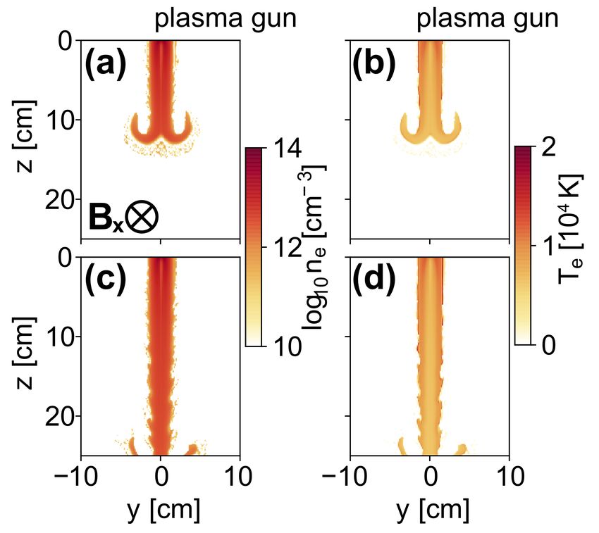
A&A 648, A81 (2021)

                                                                             observed in many YSOs (e.g., Gullbring et al. 1996; Safier
                                                                             1998; Bouvier et al. 2007; Cranmer 2009; Alencar et al. 2010;
                                                                             Stauffer et al. 2014).
                                                                                 The above models, however, cannot account for the episodic
                                                                             outbursts with large amplitude and long timescales such as those
                                                                             observed in EXor and FUor systems. The physical origin of the
                                                                             sudden large increase in mass accretion rates in YSOs is still
                                                                             largely debated in the literature, mainly as a result of the paucity
                                                                             of observed events and their rarity. Possible explanations for
                                                                             the FUor/EXor outbursts have been proposed in the literature.
Fig. 1. Cartoon of an accreting disc surrounding a young forming star.       The theoretical models explaining the origin of the outbursts can
Lines of the idealized star dipolar magnetic field are represented as        be roughly grouped in three main categories (Armitage 2019).
well, connecting the disc and star. Standard accretion inflows, following    A first class of models invokes a classical thermal instability
magnetic field lines, are represented as black droplets. Possible alterna-   (or secular instabilities; e.g., Armitage et al. 2001) that occur
tive inflow propagation across the magnetic field is represented as grey     in the accretion disc on a length scale of less than 1 AU (e.g.,
droplets.
                                                                             Bell & Lin 1994; see also Lasota 2001 for the case of dwarf
                                                                             nova outbursts). According to this model, the star-disc system
rates of 10−7 −10−6 M yr−1 , and emission line spectra. In addi-             is unable to accrete at a steady rate (as, for instance, in the mod-
tion, in the last decade a handful of objects have been found that           els discussed in the previous paragraph). As a result, the sys-
show outbursts with amplitude and timescales in between those                tem alternates phases in which the gas gradually accumulates at
of classical EXors and FUors (e.g., HBC 722 and V1647 Ori,                   the truncation radius, producing low accretion rates, to phases
Audard et al. 2014 and references therein). In the last decade               in which an instability (e.g., a thermal instability) may strongly
several multiwavelength sky surveys (e.g., Gaia1 , ASAS-SN2 ,                perturb the disc and, possibly, trigger a high accretion event.
Pan-STARSS3 , iPTF4 ) have significantly increased the number                A second class of models suggests that the episodic outbursts
of EXor/FUor candidates, which suggests that episodic accre-                 observed in EXor/FUor systems are triggered by a strong disc
tion is much more common behaviour for YSOs than previously                  perturbation by an object external to the star-disc system. The
thought.                                                                     perturbation may be due to the gravitational effects of a binary
    In recent years, significant effort has been made to describe            companion (Bonnell & Bastien 1992), or to the tidal effects by
the process of accretion of mass in young stellar objects (YSOs)             the migration of giant planets in the disc (Lodato & Clarke 2004;
through the development of accurate multidimensional magneto-                Nayakshin & Lodato 2012; Vorobyov & Basu 2005). In these
hydrodynamic (MHD) models. These theoretical and modelling                   cases, the disc can be affected by strong perturbations that trigger
studies have been very successful in describing the mass accre-              local instabilities (e.g., thermal instability) and lead to an event
tion in CTTSs and, in many cases, in compact objects as neutron              of high-accretion of mass. In a third class of models, the spo-
stars as well. These studies showed that the matter, in prox-                radic outbursts can be triggered by sudden changes in the stel-
imity of the disc truncation radius, may flow along magnetic                 lar magnetic activity (Armitage 1995, 2016; D’Angelo & Spruit
field lines of the magnetosphere (shown in Fig. 1) connecting                2012). Recent studies in the X-ray band have shown that the
star and disc (Hartmann 2008). Accretion would thus proceed                  activity cycle of young stars can be highly irregular and have
as sketched by the dark drops in Fig. 1, forming accretion fun-              sudden changes in the activity level (e.g., Sanz-Forcada et al.
nels that hit the stellar surface at high latitudes (e.g., Camenzind         2013; Coffaro et al. 2020); these changes are also characterized
1990; Koenigl 1991; Koldoba et al. 2002; Romanova et al. 2002,               by high amplitude in the level of magnetic activity that may per-
2003, 2004; Argiroffi et al. 2017). Another possibility is that              turb the disc and trigger high-accretion events. However, despite
accreting plasma may penetrate the magnetosphere in the equa-                significant theoretical and modelling efforts, to date none of the
torial plane, as sketched by the grey drops in Fig. 1, through               proposed models are able to provide a fully compelling descrip-
the development of Rayleigh-Taylor instability, forming thin                 tion of the EXor/FUor phenomenon. For instance it is still not
tongues of plasma accreting onto the central protostar (e.g.,                clear if EXors and FUors are different manifestations of the same
Arons & Lea 1976; Scharlemann 1978; Kulkarni & Romanova                      phenomenon or if they represent two different classes of objects.
2008). The above possibility was numerically investigated in                 We ask if they are triggered by the same physical mechanism
detail in Kulkarni & Romanova (2008), however, there are still               and occur in the same evolution phase of a young accreting
no sources based on astronomical observations supporting this                star.
hypothesis. Mass accretion can be even triggered by episodic                     From observations (see also Table 1 below) we can gather
perturbations of the accretion disc induced by an intense flar-              the following: values of the density, n ∼ 1012 −1014 cm−3 are rea-
ing activity occurring in proximity of the truncation radius (e.g.,          sonable, using as a starting guess the value in standard accre-
Orlando et al. 2011; Barbera et al. 2017; Colombo et al. 2019).              tion for CTTSs (see 5 × 1011 cm−3 , as in Bonito et al. 2014;
All these models describe the complex dynamics of magneto-                   Argiroffi et al. 2009). For the temperature, T ∼ 104 −106 K are
spheric accretion through an almost continuous formation and                 reasonable values (e.g., ZCMa emits in X-rays, see also val-
disruption of accretion streams, which may account for the                   ues for its jet in X-ray in Kastner et al. 2002; Argiroffi et al.
relatively short timescale (lasting from a few hours to sev-                 2007; Bonito et al. 2010a,b). The magnetic field of EXor-type
eral weeks) variability of mass accretion rates and luminosity               objects is still unknown owing to the low statistics of observa-
                                                                             tions for this class of objects. What is known is that the field
1
  https://sci.esa.int/web/gaia                                               in CTTSs, as measured on the surface of the stellar object, is,
2
  http://www.astronomy.ohio-state.edu/asassn/index.                          on average, of a few kG (Johns-Krull 2007; Johns-Krull et al.
shtml                                                                        2009; Donati et al. 2011a,b). Tens of G are thus reasonable val-
3
  https://panstarrs.stsci.edu/                                               ues for the B-field strength at the distance corresponding to the
4
  https://www.ptf.caltech.edu/iptf                                           disc truncation radius.

A81, page 2 of 10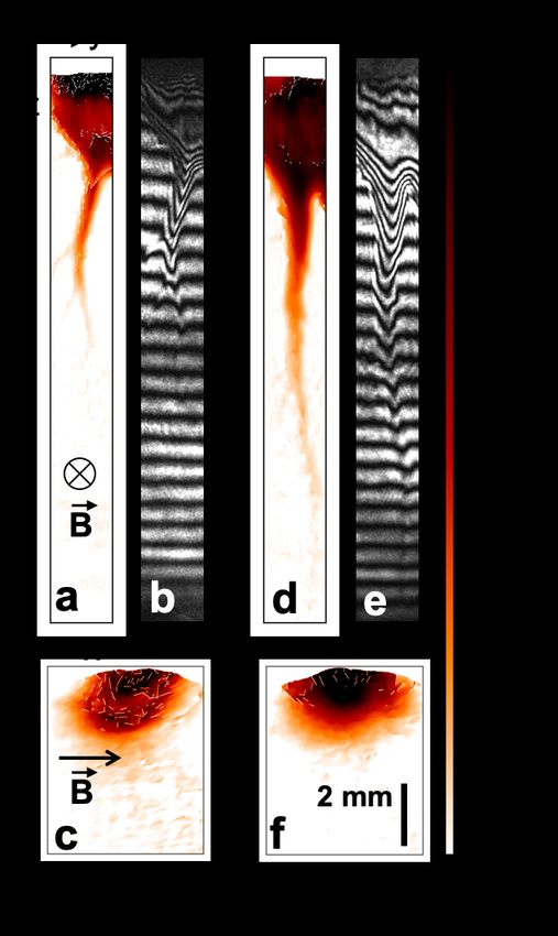
K. Burdonov et al.: Inferring magnetic field of EXor-type objects from scaled laboratory experiments

Table 1. Comparison and scalability between the laser-driven (PEARL)          knowledge we have of the laboratory flows to infer parameters
and plasma-gun driven (KROT) plasma streams, with the EXor accre-             of the EXor inflows that are not accessible in the present state
tion inflow investigated in Giannini et al. (2017).                           of the observational capabilities, among which is the magnetic
                                                                              field.
                        PEARL (i)           KROT             EXor                  Complementary to observations and numerical simulations
   Material            CF2 (Teflon)          CH2              H               of the processes, experiments conducted in the laboratory offer
                                                                              the possibility to gain further physical insight into the under-
   Z                         1               1.26               1             lying physics on a wide range of topics, from astrochem-
   A                       17.3              10.4             1.3             istry (Muñoz Caro & Escribano 2018) to plasma phenomena
   B [kG]                  135               0.45           0.105 •           (Remington et al. 2006). In contrast to computer modelling,
   L [cm]                   1.5              100           5 × 10¹¹           experiments involve real phenomena, which are not based on
   ne [cm−3 ]            5 × 10¹⁷            1013         5 × 10¹¹ ?          approximations, assumptions, and idealizations as the models
   ρ [g cm−3 ]          1.4 × 10⁻⁵       1.4 × 10⁻¹⁰      1.1 × 10⁻¹²         are. Experiments moreover include the full non-linearity of the
   T e [kK]                18.5               12             12 ?             processes. In contrast to observations, experiments conducted
   T i [kK]                18.5               12               12             in the laboratory can in general be run and re-run many times,
   Vflow [km s−1 ]         100                23             180 ?            while varying some input parameters (e.g., the plasma tempera-
   Cs [km s−1 ]             5.4               5.9             15.8            ture, ambient magnetic field, plasma density, and plasma com-
   VA [km s−1 ]            100               108              286             position) to assess their impact on the final observed plasma
   le [cm]               2 × 10⁻⁵            0.14               3             morphology and dynamics. However, the main and obvious dif-
   τcol e [ns]          3.8 × 10⁻⁴           3.3               70             ficulty is to assess how scalable, and hence relevant, such exper-
                                                                              iments are to astrophysical phenomena. Several studies have
   RLe [cm]             2.2 × 10⁻⁵       5.3 × 10⁻³       2.3 × 10⁻²
                                                                              looked in detail at this issue of scalability. This is discussed in
    fce [s−1 ]          3.8 × 10¹¹        1.3 × 10⁹        2.9 × 10⁸
                                                                              more detail in Sect. 4 below, but the general idea is to demon-
   li [cm]              2.8 × 10⁻⁵           0.12              4.1            strate that the main governing dimensional parameters of the lab-
   τcol i [ns]              0.1              400           4.8 × 10³          oratory and astrophysical plasmas are the same. This ensures that
   RLi [cm]              4 × 10⁻³            0.6               1.1            their dynamics is the same. The dimensional parameters allow us
    fci [s−1 ]          1.2 × 10⁷         8.3 × 10⁴        1.3 × 10⁵          to retrieve the scaling in time, space, density, velocity, magnetic
   M                       18.4               3.9             11.4            field, and so on between the two plasmas. Obviously, experi-
   Malf                      1                0.2              0.6            ments are conducted on plasmas that have much smaller extent
   τη [ns]              1.5 × 10³         1.2 × 10⁶       3.1 × 1025          (mm to m) than the astrophysical plasmas, but the duration of
   ReM                      10                27          1.1 × 10¹²          the events are also much shorter durations (ns to s). This has
   Re                   6.3 × 10³            650          4.7 × 10¹²          the advantage that the laboratory plasma dynamics can be usu-
   Pe                       35                4.7         9.7 × 10¹⁰          ally followed over a longer duration (when scaled) than what is
   Eu                       24                5.1              15             accessible to the astrophysical observations. A constraint how-
   β                    3.5 × 10⁻³       3.6 × 10⁻³       3.6 × 10⁻³          ever is that, as there is a self-organisation regulating the mag-
                                                                              netic field universally proportionally to the astrophysical system
Notes. (i) The primary parameters are noted in bold, while the numbers        size (Hillas 1984), usually the laboratory ambient magnetic field
in light are derived from these primary numbers. For the experimen-           has to be quite strong (10−100 G to MG), so that it can have an
tal streams, the primary numbers are directly measured or are deduced         effect on the plasma dynamics over the short spatial and tempo-
from simulations, as detailed in the text. For the EXor object, the B-field
                                                                              ral ranges at play.
value is an assumed one denoted with • symbol, and the parameters
reported by Giannini et al. (2017) are denoted with ? symbol.                      Laboratory plasmas can be produced by a wide variety of
                                                                              means, for example discharges, plasma guns, pinches, or lasers.
                                                                              In a series of previous works (Revet et al. 2017; Higginson et al.
    Our endeavour in this paper, since the parameters of that type            2017; Burdonov et al. 2020), we have already shown that, using
of phenomena are poorly known, is hence to improve our knowl-                 high-power lasers coupled to strong external magnetic field, we
edge of the parameters of the inflows that are at play. For this,             could generate plasmas that scale to accretion funnels of CTTSs,
we rely on laboratory experiments in which we produce differ-                 those that follow magnetic field lines, and that give rise to the
ent types of inflows propagating across magnetic field lines (as              standard observed accretion rates.
sketched in Fig. 1). The underlying idea is that, by showing that                  We explored the configuration in which plasma propagation
such inflow is possible, this gives weight to the possibility of              takes place across the magnetic field lines, that is in a configu-
having more accretion channels, and hence more mass accret-                   ration that would be akin to accretion in the equatorial plane, as
ing on the star, compared to having accretion relying solely on               sketched by the grey droplets in Fig. 1. The red dotted rectangle
processes at high latitudes at which the plasma is guided by the              in Fig. 1 indicates the situation modelled in this article. We note
magnetic field (Argiroffi et al. 2017). This would thus be a way              that such a configuration has already been investigated in a num-
to provide more mass, but the initiation of this process would still          ber of earlier studies performed using various plasma machines
rely on instabilities, as described above, which are not part of the          (Sucov et al. 1967; Bruneteau et al. 1970; Plechaty et al. 2013;
laboratory experiments. In particular, in the present work, we do             Tang et al. 2018; Khiar et al. 2019). In this work, we prolong
not discriminate between the conditions in which instabilities at             these previous efforts by generating plasmas that are scaled to the
the disc edge would occur. We merely show that plasma flows                   parameters of the massive accretion events which are our focus,
that can be scaled to what is known from EXor-type inflows can                as detailed below and in Table 1. This is done using two different
be measured and characterized well in the laboratory.                         methods and facilities, namely a plasma gun and a high-power
    We verify that these laboratory flows can be quantitatively               laser, the details of which are presented in Sect. 2. The use of
scaled to those that are inferred from EXor observations, as                  two types of plasma-generating devices is mainly done to have
detailed below and in Table 1. Then, we use the detailed                      two different sets of parameters (e.g., flow velocities, magnetic

                                                                                                                                A81, page 3 of 10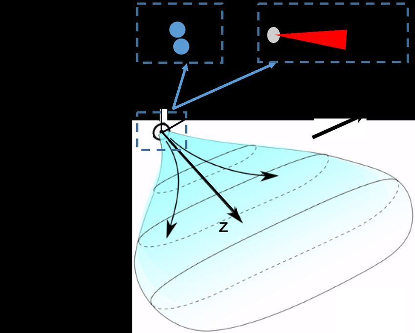
A&A 648, A81 (2021)

fields, and plasma densities), helping to constrain the parameters
that could be at play in EXors.
    We find that, first, consistent with previous studies, in both
cases efficient plasma propagation across the magnetic field lines
is possible, thus giving weight to the hypothesis of massive
accretion through the disc gap that was proposed by numeri-
cal simulations. Second, the laboratory streams parameters can
be scaled to those giving rise to the massive outbursts detailed
above, using the estimated parameters that can be retrieved from
the few observations we have of the latter. Doing this, an interest-
ing point is that the scaling of the laboratory magnetic field gives
a hint of the magnetic field that would be at play in the astro-
physical situation. As magnetic fields have not been primarily
derived from observations up to now, the laboratory experiments          Fig. 2. Schematic view of the experimental set-up. A plasma is gener-
are thus not only grounding the possibility of massive accretion         ated from a plasma gun or a laser-ablated Teflon (CF2 ) target. It expands
across magnetic field, as shown in Fig. 1, but further indicate in       into the vacuum (along z as the main expansion axis), which is embed-
which range of magnetic field this is possible.                          ded in a strong external magnetic field, orientated along x. Because of
    The paper is organized as follows. In Sect. 2, we describe           the imposed magnetization, the plasma is progressively flattened out
the facilities used for the laboratory modelling; in Sect. 3, we         along y, while it can flow along the magnetic field line (i.e. along x).
present the experimental results complemented by numerical               Hence, it progressively morphs into a ‘pancake’, as depicted.
simulations; in Sect. 4, we discuss the scalability of the labora-
tory experiment to the astrophysical phenomena of interest and
compare the laboratory parameters with the particular object rep-        Before being focussed, the beam was partially blocked by the
resenting the episodic accretion event; and in Sect. 5, we discuss       opaque screen that has a 10 mm opening gap centred with the
the results and draw our conclusions regarding the magnetic field        beam axis. As a consequence, the spot size on the target sur-
at play in the scaled EXor situations.                                   face had a quasi-rectangular shape (0.1 cm by 1 cm) delivering
                                                                         a laser intensity around 3 × 10¹⁰ W cm−2 . Optical interferometry
2. Laboratory experimental approach                                      imaging using a Mach-Zehnder scheme was used to diagnose
                                                                         the plasma stream propagation. The optical probing used a low-
In this section we present the two different facilities (plasma gun      energy (100 mJ), short-pulse beam (100 fs) to obtain a snapshot
and high-power laser), which we used to investigate the dynam-           of the plasma as it evolved. This was made simultaneously along
ics of plasma propagation across a strong external magnetic field.       two probing axes, namely y and z, to analyse the 3D nature of
In both cases, as illustrated in Fig. 2, we have a hot plasma that       the plasma flow. Such snapshots were captured at various times,
is generated either by the plasma gun or ablated by the high-            up to 108 ns with 10 ns step, relative to the laser-ablating laser
power laser from a solid target, which expands in a vacuum. The          impacting the target.
whole configuration is embedded in a magnetic field (aligned
with the x-axis) that is perpendicular to the main axis of the
                                                                         2.2. Using a plasma gun at the KROT facility
plasma expansion (z-axis). As illustrated by Fig. 2, as a con-
sequence of the interaction between the hot, expanding plasma            The large-scale (volume of 170 m3 ) KROT device
and the magnetic field, the plasma morphology, which is initially        (Aidakina et al. 2018) is the space plasma simulation chamber
conical and has an opening angle around 40◦ for the plasma gun           designed and constructed at the IAP RAS, Nizhny Novgorod
and around 30◦ (Revet 2018) for the laser, becomes flattened             (Russia). The chamber is equipped with a pulsed solenoid for
along the y-axis (i.e. that perpendicular to the magnetic field)         the magnetic field generation and a pulsed radio frequency
and stretched along the x-axis (i.e. that of the magnetic field). As     (RF) source of inductively coupled background plasma. The
shown in Sect. 3, this plasma structure propagates unimpeded             background plasma can be composed of argon or helium, and
across the magnetic field lines (i.e. in the direction of the z-axis).   has a maximum density of ne ∼ 1012 −1013 cm−3 ; the electron
                                                                         temperature reaches several eV. The magnetic field is set in a
2.1. Using the high-power laser facility PEARL                           mirror trap configuration, has a trap ratio R = 2.3, and a strength
                                                                         up to 450 G in the central cross section. Around the centre of
The high-power laser that is used to generate the expanding              the trap, the area with quasi-uniform field (i.e. it varies less than
plasma is at the PEARL laser facility (Lozhkarev et al. 2007;            10% within this region) has a length of about 1 m and diameter
Soloviev et al. 2017; Perevalov et al. 2020) located at the Insti-       not less than 1.3 m. The large volume of uniform magnetic field
tute of Applied Physics of the Russian Academy of Sciences               along and across field lines is a unique feature of the KROT
(IAP RAS), Nizhny Novgorod (Russia). The set-up is presented             plasma chamber.
in the Fig. 2. The laser pulse (3 J, 1 ns, 527 nm, normal inci-              The plasma flow was injected into the vacuum at the resid-
dence) irradiated the surface of a thick, solid CF2 target that          ual air pressure p0 ∼ 3−50 µ Torr and propagated in the ambient
has its normal orientated along the z-axis. The laser, ablating          B-field having strength from 45 to 450 G. The overall set-up,
the surface target material, induced the expansion of a plasma           illustrated in Fig. 2, is similar to that of the high-power
stream into the vacuum, along the z-axis and perpendicular to            laser experiment. The plasma was generated by a “cable gun”
the externally imposed B-field of 1.35 × 10⁵ G). The magnetic            made of a 50 Ohm coaxial cable with a polyethylene insula-
field was created by a Helmholtz coil that maintained a spatially        tor (Gushchin et al. 2018; Korobkov et al. 2019). The gun was
(∼2 cm) and temporally (∼1 µs) constant field over the scales            installed at the centre of the area of the quasi-uniform magnetic
of the experiment (1 cm and 100 ns). The initial laser beam had          field. The plasma flow was induced via high-voltage surface
a flat-top circular-shaped spatial profile with 100 mm diameter.         breakdown on the insulator, with subsequent plasma acceleration
A81, page 4 of 10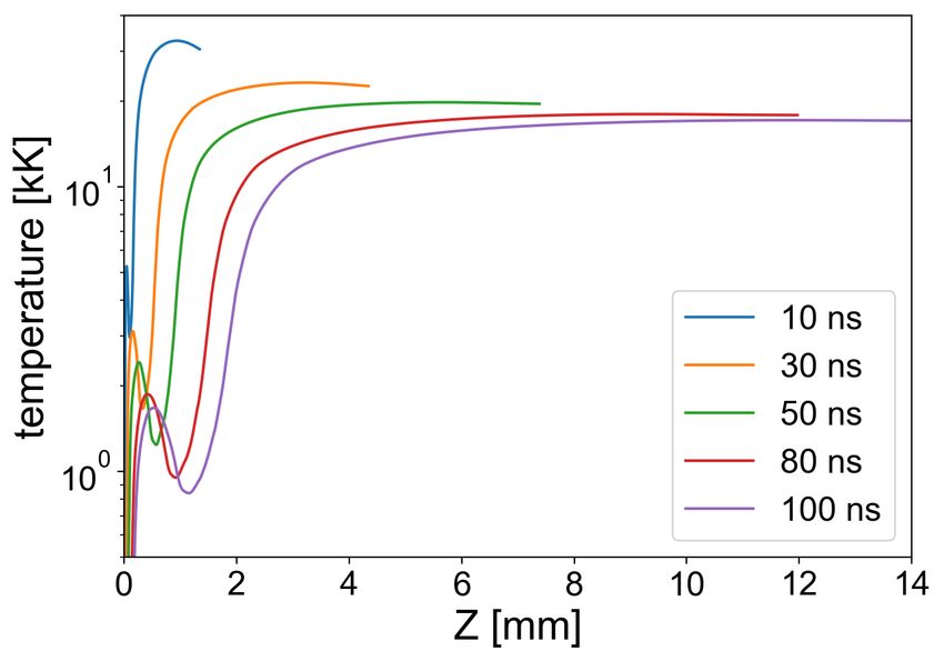
K. Burdonov et al.: Inferring magnetic field of EXor-type objects from scaled laboratory experiments

by the Ampere force (Marshall 1960). The outer diameter of
the gun was 10 mm and its operating voltages and currents were
around 5 kV and 4 kA, respectively. The current pulse duration
was about 15 µs at its base, while the current rise time was
7 µs.
    Several diagnostics were used to measure the plasma param-
eters (Gushchin et al. 2018). The self-emission from the plasma
stream was recorded, using a 4Picos fast shutter camera, along
two directions, parallel and perpendicular to the B-field lines
axis. The snapshots were taken from 0 µs to 30 µs after the gun
discharge ignition with 1 µs step. The local plasma density ne
and electron temperature T e values were measured using double
electric probes immersed into the plasma stream. The plasma
density, averaged over the stream cross section, was measured
using a microwave interferometer with an operating frequency
of 37.5 GHz and from the cut-off of a probing microwave sig-
nal with the same frequency. Local magnetic disturbances were
measured by a set of identical B-dot probes. The diamagnetic
effect in the stream moving into the ambient magnetic field
was used as an independent method for diagnosing the plasma
parameters (i.e. its density and temperature).

3. Laboratory plasma measurements
In this section we present the results of the laboratory experi-
ments performed as presented in the previous section, comple-
mented by numerical modelling. Despite different spatial and
temporal scales, in both cases the plasma flow demonstrated sim-
ilar propagating features. The values of the plasma flow veloc-
ities, densities, and temperatures, presented in this section, are
used in the following section to link the laboratory plasma with
the astrophysical phenomena of interest.

3.1. Measurements of the high-power laser generated
     plasma density and velocity
Figure 3 shows the measurements of the laser-generated plasma
flow. The fact that we irradiated a large surface of the target
                                                                        Fig. 3. Line-integrated, 2D projections of the electron density as mea-
induced a complex, fragmented morphology of the plasma, sim-            sured, 58 ns after the laser impact onto the target, (a) in the yz and (c)
ilar to what has already been observed in current-driven plasma         xz-planes. Panel b: a raw interferometry image for the yz-plane for bet-
flows from thick rods (Ivanov 2006). In this work we do not             ter illustration. Panels d–f: same at 108 ns after the laser impact onto
focus on characterizing the plasma structure, but rather focus on       the target. The projections in the two orthogonal planes are measured
the global parameter (velocity, density, and temperature) of the        simultaneously.
central part of the expanding plasma. From Fig. 3, we verify that
the global morphology of the plasma is similar to that illustrated
in Fig. 2; that is, the plasma can spread in the x-axis, while it is    simulations to retrieve the temperature of the propagating plasma
pinched along the y-axis, resulting in an overall pancake shape.        pancake. For this, we use the Lagrangian 1D hydrodynamic code
The electron density value of the propagating flow at the dis-          ESTHER (Colombier et al. 2005). As shown schematically in
tance of about 5 mm from the target surface was of the order of         Fig. 2, the plasma flow is constrained in the shape of a pan-
5 × 1017 cm−3 .                                                         cake by the external magnetic field, that is it is flattened in the yz
     The temporal evolution of the tip of the plasma flow is shown      plane, but expands laterally in the xz plane. So, in the xz plane,
in Fig. 4. The tip position was defined as corresponding to             the situation is 1D since the plasma is constrained by the B-field.
5 × 1016 cm−2 in the 2D projection of the electron density in the       In the xz plane, the situation is 2D, but since the radial size of
yz-plane. Since the width of the plasma pancake (in the xz plane)       the pancake expansion front is large, locally, the situation can
is around 0.3 cm, that threshold thus corresponds to a volumetric       be approximated in 1D. Hence, we simulate a central line of the
density around 1017 cm−3 . We observe that the tip of the plasma        expanding plasma with ESTHER. The simulation does not treat
has a constant velocity of around 100 km s−1 .                          the background magnetic field; the justification for this is that
                                                                        within its expansion, as it propagates the plasma expels the mag-
3.2. Simulations of the high-power laser generated plasma               netic field (Khiar et al. 2019). This code solves, according to a
     temperature                                                        Lagrangian scheme, the fluid equations for the conservation of
                                                                        mass, momentum, and energy. The target material is described
Since we could not directly measure the temperature of the              by the Bushman-Lomonosov-Fortov (BLF) multi-phase equa-
plasma generated by the high-power laser, we rely on numerical          tion of state spanning a large range of density and temperature
                                                                                                                               A81, page 5 of 10
A&A 648, A81 (2021)
Fig. 4. Temporal evolution of the tip of the laser-generated plasma flow,
as retrieved from images as those shown in Fig. 3 (full dots) and as sim-
ulated by the ESTHER code (empty stars). The dashed line corresponds
to an average velocity of 100 km s−1 .
Fig. 5. Temperature distribution, over time, of a laser-generated plasma
flow, as simulated with the ESTHER code, and using similar parameters
as the experimental parameters (see text).
from hot plasma to cold condensed matter. ESTHER is a single-
temperature code, i.e. T e = T i . We use this code since it specif-
ically allows us to simulate the transition to plasma of a solid
under the impact of a low intensity laser (Colombier et al. 2005),
which has an intensity of the order of 1010 W cm−2 . Since we
cannot simulate a composite material as that used in the exper-
iment, a pure carbon target was simulated. Figure 5 represents
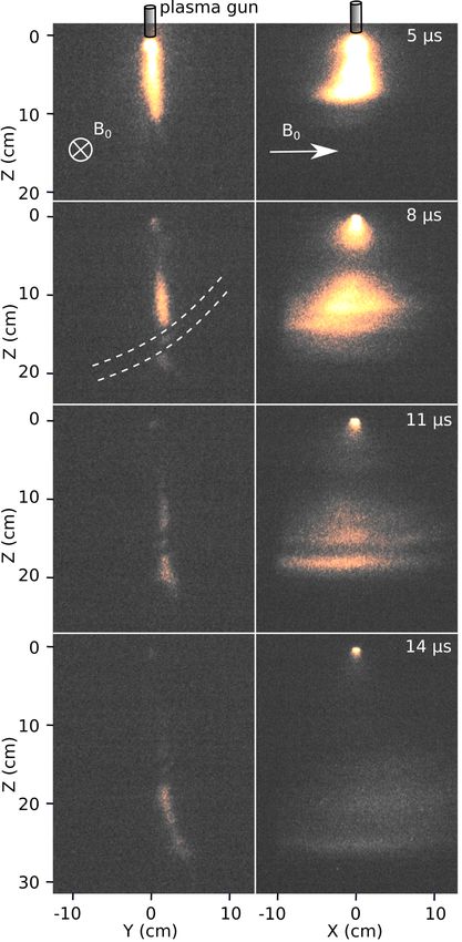
the plasma temperature distribution from the target surface up to Fig. 6. Images of the self-emission of the plasma-gun generated flow
tens mm along the main expansion axis (the z-axis, see Fig. 2) (in the case in which the applied magnetic field strength is 450 G), at
various times after the start of injection (as indicated) and in the yz (left
at specific times 10 ns, 30 ns, 50 ns, 80 ns, and 100 ns after the column) and xz (right column) planes. The dashed lines denote the loca-
impact of a laser pulse with 3 × 10¹⁰ W cm−2 , which has a Gaus- tion of a cable line placed between the plasma flow and the observation
sian temporal shape and a 1 ns FWHM duration. We observe camera, hence locally obscuring the flow.
that the plasma stabilizes around a temperature of ∼17−20 kK
far from the target (i.e. at distances of ∼6−12 mm and times of
∼50−100 ns). The fact that the temperature is high only at the pancake thickness was about δy = 2 cm. This pancake-shaped
head of the expanding plasma is related to the fact that the laser plasma flow propagates with its main axis along z (see Fig. 2),
energy is low, and hence only a thin layer on the target surface that is perpendicularly to the average direction of the magnetic
can be ablated and be at high temperature. The position of the field, up to 50−70 cm from the injection point and with almost
tip in the simulations, presented in the Fig. 4, defined at the dis- constant velocity (around 23 ± 1) km s−1 (see Fig. 7). The tip
tance from the target surface, where the electron density equals position was defined as the position at which the plasma lumi-
to 1 × 1017 cm−3 . nosity was at the level of ∼0.25 from the averaged, which cor-
responds to the electron plasma density of the order of several
3.3. Measurement of the plasma gun generated plasma 1012 cm−3 . Additional features of the plasma flow dynamics in
a transverse magnetic field were the presence of a twist of the
As can be seen in Fig. 6, the plasma gun-generated flow demon- stream in the direction of ion gyration (see Fig. 6, on the left)
strates the same topological features as the laser-generated flow. and the development of an observed transverse fragmentation of
Without a magnetic field, the plasma expanded into a cone that the flow (see Fig. 6, on the right).
has an opening angle of (37 ± 3)◦ . In the presence of the mag- The measured electron density was ne ∼ 1013 cm−3 inside
netic field, the plasma flow was transformed into a pancake the pancake and above 1014 cm−3 near to the injection point.
structure, similar as that of the laser-generated plasma (compare The electron temperature was up to ∼46 kK during the gun dis-
Figs. 3 and 6). For magnetic field strengths higher than 100 G, charge at the time of maximum current (around 7 µs after the
the pancake thickness was inversely proportional to the magnetic start of injection). Later, at the stage of the pancake plasma free
field strength. For the maximum magnetic field, B0 = 450 G, the expansion, the electron temperature was around 12 kK. The level
A81, page 6 of 10K. Burdonov et al.: Inferring magnetic field of EXor-type objects from scaled laboratory experiments
Fig. 7. Temporal evolution of the tip of the plasma gun-generated flow
(in the case in which the applied magnetic field strength is 450 G), as
retrieved from images as those shown in Fig. 6 (full dots) and as simu-
lated by the GORGON code (empty stars). The dashed line corresponds
to an average velocity of 22.7 km s−1 .
of diamagnetic disturbances inside the pancake was not higher
than several G and could be attributed to the thermal diamag-
netism of the plasma.
The presence of an optional background argon plasma, Fig. 8. Three-dimensional MHD simulations of the plasma gun gener-
which has a density of up to 1012 cm−3 and temperature ated flow performed with the GORGON code. Two-dimensional distri-
T e ∼ 12 kK, affected neither the observed dynamics of plasma butions of the plasma in yz-plane, passing through the middle of the 3D
flow nor the measured plasma parameters for the same range of flow, are shown. Panels a and b: are at t = 6 µs, while panels c and d:
magnetic field strengths. The formation of the observed pancake are at t = 12 µs. The plasma gun is at the top, like in the experiment (see
structure was a persistent physical effect, which was insensitive Fig. 6). The electron number densities [cm−3 ] are shown on the left in
to the presence of a background plasma with an electron density logarithmic scale, while the electron temperatures [Kelvins] are on the
right. The applied magnetic field is Bx = 450 G, directed out of plane.
comparable to that of the plasma flow.
3.4. Simulations of the plasma gun generated flow temperature and are thus not shown in this work. Besides, the
simulation confirms the characterization of the plasma param-
We used the resistive, single-fluid, bi-temperature and highly eter from the experiment: the electron density of the stream is
parallel code GORGON (Ciardi et al. 2007, 2013) to perform 3D around 1013 cm−3 , the electron temperature is around 12 kK, and
MHD simulations of the plasma gun generated flow. Since the the velocity of the plasma flow is more than 20 km s−1 . The
laboratory measurements are performed with probes inserted in criteria to define the tip position, presented in the Fig. 7, is
the flow, the simulations can be used as a check that the measured 2.0 × 1012 cm−3 in the yz-plane sliced at x = 0.
parameters match those of the (simulated) unperturbed flow. Moreover, by comparing the cases with and without back-
The simulation box is defined by a uniform Cartesian grid ground gas (not shown here), we see that the pancake structure
of dimension 20 × 20 × 30 cm3 and the number of cells equals is almost the same, confirming that the effect of a background
to 160 × 160 × 240. The spatial resolution is homogeneous, its can be neglected, as found in the plasma gun experiments.
value is d x = dy = dz = 1.25 mm, and the simulation lasts for
30 µs.
The plasma (CH2 ) is injected from the centre of the bound- 4. Scaling of the laboratory plasmas to EXor
ary at z = 0 with the same diameter as the KROT injector. objects
The initial density is 3 × 1013 cm−3 , the velocity is 25 km s−1
(with 40◦ cone angle), and the temperature is ∼46 kK. A uniform Now that we detailed the parameters of the laboratory propagat-
B-field along the x-direction is applied, with a series of strength ing plasmas, we describe how they can be quantitatively scaled
(i.e. Bx = 56/112/225/450 G) and cases with and without back- to those of the EXors accreting inflows. This section describes
ground cold helium gas with a number density of 1012 cm−3 are that scalability approach used for the comparison of the labo-
compared. ratory plasma with the astrophysical plasma. For the latter, we
The simulation results for Bx = 450 G are shown in Fig. 8. focus on the estimated parameters of the incoming stream before
Electron number densities are on the left, while electron tem- its impact on the surface of the star, as derived in Giannini et al.
peratures are on the right. The tongue structures seen at the (2017).
tip of the plasma jet in Fig. 8 originate from the initialization
of the simulation, namely from how we inject plasma from the 4.1. Principle of the scalability
boundary of the simulation box. These structures are not impor-
tant for plasma dynamics and we do not observe well-developed The scalability between the laboratory plasma and the astrophys-
Rayleigh-Taylor instability or the Kelvin-Helmholtz instability ical plasma is based on the approach proposed in the works by
within the timescale of interest in our simulations. Ryutov (Ryutov et al. 1999, 2000; Ryutov 2018). The “Euler
First and foremost, we observe that the GORGON simula- similarity” is based on two scaling quantities: the Euler num-
tion reproduces the pancake structure from the KROT exper- ber (Eu = V(ρ/p)1/2 , here and below the formulas are presented
iment and has a stable width of ∼3 cm. The results in the for cgs units) and the plasma beta (β = 8π p/B2 ), where V is the
xz-plane merely display a homogeneous plasma in density and flow velocity, ρ is the mass density, B is the magnetic field, and
A81, page 7 of 10A&A 648, A81 (2021)
p = kB (ni T i + ne T e ) is the thermal pressure; kB is the Boltzmann
constant and ni,e and T i,e are the number densities and tempera-
tures of the ions and electrons, respectively. When matching for
two different systems, it can be shown that these two systems are
scaled to each other and evolve identically.
The Euler similarity holds and allows us to use ideal MHD
equations if dissipative processes, which might affect the fluid
dynamics, are neglected. The Reynolds number (the ratio of the
inertial force to the viscous force) is responsible for the viscous
dissipation, the magnetic Reynolds number (the ratio of the con-
vection over Ohmic dissipation) for the resistive diffusion, and
the Peclet number (the ratio of heat convection to the heat con-
duction) for the thermal conduction. All these parameters should
be higher than 1 to meet the required conditions.
We note that for the episodic accretion EXor events, not all
the parameters necessary for the comparison with the laboratory
systems are known. The analysis of the astronomical observa-
tions allows us to estimate the plasma densities, temperatures,
and characteristic velocities of the streams. However, as men-
tioned in Sect. 1, the magnetic field of the involved protostars
is not known. Some works report estimations of kilogauss lev-
els (Donati et al. 2005, FU Ori; Green et al. 2013, HBC 722)
while for the EXors the magnetic field is supposed to be weaker
(Audard et al. 2014), of the order of hundred G. One of the
objectives of the present work is to use the scalability to the
laboratory flows to estimate the possible values of the B-field
strength of the EXor objects.
4.2. Comparison of the laboratory flows to the accretion
events of EXor objects
In the paper (Giannini et al. 2017), the parameters of the
observed episodic accretion event of a particular EXor object
were presented. The typical densities of the accretion stream in
the rising/peak phase range from 4 × 1011 cm−3 to 6 × 1011 cm−3 , Fig. 9. Panel a: correlation between the magnetic field and the β. The
the temperatures range from 9 kK to 15 kK and the stream veloc- grey area represents the range of EXor parameters, the dot-dashed ver-
ities range from tens to hundreds km s−1 . But no information tical line indicates the laser-driven flow β, the dotted line indicates the
about the B-field strength can be retrieved from such observa- plasma gun-driven flow β, and the black point represents the parame-
tions. ters of the EXor used in the Table 1. Panel b: same for the correlation
Figure 9 represents the phase-space of the possible plasma between the stream velocity and the Euler number.
beta and Euler number of the considered EXor object, depend-
ing on the B-field strength and the stream velocity propagation, √
respectively. The grey areas correspond to the estimated range the adiabatic index); VA is the Alfven velocity (VA = B/ 4πni mi ,
of parameters for accreting inflows in EXor objects. The dot- where ni is the ion density and mi is the ion mass); τcol e is the
dashed vertical lines denote the plasma beta corresponding to the electron collision time (Braginskii 1965 at p. 215); le = Vth e τcol e
laser-driven flow, while the dotted lines correspond to the plasma is the collisional electron mean free path, where Vth e is the elec-
gun-driven flow. From the Fig. 9a we see that both the laser- tron thermal velocity (Richardson 2019 p. 29); RLe is the elec-
driven flow and the plasma gun-driven flow scale to the EXor B- tron Larmor radius, fce is the electron gyrofrequency; τcol i is
field in the range from ∼85 to ∼135 G. Figure 9b shows that the the ion collision time (Braginskii 1965 at p. 215); li = Vth i τcol i is
EXor accreting inflow velocity ranging from 260 to 330 km s−1 the collisional ion mean free path, where Vth e is the ion thermal
scales to the laser-driven flow and from 55 to 70 km s−1 to the velocity (Richardson 2019 p. 29); RLi is the ion Larmor radius,
plasma gun-driven flow. The black points in the figure indicate fci is the ion gyrofrequency; M = Vflow /Cs is the Mach number;
the typical averaged parameters of EXor used in Table 1; B-field Malf is the Alfven Mach number (Malf = V/VA ); τη is the mag-
is assumed to be 105 G.
netic diffusion time (τη = L2 /η, where η is the magnetic diffusiv-
In the comparative Table 1, the parameters of the laser and
ity (Ryutov et al. 2000 p. 467); ReM is the magnetic Reynolds
plasma gun-driven laboratory streams and the considered EXor
accretion stream (denoted with the black point in Fig. 9) are number (ReM = LV/η); Re is the Reynolds number (Re = LV/ν,
listed. All parameters are calculated for plasma inside the prop- where ν is the kinematic viscosity (Ryutov et al. 1999 p. 826);
agating stream; no shocks are considerable. The symbols in Pe is the Peclet number (Pe = LV/χ), where χ is the thermal dif-
Table 1 are as follows: Z is the charge state; A is the mass fusivity (Ryutov et al. 1999 p. 824); Eu is the Euler number; and
number; B is the magnetic field; L is the spatial scale; ne is the β is the plasma beta.
electron density; ρ is the mass density; T e is the electron temper- The laboratory plasma streams are characterized by three dif-
ature; T i is the ion temperature; Vflow is the stream velocity; Cs is ferent scales along the x, y, and z axes, which are around 0.3,
the sound velocity (Cs = (γkB (ni T i + ne T e )/ρ)1/2 , where γ = 5/3 is 0.1, and 1.5 cm for the laser-driven flow and 10, 3, and 100 cm
A81, page 8 of 10K. Burdonov et al.: Inferring magnetic field of EXor-type objects from scaled laboratory experiments
for the plasma gun-driven flow. The spatial scale along the z-axis stream. The fact that the value of the magnetic field, as inferred
was used in Table 1. from the scaling, for FU Orionis is of the same order as that
As shown in Table 1, the plasma beta values match the three inferred for the EXor is consistent with the most updated knowl-
considered flows perfectly and the Euler numbers are of the edge (Audard et al. 2014). This fact supports the idea of identi-
same order, however these values are not exactly the same. We cal accretion mechanisms being at play in the EXor and FUor
have two laboratory flows that can each be scaled to the EXor objects.
inflow and can reasonably correspond to a range of parameters
of the latter. Therefore, we can examine what exactly matching
the EXor inflow to either the laser or plasma gun-driven flows 5. Discussion and conclusions
would entail, while keeping the temperature, density, and B-field Eruptive variables of the EXor/FUor type displaying powerful
of the EXor inflow the same as in Table 1. This leads to, for the outbursts are still rarely observed and hence their characteristics
EXor Vflow = 290 km s−1 , Eu = 24, which perfectly fits the laser- are still not well known. Apart from their interesting character-
driven flow case. Similarly, for the EXor Vflow = 62 km s−1 , we istics, these objects could be a possible solution for the well-
have Eu = 5.1, which corresponds to the plasma-gun driven case. known the Luminosity Problem if it would confirm that they
Following Ryutov’s analysis, we extracted the scaling factors represent a more common behaviour for YSOs than previously
in space, density, and velocity between the EXor and laboratory thought. Indeed, the luminosity of YSOs is lower of about an
flows. This yields the following factors, denoted with “P” and order of magnitude than if the accretion proceeds at the accretion
“K” for the laser-driven (PEARL) and plasma gun-driven flows rates predicted by the standard steady-state collapse model of
(KROT), respectively. The spatial scaling parameters are as fol- Shu (1977). This problem, originally described by Kenyon et al.
lows: (1990), has been observationally confirmed by the Spitzer satel-
lite survey of a number of star formation regions (Evans et al.
rast 5 × 10⁶ [km]
aP = = = 3.3 × 10¹¹ , 2009).
rP lab 1.5 [cm] We attempted to use measurements of laboratory plasma
rast 5 × 10⁶ [km] flows to complement our knowledge of these objects and in par-
aK = = = 5 × 10⁹ . ticular of the magnetic field environment in which they could
rK lab 100 [cm]
take place. For this, we demonstrated the analogy between
The density scaling parameters are written as the accretion inflows recorded during intense outbursts of
EXor/FUor objects and the laboratory plasmas created at two
ρast 1.1 × 10⁻¹² [g cm−3 ] facilities, PEARL (high power laser) and KROT (plasma gun
bP = = = 7.9 × 10⁻⁸ ,
ρP lab 1.4 × 10⁻⁵ [g cm−3 ] injector), which have different scales and plasma parameters.
ρast 1.1 × 10⁻¹² [g cm−3 ] The laboratory experiments demonstrate that effective prop-
bK = = = 7.9 × 10⁻³ , agation of plasma is possible across B-field, which supports the
ρK lab 1.4 × 10⁻¹⁰ [g cm−3 ] proposed scenario of matter accretion not only along the mag-
and the velocity scaling parameters are netic field lines but also across them (see Fig. 1). This effect can
be a candidate to explain the origin of the high accretion rates of
Vast 290 [km s−1 ] the EXor/FUor objects in comparison with standard accretion in
cP = = = 2.9, CTTS.
VP lab 100 [km s−1 ]
The demonstrated scalability between the two laboratory
Vast 62 [km s−1 ] plasmas and the astrophysical plasma allows us to access
cK = = = 2.7. unknown parameters of the astrophysical system, such as the
VK lab 23 [km s−1 ]
magnetic field. In particular, we have shown that we could derive
Based on these factors, the temporal scaling tast = (aP /cP )tP lab the magnetic field strengths this way for the EXor object detailed
gives that 100 ns of the laser-driven flow is equivalent to around in Giannini et al. (2017) (i.e. around 100 G) or for the FU Orionis
1.1 × 10¹³ ns (∼3 h) of the √ astrophysical flow. The magnetic star (Labdon et al. 2021) (i.e. around 200 G) are inconsistence
field scaling Bast = BP lab cP bP means that 135 kG in the laser- with the most up-to-date understanding of such stellar objects.
driven flow case corresponds to ∼110 G in the case of the EXor We note that the scaled magnetic field we infer for the astro-
object. For the plasma gun-driven case tast = (aK /cK )tK lab gives physical situations corresponds to average values that would be
that 25 µs is equivalent to around 9.3 √× 108 µs (∼13 h) and for experienced by accretion streams as they propagate from the disc
450 G in the laboratory Bast = BK lab cK bK gives ∼105 G for the to the star. Lower magnetic fields are thus expected closer to the
astrophysical case. disc and correspondingly higher fields would be expected at the
The similarity detailed above was made between the exper- star surface. Since we find average values for the in-stream mag-
iments and the EXor object detailed in Giannini et al. (2017). netic field of a few hundreds of G, fields in the kG range at the
We find that a similarly good scalability can be found between star surface, as found in CTTSs, would thus be reasonable. This
our experimental measurements and the FU Orionis star, whose points out that EXor/FUor-objects might not be out of the norm,
characterization was recently improved by Labdon et al. (2021). but rather represent particular episodic behaviour of otherwise
In that case, taking the temperature value to be around 2 kK at standard CTTSs.
the FU Orionis truncation radius, and assuming an averaged den- Future perspectives to refine the parameters of EXor accre-
sity of ∼1013 cm−3 and a velocity of ∼120 km s−1 for the accre- tion streams include low-energy observations possibly tuned to
tion stream, we find that this stream scales that produced by the more extreme cases that could then be compared with laboratory
high-power laser produced plasma (detailed in Table 1) for a experiments tuned in the appropriate regime. Laboratory exper-
∼200 G magnetic field strength value in the astrophysical case. iments and numerical simulations are crucial for predictions
If the matching is done with the plasma-gun generated plasma, on current and future high-energy observations (e.g., eROSITA,
we find that this is possible for a magnetic field of 200 G, a den- XRISM, and Athena) for parameters on which no constraints can
sity of 1013 cm−3 and a velocity of 30 km s−1 for the accretion be evaluated with current data. The topic discussed in this work
A81, page 9 of 10A&A 648, A81 (2021)
is also timely from the perspective of possible future big data Camenzind, M. 1990, Rev. Mod. Astron., 3, 234
surveys, which will allow us to collect multi-band observations. Ciardi, A., Lebedev, S., Frank, A., et al. 2007, Phys. Plasmas, 14, 056501
These include Rubin LSST in the low-energy regime along with Ciardi, A., Vinci, T., Fuchs, J., et al. 2013, Phys. Rev. Lett., 110, 025002
Coffaro, M., Stelzer, B., Orlando, S., et al. 2020, A&A, 636, A49
eROSITA, XRISM, and Athena in the high-energy regime. Pos- Colombier, J. P., Combis, P., Bonneau, F., Le Harzic, R., & Audouard, E. 2005,
sible explanations of the lack of high statistics in the number of Phys. Rev. B, 71, 165406
observed objects with accretion outbursts such as EXors could Colombo, S., Orlando, S., Peres, G., et al. 2019, A&A, 624, A50
also be helped by future observational campaigns (such as the Cranmer, S. R. 2009, ApJ, 706, 824
D’Angelo, C. R., & Spruit, H. C. 2012, MNRAS, 420, 416
Rubin LSST ten-year survey). First, these objects could be very Donati, J.-F., Paletou, F., Bouvier, J., & Ferreira, J. 2005, Nature, 438, 466
common, but we observed just a few of them because we need Donati, J.-F., Bouvier, J., Walter, F. M., et al. 2011a, MNRAS, 412, 2454
a proper cadence of observing strategy; see discussion on a pos- Donati, J.-F., Gregory, S. G., Montmerle, T., et al. 2011b, MNRAS, 417,
sible cadence for variability in accreting stars (i.e. CTTSs and 1747
EXors) with Rubin LSST in Bonito et al. (2018). Second, the Evans, N. J., II, Dunham, M. M., Jørgensen, J. K., et al. 2009, ApJS, 181, 321
Giannini, T., Antoniucci, S., Lorenzetti, D., et al. 2017, ApJ, 839, 112
range of parameters that trigger the burst is too small. Numerical Green, J. D., Robertson, P., Baek, G., et al. 2013, ApJ, 764, 22
simulations and laboratory experiments (as those described here) Gullbring, E., Barwig, H., Chen, P. S., Gahm, G. F., & Bao, M. X. 1996, A&A,
are ideal to perform a wide exploration of the parameter space. 307, 791
We plan to investigate these points with multi-band surveys in Gushchin, M. E., Korobkov, S. V., Terekhin, V. A., et al. 2018, JETP Lett., 108,
391
the near future and an active project to monitor these objects in Hartmann, L. 2008, Accretion Processes in Star Formation (Cambridge:
the optical band and in X-rays with Rubin LSST and eROSITA, Cambridge University Press)
respectively, is ongoing5 . Higginson, D., Revet, G., Khiar, B., et al. 2017, High Energy Density Phys., 23,
48
Hillas, A. M. 1984, ARA&A, 22, 425
Acknowledgements. This work was supported by funding from the European Ivanov, V. V., et al. 2006, Phys. Plasmas, 13, 012704
Research Council (ERC) under the European Unions Horizon 2020 research Johns-Krull, C. M. 2007, ApJ, 664, 975
and innovation program (Grant Agreement No. 787539). The experiments at the Johns-Krull, C. M., Greene, T. P., Doppmann, G. W., & Covey, K. R. 2009, ApJ,
KROT facility were supported by the Russian Foundation for Basic Research 700, 1440
(RFBR) in the frame of project No. 18-29-21029, and Unique Scientific Facility Kastner, J. H., Huenemoerder, D. P., Schulz, N. S., Canizares, C. R., &
“Complex of Large-Scale Geophysical Facilities (KKGS)” was used. The exper- Weintraub, D. A. 2002, ApJ, 567, 434
iments at the PEARL facility were supported by the Russian Science Founda- Kenyon, S. J., Hartmann, L. W., Strom, K. M., & Strom, S. E. 1990, AJ, 99, 869
tion (RSF) in the frame of project No. 20-12-00395. The work of JIHT RAS Khiar, B., Revet, G., Ciardi, A., et al. 2019, Phys. Rev. Lett., 123, 205001
team was done in the frame of the State Assignment (topic No. 075-00892- Koenigl, A. 1991, ApJ, 370, L39
20-00) and partially funded by Russian Foundation for Basic Research (grant Koldoba, A. V., Romanova, M. M., Ustyugova, G. V., & Lovelace, R. V. E. 2002,
No. 18-29-21013). This work was partly done within the LABEX Plas@Par, ApJ, 576, L53
the DIM ACAV funded by the Region Ile-de-France, and supported by Grant Korobkov, S. V., Gushchin, M. E., Gundorin, V. I., et al. 2019, Tech. Phys. Lett.,
No. 11-IDEX- 0004-02 from ANR (France). Part of the experimental system is 45, 228
covered by a patent (1000183285, 2013, INPI-France). The research leading to Kulkarni, A. K., & Romanova, M. M. 2008, MNRAS, 386, 673
these results is supported by Extreme Light Infrastructure Nuclear Physics (ELI- Labdon, A., Kraus, S., Davies, C. L., et al. 2021, A&A, 646, A102
NP) Phase II, a project co-financed by the Romanian Government and European Lasota, J.-P. 2001, New Astron. Rev., 45, 449
Union through the European Regional Development Fund, and by the project Lodato, G., & Clarke, C. J. 2004, MNRAS, 353, 841
ELI-RO-2020-23 funded by IFA (Romania). RB and TG acknowledge support Lozhkarev, V. V., Freidman, G. I., Ginzburg, V. N., et al. 2007, Laser Phys. Lett.,
from the project PRIN-INAF 2019 “Spectroscopically Tracing the Disk Disper- 4, 421
sal Evolution”. SO acknowledges partial support from INAF-Osservatorio Astro- Marshall, J. 1960, Phys. Fluids, 3, 134
nomico di Palermo. Muñoz Caro, G. M., & Escribano, R. 2018, Laboratory Astrophysics (New York:
Springer)
Nayakshin, S., & Lodato, G. 2012, MNRAS, 426, 70
References Orlando, S., Reale, F., Peres, G., & Mignone, A. 2011, MNRAS, 415, 3380
Perevalov, S. E., Burdonov, K. F., Kotov, A. V., et al. 2020, Plasma Phys. Control.
Aidakina, N., Galka, A., Gundorin, V., et al. 2018, Geomagn. Aerono., 58, 314 Fusion, 62, 094004
Alencar, S. H. P., Teixeira, P. S., Guimarães, M. M., et al. 2010, A&A, 519, A88 Plechaty, C., Presura, R., & Esaulov, A. A. 2013, Phys. Rev. Lett., 111, 185002
Argiroffi, C., Maggio, A., & Peres, G. 2007, A&A, 465, L5 Remington, B. A., Drake, R. P., & Ryutov, D. D. 2006, Rev. Mod. Phys., 78, 755
Argiroffi, C., Maggio, A., Peres, G., et al. 2009, A&A, 507, 939 Revet, G. 2018, Theses, Université Paris Saclay (COmUE), France
Argiroffi, C., Drake, J. J., Bonito, R., et al. 2017, A&A, 607, A14 Revet, G., Chen, S. N., Bonito, R., et al. 2017, Sci. Adv., 3, e1700982
Armitage, P. J. 1995, MNRAS, 274, 1242 Richardson, A. 2019, NRL Plasma Formulary, 65
Armitage, P. J. 2016, ApJ, 833, L15 Romanova, M. M., Ustyugova, G. V., Koldoba, A. V., & Lovelace, R. V. E. 2002,
Armitage, P. J. 2019, Saas-Fee Adv. Course, 45, 1 ApJ, 578, 420
Armitage, P. J., Livio, M., & Pringle, J. E. 2001, MNRAS, 324, 705 Romanova, M. M., Ustyugova, G. V., Koldoba, A. V., Wick, J. V., & Lovelace,
Arons, J., & Lea, S. M. 1976, ApJ, 207, 914 R. V. E. 2003, ApJ, 595, 1009
Audard, M., Ábrahám, P., Dunham, M. M., et al. 2014, in Protostars and Planets Romanova, M. M., Ustyugova, G. V., Koldoba, A. V., & Lovelace, R. V. E. 2004,
VI, eds. H. Beuther, R. S. Klessen, C. P. Dullemond, & T. Henning, 387 ApJ, 610, 920
Barbera, E., Orlando, S., & Peres, G. 2017, A&A, 600, A105 Ryutov, D. D. 2018, Phys. Plasmas, 25, 100501
Bell, K. R., & Lin, D. N. C. 1994, ApJ, 427, 987 Ryutov, D., Drake, R. P., Kane, J., et al. 1999, ApJ, 518, 821
Bonito, R., Orlando, S., Peres, G., et al. 2010a, A&A, 511, A42 Ryutov, D. D., Drake, R. P., & Remington, B. A. 2000, ApJS, 127, 465
Bonito, R., Orlando, S., Miceli, M., et al. 2010b, A&A, 517, A68 Safier, P. N. 1998, ApJ, 494, 336
Bonito, R., Orlando, S., Argiroffi, C., et al. 2014, ApJ, 795, L34 Sanz-Forcada, J., Stelzer, B., & Metcalfe, T. S. 2013, A&A, 553, L6
Bonito, R., Hartigan, P., Venuti, L., et al. 2018, ArXiv e-prints Scharlemann, E. T. 1978, ApJ, 219, 617
[arXiv:1812.03135] Shu, F. H. 1977, ApJ, 214, 488
Bonnell, I., & Bastien, P. 1992, ApJ, 401, L31 Shu, F. H., Najita, J., Ruden, S. P., & Lizano, S. 1994, ApJ, 429, 797
Bouvier, J., Alencar, S. H. P., Boutelier, T., et al. 2007, A&A, 463, 1017 Soloviev, A., Burdonov, K., Chen, S. N., et al. 2017, Sci. Rep., 7, 12144
Braginskii, S. I. 1965, Rev. Plasma Phys., 1, 205 Stauffer, J., Cody, A. M., Baglin, A., et al. 2014, AJ, 147, 83
Bruneteau, J., Fabre, E., Lamain, H., & Vasseur, P. 1970, Phys. Fluids, 13, 1795 Sucov, E. W., Pack, J. L., Phelps, A. V., & Engelhardt, A. G. 1967, Phys. Fluids,
Burdonov, K., Revet, G., Bonito, R., et al. 2020, A&A, 642, A38 10, 2035
5
Tang, H., Hu, G., Liang, Y., et al. 2018, Plasma Phys. Control. Fusion, 60,
This is the topic of an approved eROSITA project, Stelzer, Giannini, 055005
and Bonito 2019. Vorobyov, E. I., & Basu, S. 2005, ApJ, 633, L137
A81, page 10 of 10You can also read