Cost-Minimizing System Design for Surveillance of Large, Inaccessible Agricultural Areas Using Drones of Limited Range - MDPI
←
→
Page content transcription
If your browser does not render page correctly, please read the page content below
sustainability

Article
Cost-Minimizing System Design for Surveillance of
Large, Inaccessible Agricultural Areas Using Drones
of Limited Range
Luis Vargas Tamayo 1 , Christopher Thron 1, * , Jean Louis Kedieng Ebongue Fendji 2 ,
Shauna-Kay Thomas 1 and Anna Förster 3, *
 1    Texas A&M University-Central Texas, Department of Science and Mathematics Killeen, TX 76549, USA;
      lv005@my.tamuct.edu (L.V.T.); st043@my.tamuct.edu (S.-K.T.)
 2    University Institute of Technology, University of Ngaoundéré, P.O. Box 454 Ngaoundéré, Cameroon;
      jlfendji@univ-ndere.cm
 3    Sustainable Communication Networks, University of Bremen, 28359 Bremen, Germany
 *    Correspondence: thron@tamuct.edu (C.T.); anna.foerster@comnets.uni-bremen.de (A.F.)

 Received: 27 August 2020; Accepted: 23 October 2020; Published: 26 October 2020

 Abstract: Drones are used increasingly for agricultural surveillance. The limited flight range of
 drones poses a problem for surveillance of large, inaccessible areas. One possible solution is to
 place autonomous, solar-powered charging stations within the area of interest, where the drone can
 recharge during its mission. This paper designs and implements a software system for planning
 low-cost drone coverage of large areas. The software produces a feasible, cost-minimizing charging
 station placement, as well as a drone path specification. Multiple optimizations are required, which are
 formulated as integer linear programs. In extensive simulations, the resulting drone paths achieved
 70–90 percent of theoretical optimal performance in terms of minimizing mission time for a given
 number of charging stations, for a variety of field configurations.

 Keywords: drones; surveillance; route planning; optimization; charging station

1. Introduction
      Agricultural surveillance is an important part of ensuring optimal crop yields, by detecting
problems in the growth process or during early stages so that proactive measures can be taken.
Traditionally, surveillance of agricultural areas was conducted by human caretakers who personally
surveyed the fields. This approach is error-prone, and limited to small size areas. To obtain
better surveillance, some researchers have proposed video surveillance systems with IP cameras
in a wireless network for farms or forests [1–5]. Although this technology can provide improved
surveillance, several drawbacks remain, including the cost of the system for large area surveillance
and the risk of blind spots. In addition, positioning of cameras may be difficult, and image
quality may not be sufficient. To overcome those challenges, drones have been proposed as a
solution to agricultural surveillance [6–9]. In the basic scenario, a drone flies over an agricultural
area farm and collects image data that will be analyzed later for various applications, including
weed detection and mapping [10–13]; growth monitoring [14–16]; crop health monitoring [17–19];
irrigation management [20,21]; yield prediction [22–24]; crop lodging detection [25–27]; and vineyard
monitoring [28,29]. Drones may carry cameras sensors that detect various types of radiation, including
visible light (RGB), thermal, multispectral, or hyperspectral sensors. Multispectral and hyperspectral
sensors yield much more information than RGB but at much higher cost. Both fixed-wind and
rotary-wing drones are used, with multirotor drones being most commonly represented in the
literature [30]. Until now, most deployments have been located in developed countries.

Sustainability 2020, 12, 8878; doi:10.3390/su12218878                    www.mdpi.com/journal/sustainability
Sustainability 2020, 12, 8878                                                                          2 of 25

      Agricultural surveillance missions with drones are generally done in automatic mode,
meaning that the path the drone will follow to cover the given farm is determined beforehand.
This problem is known as the Coverage Path Planning (CPP) [31]. The earliest works on CPP in
agriculture were focused on ground-based robots [31,32]. In some works, field topography as well as
field geometry have been taken into account [33,34]. CPP usually aims to determine an optimal path
that enables a drone to complete a mission in a minimum time. Obviously, the mission completion
time depends on the size and the form of the area to cover. The area studied is usually a planar
polygon and is decomposed based on the Ground Sampling Distance (GSD) into smaller polygons [35].
The robots’ paths are typically based on a back-and-forth pattern referred to as “boustrophedon” or
“lawn-mower”.
      More recently, CPP for unmanned aerial vehicles (UAV) has also been considered [36–39].
A related active area of research is cooperative patrolling with multiple agents [40,41], in which
a variety of techniques have been applied, including reinforcement learning and graph theoretic
approaches, among others.
      An important challenge in CPP for drones remains the limited capacity of the battery that restricts
the drone to short-range missions. Several efforts have been made in the development of energy aware
path planning algorithms to extend the size of the area a drone can cover. A common idea in most of
the current algorithms for CPP using drones relies on the assumption that the drone requires more
energy when making turns than going straight [42,43].
      Although energy-aware algorithms allow the efficient use of a drone’s battery, the coverage
remains limited and the drone requires more than one trip for larger areas. In a simple
surveillance mission, DJI Phantom 3 professional requires around ten flights to cover an area of
about four square kilometers [44]. To conduct surveillance mission in large area, charging stations
(CSs) have recently been introduced to assist drones [45,46]. A CS is a platform on which a drone
can land to recharge its battery when it runs out of energy. The charging can be done wirelessly [47],
and the station can even move [48]. However, in most scenarios, stations are deployed at predefined
locations (as in [49]), where only one drone is used with the aim of minimizing the completion time
of the mission by deciding depending on the state of charge when the drone will land to recharge its
battery. An alternative approach was used in [50], where a single CS installed at the center of the area
was used to service a fleet of drones. In this case, the area of interest is limited to a circle with diameter
equal to the traveling distance of a drone, in order to ensure that a drone can make a round trip to
the CS.
      Planning efficient large scale surveillance missions using drones of limited range will require one
or more CSs, optimally placed in the area of interest. Relatively few works attempted to solve the
placement issue of CSs in a given area of interest. Hong et al. [51] give a procedure for locating a set of
CSs with a view towards maximally satisfying customer demands. In their formulation, the number
of stations is known beforehand. This assumption is relaxed in [52,53], where the authors attempt to
optimize the overall mission performance in terms of energy, communication, and safety.
      Though CSs are necessary for large scale automatic surveillance, their use incurs high costs.
For instance, the CS M2 Combo costs about USD 4000 (Price as of 23 September 2020, from https:
//www.heishatech.com/product/c500-m2-combo/), and is designed for the DJI Mavic 2 Pro drone
whose price is 60% lower (The price for a Mavic 2 Pro equipped with an embedded Hasselblad
camera with a 20MP 1” CMOS sensoron www.amazon.com was USD 1599, as of 23 September
2020.). Thus decreasing the number of CSs even by just one unit significantly reduces the cost of the
architecture.
      This paper addresses the coverage path planning of a single drone using multiple CSs for the
surveillance of large agricultural areas. Since there is usually no grid power available in remote
agricultural areas, we assume the CSs are being powered by solar energy. This work tackles the
path planning from an economic perspective in which the number of CSs should be minimized first,
and then the completion time of the mission. Our algorithm can be applied to general surveillance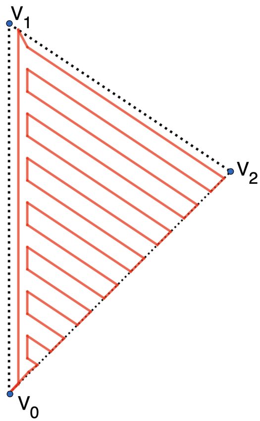
Sustainability 2020, 12, 8878                                                                        3 of 25

regions, and drones with arbitrary flight and range characteristics: however, to demonstrate feasibility
we employ a scenario that is appropriate for applications in developing countries, in which low-cost
drones are used and the area under surveillance contains irregular terrain such that only a limited
number of locations are suitable for charging station installation.
     The rest of the paper is organized as follows: Section 2 presents the material and methods and
presents the assumptions as well as mathematical and computational details of the algorithm used to
solve the problem. Section 3 presents the results, followed by discussion in Section 4. This paper ends
with a conclusion and several ideas for future works.

2. Materials and Methods

2.1. Model Assumptions
      Our CPP algorithm generates a drone mission path under the following assumptions:
•     It is assumed that minimizing the cost of the system is considered to be more important than all
      other factors. This will usually be the case in resource-poor situations. However, if the user wants
      to investigate alternative system configurations that give shorter mission times, (s)he may reduce
      the CS radius parameter (explained below), which will lead to higher-cost systems with reduced
      mission times.
•     The area that is to be surveilled (henceforth referred to as “the field”) is polygonal and may thus
      be completely specified by the vertices of the bounding polygon.
•     The drone is assumed to have a single flight mode, in which the drone’s camera runs continuously
      and video information is either stored onboard or is continuously transmitted back as the
      drone flies.
•     The drone’s height, velocity, and power consumption are assumed to be constant throughout the
      drone’s mission (except when recharging).
•     A start location is specified by the user, which is a point (presumably somewhere on the field’s
      edge) from which the drone is originally launched to conduct its mission. When launched from
      the start location, the drone is fully charged.
•     Possible CS locations are scattered throughout the region and are specified to the algorithm by
      the user. This assumption is included to accommodate the situation where some locations within
      the field are more favorable than others for CS installation. If all locations are equally favorable,
      the user can input a regular or quasirandom lattice of points that fills the entire region.

2.2. Mission Path Planning Algorithm Justification and Outline
      In developing a cost- and time-minimizing mission path, we first take into account the limited
range of drones, which imposes hard constraints on the set of charging stations. In particular,
every point in the field must be reachable by a drone that originates its flight from a charging station
and subsequently returns to a charging station. In our algorithm, we impose the condition that for
every field point there is at least one charging station from which a round trip can be made to that
particular field point. Since minimizing the number of CSs is our primary goal, we restrict possible
solutions to those sets of CSs that both satisfy the constraint and have minimal size.
      Given these possible CS solutions, our goal is to select a solution that minimizes mission time.
It would be much too computationally intensive to compute mission times for a large number of
possible solutions. Instead, we select a set of CSs that minimizes the maximum distance from field point
to nearest charging station, where the maximum is taken over all points within the field. This criterion
is motivated by the fact that field points that are far from the nearest charging station tend to produce
coverage inefficiency, because reaching them requires flying multiple flyovers of closer field points
(this point is explained in more detail in Section 2.9).
      Once the CS have been decided based on the above criteria, the next step is to design an efficient
path that takes full advantage of the characteristics that have been used to select the CS solution.
Sustainability 2020, 12, 8878                                                                        4 of 25

As noted above, field points that are reached from a far-away CS are likely to have inefficient paths.
For this reason, we assign each field point to nearest charging station. This divides the field into
Voronoi regions. Our strategy is to completely cover each Voronoi region before passing on to the next.
It follows that we need a spanning walk that begins and ends at the starting location.
      Finally, the drone’s path for covering each Voronoi region must be specified. Our construction
is based on the observation that the shortest covering path for a drone with infinite range is a
“boustrophedon” or “lawn-mower” pattern, which provides single coverage throughout the field.
Although a finite-range drone cannot execute a boustrophedon, nonetheless a similar pattern of
nonoverlapping parallel segments can be constructed to obtain a solution that closely resembles a
boustrophedon path, and is nearly as efficient. Our algorithm has a recursive structure, based on the
self-similarity of boustrophedon paths within polygons.
      The steps in the drone path planning algorithm may be summarized as follows:

1.     Initialization of parameters for field specifications, potential CS locations and drone
       range specifications;
2.     Create binary grid representation of the field;
3.     Use iterative linear programming to find a minimal set of CSs that minimizes the maximum
       distance from field points to the nearest CS;
4.     Decompose field into Voronoi cells based on selected CS locations;
5.     Compute a closed spanning walk visiting all CSs using a modified traveling salesman algorithm;
6.     Perform a triangular decomposition of each Voronoi cell;
7.     Construct drone paths within each triangular region.

     In the following subsections, we will describe in more detail the steps listed above. The entire
algorithm was coded in Python, using several pre-existing libraries (as described below). The code is
available on Github (https://github.com/LuisEVT/Optimal_Drone_Field_Coverage).

2.3. Initialization
      In order to use the system, the following parameters must be supplied by the user:

•     Field of view (FOV) radius: The camera’s field of view is assumed to be circular with fixed radius.
      As the drone flies, it takes continuous video pictures, thus covering a strip whose width is twice
      the FOV radius.
•     Drone range: This is the maximum distance that a drone can reliably travel on a full charge.
•     CS radius: The CS radius is the maximum distance between any point in the field and the
      nearest CS. In other words, a CS located at point C services a region that lies within a circle whose
      radius is equal to the CS radius with center at C. The CS radius must necessarily be less than or
      equal to half the drone’s range. However, the user has the option of choosing a smaller CS radius.
      A smaller CS radius will tend to produce solutions that have more CS and shorter surveillance
      mission times.
•     Mesh step: For the sake of numerical computations, the coverage region is represented as a
      rectangular grid, whose mesh size is given by the mesh step.
•     Field vertices: The user specifies the polygonal field area by specifying the field vertices in
      consecutive order. In our simulations we employed three basic shapes (rectangle, square,
      and hexagon, as shown in Figure 1), and each shape had three different sizes corresponding
      to total areas 25, 50, and 100 km2 .
•     Start location: This is the drone launching point, as explained in Section 2.1.
•     CS vector length: according to our assumptions, there will be a number of favorable
      locations within the field for placing the CSs. In our simulation, these favorable locations are
      chosen randomly. The CS vector length gives the number of randomly-generated favorable
Sustainability 2020, 12, 8878 5 of 25
locations within the field. In our simulation, we chose the CS vector length so that there was
an average of 1 favorable location per square kilometer. In practice, the user would determine
favorable locations by observation and supply these locations to the algorithm.
Figure 1. Field shapes used in simulations, with vertices marked. Vertices ( x1 , y1 ) are placed at the
start location, which has coordinates (0, 0).
Table 1 summarizes the values of these parameters that were used in the simulations in this paper,
along with symbols used to represent them in our subsequent description of the algorithm.
Table 1. Table of user-supplied parameters.
Name Symbol Value(s) in Simulation
FOV radius ρ 0.025 km
Drone range d 8 km
Drone velocity v 25 km/h
CS radius R 2.0, 2.5, 3.0, 3.5, 3.9 km
Mesh step s 0.02 km
Field vertices ( xn , yn ) Various (see Figure 1)
Field area A 25, 50, 100
Start location (ι x , ι y ) (0, 0)
CS vector length δ 25, 50, 100
2.4. Coverage Field Specification
Next, x and y mesh grid matrices are generated to discretize a rectangular region containing
the field. The x values run from xmin ≡ minn xn to xmax ≡ maxn xn and the y values run from
ymin ≡ minn yn to ymax ≡ maxn yn , both with the same mesh step s. These x and y values are used
to create a list of ( x, y) points within the rectangle, of which some are in the field and some are not,
as shown in Figure 2a. The points in this list that lie in the field are extracted by inputting the field
vertices into the Path class and using the contains_points() function from the matplotlib.path
package in Python. The list of points that lie within the field is further reduced by removing points
that are within a distance R of the start location (ι x , ι y ): these points are removed because they can be
reached from the start location and will not need another charging station to cover them. The remaining
list of ( x, y) points form a grid that discretizes the field area that needs to be covered using charging
stations, as shown in Figure 2b.Sustainability 2020, 12, 8878 6 of 25
(a) (b)
Figure 2. (a) Points in the discretized rectangular (x,y) meshgrid that includes field points, for a
pentagonal field.The outline of the field is shown as a dashed line. (b) Remaining grid points within
the field after applying contain_points() and removing points within R of the start location (0,0).
2.5. Charging Station Location Selection
The primary optimization parameter is the number of CSs, because minimizing the number of
CSs minimizes the cost of the system. The optimal solution must also ensure that each grid point
within the field is within a distance R of the nearest CS. We may formulate the minimization problem
as a linear program as follows:
Minimize ~1 T~z subject to A~z ≥ ~1 with zk ∈ {0, 1} (1)
where:
• K and M are the number of candidate CS and the number of points in the field discretization,
respectively.
• ~1 is a K × 1 vector of all 1’s.
• A is a M × K incidence matrix. The entry Amk is equal to 1 if the mth grid point in the field
discretization is within a distance R of CS k, and 0 otherwise.
• ~z is a K × 1 solution vector. Interpreted as a logical index vector: zk = 1 if CS k is in the solution,
and zk = 0 otherwise.
In (1), the scalar quantity ~1 T~z represents the total number of CS in the solution, which is the quantity
to be minimized. The condition A~z ≥ ~1 represents M inequalities that guarantee that each of the M
grid points within the field lies within a distance R of at least one CS.
Our code uses the glpk.ilp integer linear program solver from the cvxopt convex optimization
package. This solver implements the branch-and-bound algorithm. As mentioned in Section 2.2,
the value of R is successively reduced from its initial value until either the number of CSs in the
solution increases or no solution exists.
2.6. Creation of Voronoi Regions
Once we have selected a particular set of CS locations, the next step is to design the drone’s path.
The first step in this process is to identify the ( x, y) locations belonging to the jth charging station:
that is, the points in the field which are reached following a recharge at station j.
Any finite set of J points Pj , j = 1 . . . J in the ( x, y) plane determines a set of J Voronoi cells,
where each Voronoi cell is a convex polygon that contains exactly one of the points (see Figure 3a).
The Voronoi cell for point Pj consists of all points in the plane that are closer to point Pj than any of the
J − 1 other points. Thus the Voronoi cell of each CS corresponds to the region which is closest to that
CS from among all CS. If we intersect the j’th Voronoi cell with the field, the result gives the region to
be covered by means of drone trips between which the drone is recharged at CS j.Sustainability 2020, 12, 8878 7 of 25
The Python package spatial in the library SciPy (version 1.4.1) contains the class Voronoi which
return vertices of Voronoi cells, when the point ( x, y) locations are supplied as inputs. The class only
returns vertices of finite regions (see Figure 3a): thus, an additional four proxy sites located outside of
the field were used to ensure that all Voronoi cells of interest were finite. The four proxy sites formed
a rectangle that contained the entire field, as shown in Figure 3b. Once these finite Voronoi regions
were generated, the field boundaries were used to restrict the Voronoi regions so that the resulting
cells were all contained within the field. For this purpose, the Python library Shapely was used to
determine the polygons obtained by intersecting the polygonal Voronoi regions with the user-specified
field polygon, as shown in Figure 3c.
(a) Unbounded Voronoi regions (b) Bounded Voronoi regions
(c) Final Voronoi regions
Figure 3. Calculation of Voronoi regions inside a pentagonal field. (a) Unbounded Voronoi regions
for 5 CS. These are not returned by the Python class Voronoi. (b) Bounded Voronoi regions resulting
when four proxy points (indicated as hollow dots) are added. The boundary of the pentagonal field is
represented as a dotted line. (c) Final Voronoi regions obtained by intersecting Voronoi polygons with
the pentagonal field.
2.7. Charging Station Spanning Walk Construction
Once the locations of the CSs have been fixed, the next step is to specify the actual drone mission
path. To cover the entire region, the drone will have to pass from Voronoi region to Voronoi region
and cover each visited region by repeated trips to the region’s CS. In order to characterize the drone’s
motion from CS to CS, we recast the situation in graph theoretic terms. Each CS is identified as a vertex
in a graph, and two vertices are joined by an edge if the Voronoi regions of the two corresponding
CSs share a common bounding edge. This path linking the different CSs may be described in graph
theoretic terms as a closed spanning walk: that is, a sequence of vertices joined by edges that contains
all vertices in the graph, such that the first and last vertex is the same. Note that according to this
definition, both vertices and edges can be repeated in the walk: repetition may in fact be necessary to
attain the spanning property, as shown in Figure 4a. In our construction of the closed spanning walk,
we shall minimize the total number of edges, because extra edges may lead to duplicate coverage.
In order to pose the closed spanning walk construction as a linear programming problem,
we associate the walk with a Hamiltonian cycle in a larger graph as follows. With the given vertices,
we create a complete weighted graph such that between every two vertices there is an edge. The edge
between two vertices is assigned a weight equal to the number of edges in the shortest path within theSustainability 2020, 12, 8878 8 of 25
original graph joining the two vertices. A closed spanning walk in the original graph that minimizes
edges corresponds to a Hamiltonian cycle in the new graph which minimizes the sum of edge
weights. Finding a weight-minimizing Hamiltonian cycle is equivalent to the classical traveling
salesman problem. The steps of the algorithm for finding the closed spanning walk that visits each CS
are summarized as follows:
(a) Create a 0–1 vertex-vertex adjacency matrix, where vertices represent CSs and adjacent vertices
represent CSs with adjacent Voronoi cells.
(b) Use Dijkstra’s algorithm to find the shortest path linking every pair of vertices in the graph
described by this adjacency matrix.
(c) Create a weight matrix for the complete graph using the weights computed in (b).
(d) Solve for a weight-minimizing Hamiltonian cycle that includes all CSs.
(e) Replace the edges in solution (d) with weights greater than 1 with the intermediate edges obtained
by Dijkstra’s algorithm to obtain the complete walk on the original graph.
(a) CS adjacency graph
(b) Complete weighted graph
Figure 4. (a) Example of a CS adjacency graph. Each vertex represents a CS, and edges are drawn
between CSs whose Voronoi regions share a common edge. Note that in order to form a closed spanning
walk, vertex v2 and edge v1 v2 must be repeated. (b) Complete weighted graph formed from the CS
adjacency graph in (a). Edge weights correspond to the minimum number of edges in a connecting
path between vertices in the original graph.
In our system, for step (b) we made use of the implementation of Dijkstra’s algorithm in the scipy
class scipy.sparse.csgraph. The weight-minimizing Hamiltonian cycle in (d) was found using the
following linear program:
~ T~e subject to M~e = ~2,
Minimize w where ek ∈ {0, 1} (2)
where:
• E and N denote the number of vertices and edges in the graph, respectively;
• ~ is an E × 1 vector , where w j is the weight associated with the j’th edge in the complete graph;
w
• M is a N × E vertex-edge incidence matrix. The entry mij is equal to 1 if node i is an endpoint of
edge j;
• ~2 is an E × 1 matrix of all 2’s.
• ~e is an E × 1 solution vector, interpreted as a logical index vector: e j = 1 if edge j is in the solution,
and e j = 0 otherwise.
The scalar quantity w ~ T~e gives the sum of weights of edges in the Hamiltonian cycle in the complete
graph, which is equal to the number of edges in the corresponding closed spanning walk in the original
graph. The condition M~e ≥ ~2 represents the fact that each vertex in the cycle must have an entering and
leaving edge. When a solution to (2) is computed, the corresponding tour is checked for connectivity.
If the cycle is not connected, then an additional constraint is added to the linear program that preventsSustainability 2020, 12, 8878 9 of 25
this solution—and this process is iterated until an optimal connected cycle is contained. The minimum
connecting paths found using Dijkstra’s algorithm are then used to construct the closed spanning walk
on the original graph.
In the actual drone path, the drone does not fly directly from one CS to another but rather passes
by way of a vertex that is shared by the coverage cells of the two CSs (see Figure 5). There are two
reasons for this. First, the paths between adjacent CSs cover vertices that are far from any CS, when they
do not need to be covered by long round trips to-from a single CS. Second, the straight segments
of the paths between CSs lie along the edges of triangles used in the triangulations of the Voronoi
regions described in the next section, so that the segments are not double-covered when the triangle
interiors are covered as described below. This serves to improve the algorithm’s efficiency in terms of
reducing total mission time. The algorithm is configured so that no segment of the path linking the
CSs is traveled twice in a complete path traversal, as may be seen in Figure 5.
Figure 5. Closed spanning walk linking CS locations (blue line) within a pentagonal-shaped field.
CSs are shown in red, while Voronoi regions are outlined in black. Note that drone does not fly directly
from CS to CS but rather travels by way of common vertices between Voronoi regions as described in
the text.
2.8. Drone Trajectories within Individual Voronoi Cells
To simplify the drone’s coverage of Voronoi cells, the cells were further divided into triangles,
as shown in Figure 6. Suppose that the vertices of the j’th Voronoi region are given by
( p1 , q1 ), . . . , ( pn j , qn j ). Then the region is divided into n j triangles, where the vertices of the i’th
triangle are given by {(u j , v j ), ( pi , qi ), ( pi+1 , qi+1 )}, i = 1, . . . n j (in this expression ( pn j +1 , qn j +1 ) is
identical to ( p1 , q1 )).
The algorithm for finding the drone path within each triangle was programmed as a subroutine.
Before calling the subroutine for a given triangle, the triangle is rotated so that the longest side is
parallel to the y axis and the bottom vertex of the longest side is translated to (0, 0), as shown in
Figure 7. If possible, this vertex is chosen as the CS location, and if necessary, the triangle is reflected
so that all points in the triangle lie in the first quadrant. The linear transformation applied to ( x, y)
may be expressed as: " #! " #" #
x ± cos θ ∓ sin θ x − x0
Q = , (3)
y sin θ cos θ y − y0Sustainability 2020, 12, 8878 10 of 25
where ( x0 , y0 ) is the vertex that is translated to (0, 0); ( x1 , y1 ) is the other vertex of the longest side;
x1 − x0 y1 − y0
sin θ = p ; cos θ = p ;x (4)
( x1 − x0 )2 + ( y1 − y0 )2 ( x1 − x0 )2 + ( y1 − y0 )2
and the ± corresponds to whether the triangle is or is not flipped (− or + respectively).
Figure 6. Triangulation of Voronoi regions for the field configuration shown in Figure 5.
The drone path algorithm used within the triangle is based on a “boustrophedon” (or “lawn
mower”) pattern. Some double coverage is necessary, when multiple recharges are required for the
drone to cover the entire triangle. The drone path that is constructed within the triangle consists of
segments parallel to one the three sides, joined (if necessary) by short connecting segments. The path
is constructed segment by segment, and each time a segment is constructed the remaining region to be
covered remains triangular in shape but with reduced area.
Figure 7. Transformed triangle used as input to the triangle covering path algorithm.
The basic idea of the algorithm is as follows. Let V0 , V1 , V2 be the vertices of the triangle, where V0
is the vertex in which the CS is located, V1 is the farthest vertex from CS, and V2 is the remaining vertex.
The algorithm will always start by traveling from V0 to V1 . Ideally, we want the drone to cover the area
farthest away from the CS to minimize double coverage. One flight path that would accomplish this is:Sustainability 2020, 12, 8878 11 of 25
• V0 to V1 ;
• V1 to V2 ;
• Go back and forth parallel to V1 V2 until the entire region is covered.
This path is shown in Figure 8. However, the fact that the drone has limited range means that,
in practice, the drone will have to break off from this pattern and return to the CS to recharge.
After recharging, the algorithm will restart by having the drone travel to V0 , as seen in Figure 9.
As can seen in the figure, after each drone path segment, the remaining uncovered triangle is similar
to the original triangle but successively smaller and smaller. Consequently, we can reapply the same
algorithm to each smaller triangle to obtain a path that covers the entire original triangle. A flowchart
for the algorithm used to generate path segments in shown in Figure 10. Pseudocodes for the algorithm
and its subfunctions are shown in the appendix. Once the path is completed on a the transformed
triangle, we apply the inverse transformation to obtain the actual path.
Figure 8. Coverage path for drone with unlimited energy.
Figure 9. Drone path within a single triangle automatically generated by the algorithm. Different colors
represent individual drone trajectories between charges. CS is located at (0, 0).Sustainability 2020, 12, 8878 12 of 25
curPoint, maxEnergy,
path = [],
remainEnergy, Start
fPath = []
nxtLoc, CS, V0 , V1 , V2
is curPoint yes Recharge
equal to CS Drone
Return []
no no
Compute
V ef , V 0 , V 0
ei , V
i f
Compute Compute Remaining
Vi = first element in Compute
remaining ef , V 0 , V 0 Energy >
nxtLoc, nxtLoc = (Vi , V0 ) V
ei , V
i f required energy
energy Req Energy
yes
yes
Remaining
is fPath Store V
ei , V
ef , CS
Energy >
empty
no
Req. Energy no in path
yes
Store V
ei , V
ef is Triangle
Return combine(path,fPath)
in path yes covered?
store CS
in path
no
is Triangle
covered? yes
fPath = nextPath()
no
curPoint = V
ef
compute
nxtLoc
Compute
remaining
energy
Relocate
fPath = nextPath()
V0 , V1 , V2
Figure 10. Flowchart for recursive function nextPath().
We illustrate the algorithm process in more detail by showing the construction of the initial path
segment. We consider the case where the CS location (denoted by V0 ) is located at (0, 0) as shown in
(see Figure 7). In this case, the initial segment is parallel to V0 V1 at a perpendicular distance ρ, as shown
in Figure 11. The endpoints of this initial segment are denoted by V e0 ≡ ( xe0 , ye0 ) and V
e1 ≡ ( xe1 , ye1 ),
as shown in the figure. Note that the point V e1 is on the segment V1 V2 . The mathematical expressions
for V
e0 and Ve1 are:
ρ ρ
V0 = x0 + ρ, y0 +
e ; V1 = x1 + ρ, y1 −
e (5)
tan(α) tan( β)
Since we are beginning at V1 , we must also include the short segment from V1 to V
e1 in the path.Sustainability 2020, 12, 8878 13 of 25
Figure 11. Illustration of where V f1 , V 0 , V 0 are located within the triangle when moving parallel
f0 , V
0 1
of V0 V1 .
Once the segment from V e0 to V
e2 is completed, then the remaining uncovered area is a smaller
triangle with vertices {V0 , V1 , V2 } where V00 and V10 are given by:
0 0
2ρ 2ρ
V00 = x0 + 2ρ, y0 + ; V10 = x1 + 2ρ, y1 − , (6)
tan(α) tan( β)
as shown in Figure 11.
At this point, the algorithm has a choice. If there is still enough remaining energy, the drone will
pass from Ve1 to V e 0 , where
e2 by way of point V
1
e10 = ρ sin(α) cos(α)
V xe10 , ye10 − ; e2 =
V x2 − ρ · , y2 − ρ · . (7)
sin( β) sin(γ) sin(γ)
Consequently, the remaining uncovered area is another smaller triangle with vertices {V00 , V100 , V20 }
where V100 and V20 are given by:
2ρ sin(α) cos(α)
V100 = xe10 , ye10 − ; V20 = x2 − 2ρ · , y2 − 2ρ · . (8)
sin( β) sin(γ) sin(γ)
On the other hand, if there is not enough energy, the drone will return from V10 to V00 along a path
that is parallel to V00 V10 at a distance ρ. The equations for this return segment are similar to Equation (6)
except that x1 , y1 , x2 , y2 are replaced by xe1 , ye1 , xe2 , ye2 respectively.
In case the drone does travel to V20 , the drone once again has two options: either return to recharge
or travel back towards V10 . Let us suppose the drone needs to recharge: then it will travel parallel to
V00 V20 , and then return to the CS at V0 to recharge. The mathematical expression for V e 0 and V
e 0 are:
2 0
e20 = sin( β) 0 cos( β) ρ
V x20 − ρ · , y +ρ· e00 =
V x00 , y00 + (9)
sin(γ) 2 sin(γ) sin(α)
The remaining uncovered area is another smaller triangle with vertices {V000 , V100 , V200 } where V000
and V200 are given by:
sin( β) 0 cos( β) 2ρ
V200 = x20 − 2ρ · , y + 2ρ · V000 = x00 , y00 + (10)
sin(γ) 2 sin(γ) sin(α)Sustainability 2020, 12, 8878 14 of 25
After the drone is recharged, the algorithm will start again by sending the drone to V000 and
beginning its journey to cover the remaining area of the triangle. Figure 12 shows the final drone path
produced by the system for the field configuration shown in Figures 5 and 6.
Figure 12. Completed drone path for entire pentagonal-shaped field, with CS radius = 2.5 km. The red
dots denote CS locations, while the blue lines show the Voronoi cells. The different colored lines
indicate flights made on a single charge. The spanning walk identified in Figure 5 shows as white lines.
2.9. Performance Evaluation
The two performance parameters of practical interested are the number of CSs and the total
mission time. The efficiency of the algorithm with respect to these two parameters was measured
as follows.
It is known that the most efficient cover of a plane by circles is obtained by a circumscribing the
hexagons in a “honeycomb” lattice [54]. This implies that regular hexagonal-shaped cells cover the
maximum area with the fewest possible cells, given the cells’ radius is constrained to be less than R.
To measure the CS efficiency for a configuration with CS coverage radius R, we divided the mean area
per Voronoi cell by the area of a hexagon with radius R. This gives a dimensionless measure that can
be compared across different field sizes and shapes.
As far as mission time, mission time may be broken up into (travel time ) + (recharge time).
The travel time was computed as (travel distance) / cruise velocity. The recharge time is computed as
(travel time) × (power consumption) / recharge power. It follows that the tour time is equal to:
cruise velocity + power consumption
Tour time = (Tour distance) . (11)
(cruise velocity)(recharge power)
Equation (11) shows that tour time is proportional to tour distance. It follows that minimizing
tour time is equivalent to minimizing tour distance.
We have mentioned in Section 2.2 that a maximally efficient boustrophedon path that passes
over all field points exactly once is not possible for drones of limited range. Instead, a drone may
need to travel multiple times over the same area, consequently increasing the total travel distance.Sustainability 2020, 12, 8878 15 of 25
We may derive a lower bound on the total travel distance for a complete surveillance mission using
the following notations:
• D (r ) is the total distance that the drone flies while its distance to the nearest CS is greater than r,
for 0 ≤ r ≤ R. Note that D ( R) = 0, while D (0) is equal to the total distance that the drone flies
during its surveillance mission (denoted by D).
• A(r ) is the field area that lies farther than a distance r of the nearest CS, for 0 ≤ r ≤ R. Note that
A( R) = 0, while A(0) is the total field area (denoted by A).
Then we have:
2r
D − D (r ) ≥ D, 0 ≤ r ≤ R. (12)
d
The inequality in (12) expresses the fact that on each single charge, the drone can fly a total distance at
most d of which at least 2r is within radius r. We also have:
2ρ · D (r ) ≥ A(r ), 0 ≤ r ≤ R. (13)
In (13) the left-hand side represents the total area which the drone camera’s FOV passes over while
flying farther than r from the nearest CS, which must be greater than or equal to the total field area
that is farther than r from the nearest CS. Combining (12) and (13) gives:
A(r )
d
D≥ · max . (14)
2ρ r d − 2r
A dimensionless and scalable measure of efficiency was obtained by taking the theoretical
minimum mission distance derived in (14) and dividing by the achieved mission distance. In this way,
a mission efficiency of 1 represents the shortest possible mission for the given CS configuration.
2.10. Simulation Specifications
In order to evaluate the effectiveness of the algorithm, we applied it to a variety of scenarios.
Parameter values used are listed in the last column of Table 1. These parameters were chosen to
match the specifications of the Mavic Air drone with 2375 mAh battery [55], together with the Heisha
C300 solar-powered charging pad [56]. Three different field shapes (3:1 rectangle, square, octagon)
were used, as well as three different total areas (25, 50, 100 km2 ). For each of these 9 field configurations,
100 different random CS configurations were generated, and run for 5 different initial CS coverage radii,
as given in Table 1. Smaller initial radii led to solutions with more CSs and shorter mission times.
All simulations were done on a MacBook Pro with a single 8-core 2.3 GHz Intel Core i9
processor and 16 GB RAM, running Python 3.7.6 with a Spyder 4.0.1 interface. Figure 13 shows
the runtimes achieved, where each single run of the algorithm is shown as a dot on the graph.
Runtimes were under 100 s, even for the largest configuration, demonstrating the algorithm’s practical
applicability even for large scenarios.Sustainability 2020, 12, 8878 16 of 25
Figure 13. Algorithm runtimes for all simulation runs.
3. Results
Results are graphically summarized in Figures 14 and 15, while Table A1 gives numerical statistics.
In calculating the coverage time, the cruise speed was taken as 25 km and a charge time: flight time
ratio of 2:1 was used.
The first row of graphs in Figure 14 shows the expected field per CS. For fields of size 25 km2 ,
we may expect to use 1 CS for every 4 km2 when the CS radius is 2 and about 1 CS for every 11 km2
when the CS radius is 4. For larger areas, a much greater efficiency can be achieved; 1 CS for every
6 km2 when the CS radius is 2 and about 1 CS for every 20 km2 when the CS radius is 3.9. This implies
that only about 1/3 as many CSs would be required if the larger CS radius is used for the design.
The second row of graphs in Figure 14 measures the CS efficiencies, which ranged from about
35% to above 70%. Greater efficiencies were observed with more regular fields (square and octagon as
opposed to rectangle), larger fields, and smaller CS coverage radii.
Figure 14. Comparison of algorithm coverage performance for different field configurations and CS
coverage radii. Error bars correspond to the standard deviation computed from 100 runs for each field
size/shape/CS radius configuration.
Mission times per field area are shown in the first row of graphs in Figure 15. The similarity
between the graphs for different field sizes shows that mission times are roughly proportional toSustainability 2020, 12, 8878 17 of 25
total field area. For small areas the coverage radius had little effect on the total mission time, but for
the largest area size total mission times were up to 40% larger for CS coverage radius equal to 4 km
compared to CS coverage radius equal to 2 km. Mission efficiencies ranged from about 70% to
about 90%. Greater efficiencies were observed with smaller field sizes and smaller CS coverage radii.
For the smallest field size, the efficiency was roughly independent of the CS coverage radius.
The information in Figures 14 and 15 is combined in Figure 16 to produce Pareto frontiers
showing the tradeoff between mission time and number of charging stations. Information for all of
the individual runs is plotted. There is considerable variation in the mission time per area for a given
value of covered area per CS, especially for larger coverage areas. The similarity between the three
graphs shows that the tradeoff is relatively independent of the field size.
Figure 15. Comparison of algorithm mission time performance for different field configurations and
CS coverage radii. Error bars correspond to the standard deviation computed from 100 runs for each
field size/shape/CS radius configuration.
Figure 16. Pareto frontiers showing the tradeoff between minimizing mission time per area and
maximizing covered area per charging station.Sustainability 2020, 12, 8878 18 of 25
4. Discussion
The results observed are reasonable from a geometric point of view. For smaller field sizes and
large CS coverage radii, it is unavoidable that a large portion of the CS coverage region will lie outside
of the field. This is why lower CS efficiencies were observed in Figure 14 for the 25 km2 field sizes.
As the size increases, a smaller proportion of Voronoi cells is near the field boundary, so the wasted
area is less. For large cells, the increased CS efficiency comes at the cost or lower mission efficiency.
This is because greater CS efficiency means larger cells, which implies more area that is far from the
nearest CS which will require repeated trips that cover the same area multiple times.
5. Conclusions
We have developed a software system that generates a comprehensive drone surveillance plan
for large, inaccessible agricultural or forested areas. Our results indicate feasible numbers of CSs
and mission times for a variety of field shapes and sizes. We have demonstrated the adaptability of
the software. Future possibilities for research include introducing more realistic conditions such as
variable winds, drone’s multiple operating modes, etc.
Author Contributions: Conceptualization, A.F., J.L.K.E.F., and C.T.; methodology, C.T., L.V.T., and S.-K.T.;
software, L.V.T. and S.-K.T.; validation, L.V.T. and C.T.; formal analysis, L.V.T. and C.T.; writing—original draft
preparation, L.V.T.; writing—review and editing, J.L.K.E.F., C.T., and A.F.; supervision, A.F. and C.T. All authors
have read and agreed to the published version of the manuscript.
Funding: This research received no external funding.
Conflicts of Interest: The authors declare no conflict of interest.Sustainability 2020, 12, 8878 19 of 25
Appendix A. Data Tables
Table A1. Data summary for each configuration.
Shape Area CS Radius nCS Total Distance Travel Theoretical Best Distance Total Mission Time Theo. Best Mission Time
- - - Mean std Mean std Mean std Mean std Mean std
Octagon 25 2.0 5.60 0.49 577.68 3.15 514.03 1.52 69.32 0.38 61.68 0.18
Octagon 25 2.5 4.03 0.17 585.30 5.17 520.83 1.75 70.24 0.62 62.50 0.21
Octagon 25 3.0 2.97 0.17 604.50 15.88 531.42 4.85 72.54 1.91 63.77 0.58
Octagon 25 3.5 2.27 0.45 664.41 42.99 549.09 11.59 79.73 5.16 65.89 1.39
Octagon 25 3.9 2.01 0.10 696.21 31.01 555.98 3.03 83.54 3.72 66.72 0.36
Octagon 50 2.0 9.29 0.46 1149.18 5.11 1032.16 1.75 137.90 0.61 123.86 0.21
Octagon 50 2.5 6.36 0.48 1172.33 10.32 1049.87 4.42 140.68 1.24 125.98 0.53
Octagon 50 3.0 5.00 0.00 1223.12 29.13 1066.90 2.77 146.77 3.50 128.03 0.33
Octagon 50 3.5 4.00 0.00 1351.37 55.40 1091.90 6.63 162.16 6.65 131.03 0.80
Octagon 50 3.9 3.09 0.29 1470.21 75.66 1138.25 19.82 176.43 9.08 136.59 2.38
Octagon 100 2.0 16.36 0.63 2299.21 6.25 2070.70 2.90 275.91 0.75 248.48 0.35
Octagon 100 2.5 10.50 0.52 2345.68 12.95 2116.30 6.96 281.48 1.55 253.96 0.83
Octagon 100 3.0 7.98 0.20 2520.19 51.55 2165.86 8.36 302.42 6.19 259.90 1.00
Octagon 100 3.5 6.01 0.10 2945.54 74.01 2244.15 14.97 353.46 8.88 269.30 1.80
Octagon 100 3.9 5.02 0.14 3221.37 79.58 2317.22 22.71 386.56 9.55 278.07 2.73
Rectangle 25 2.0 6.14 0.57 574.38 4.09 513.08 1.47 68.93 0.49 61.57 0.18
Rectangle 25 2.5 4.19 0.39 578.60 6.41 520.60 2.10 69.43 0.77 62.47 0.25
Rectangle 25 3.0 3.06 0.24 622.16 18.73 531.62 3.39 74.66 2.25 63.79 0.41
Rectangle 25 3.5 3.00 0.00 625.99 17.08 532.38 2.22 75.12 2.05 63.89 0.27
Rectangle 25 3.9 2.06 0.24 777.67 41.05 566.75 14.40 93.32 4.93 68.01 1.73
Rectangle 50 2.0 10.07 0.57 1146.14 5.44 1030.17 2.13 137.54 0.65 123.62 0.26
Rectangle 50 2.5 7.11 0.40 1172.43 10.29 1045.41 4.27 140.69 1.23 125.45 0.51
Rectangle 50 3.0 5.08 0.31 1269.67 34.03 1068.52 5.60 152.36 4.08 128.22 0.67
Rectangle 50 3.5 4.04 0.20 1406.68 46.76 1092.11 5.06 168.80 5.61 131.05 0.61
Rectangle 50 3.9 3.67 0.47 1502.07 134.27 1110.79 25.23 180.25 16.11 133.30 3.03
Rectangle 100 2.0 17.46 0.61 2295.22 6.94 2066.85 2.58 275.43 0.83 248.02 0.31
Rectangle 100 2.5 11.04 0.49 2346.95 14.90 2111.61 6.47 281.63 1.79 253.39 0.78
Rectangle 100 3.0 8.38 0.49 2566.02 66.03 2160.66 12.54 307.92 7.92 259.28 1.51
Rectangle 100 3.5 7.00 0.14 2860.30 66.66 2208.43 13.91 343.24 8.00 265.01 1.67
Rectangle 100 3.9 5.74 0.58 3255.78 172.34 2274.21 42.62 390.69 20.68 272.91 5.11
Square 25 2.0 5.69 0.53 574.32 3.44 514.23 1.58 68.92 0.41 61.71 0.19
Square 25 2.5 4.02 0.14 579.08 5.14 521.85 1.45 69.49 0.62 62.62 0.17
Square 25 3.0 3.22 0.42 621.40 24.66 530.81 5.86 74.57 2.96 63.70 0.70
Square 25 3.5 3.00 0.00 634.01 12.22 533.77 3.98 76.08 1.47 64.05 0.48
Square 25 3.9 2.28 0.45 718.45 53.28 555.34 13.43 86.21 6.39 66.64 1.61
Square 50 2.0 9.43 0.50 1146.63 5.22 1032.23 2.11 137.60 0.63 123.87 0.25
Square 50 2.5 6.51 0.50 1170.59 12.08 1049.77 4.80 140.47 1.45 125.97 0.58
Square 50 3.0 4.79 0.41 1244.96 34.02 1073.87 10.17 149.39 4.08 128.86 1.22
Square 50 3.5 4.00 0.00 1323.30 40.51 1095.39 5.76 158.80 4.86 131.45 0.69
Square 50 3.9 3.97 0.17 1336.64 82.51 1097.30 12.05 160.40 9.90 131.68 1.45
Square 100 2.0 16.80 0.70 2295.17 6.83 2069.55 3.05 275.42 0.82 248.35 0.37
Square 100 2.5 10.91 0.43 2351.34 15.09 2113.64 5.74 282.16 1.81 253.64 0.69
Square 100 3.0 8.02 0.14 2547.13 52.99 2167.99 9.08 305.66 6.36 260.16 1.09
Square 100 3.5 6.11 0.31 3020.36 98.30 2244.43 20.44 362.44 11.80 269.33 2.45
Square 100 3.9 5.04 0.20 3354.20 101.54 2323.74 21.50 402.50 12.18 278.85 2.58Sustainability 2020, 12, 8878 20 of 25
Appendix B. Algorithms
Algorithm A1: Triangular drone path algorithm.
Function nextPath(curPoint, maxEnergy, remainEnergy, nxtLoc, CS, V0 , V1 , V2 ):
/* Return a list of coordinates */
path = [];
fPath = [];
if curPoint == CS then
remainEnergy = maxEnergy;
end
V
ei , Vef = computeVei V
ef (nxtLoc);
Vi0 , Vf0 = computeVi0 , Vf0 (nxtLoc);
reqEnergy = Energy from curPoint to V ei to V
ef ;
if remainEnergy ≥ reqEnergy then
pathSustainability 2020, 12, 8878 21 of 25
Algorithm A2: Help Functions 1
Function computeVei V
ef (nxtLoc):
/* Return the segment parallel to Vi and Vf by distance ρ */
if nxtLoc = (V0 , V1 ) then
return Ve0 , V
e1
end
else if nxtLoc = (V0 , V1 ) then
return Ve0 , V
e1
end
else if nxtLoc = (V2 , V1 ) then
return Ve2 , V
e1
end
else if nxtLoc = (V2 , V0 ) then
return Ve2 , V
e0
end
else if nxtLoc = (V1 , V0 ) then
return Ve1 , V
e0
end
Function computeVi0 Vf0 (nxtLoc):
/* Return the segment parallel to Vi and Vf by distance 2ρ */
if nxtLoc = (V0 , V1 ) then
return V00 , V10
end
else if nxtLoc = (V1 , V2 ) then
return V00 , V10
end
else if nxtLoc = (V2 , V1 ) then
return V20 , V10
end
else if nxtLoc = (V2 , V0 ) then
return V20 , V00
end
else if nxtLoc = (V1 , V0 ) then
return V10 , V00
endSustainability 2020, 12, 8878 22 of 25
Algorithm A3: Help Functions 2
Function computeV1 V2 V3 (nxtLoc, Vi0 , Vf0 ):
/* Return V0 , V1 , V2 */
if nxtLoc = (V0 , V1 ) then
return Vi0 , Vf0 , V2
end
else if nxtLoc = (V1 , V2 ) then
return V0 , Vi0 , Vf0
end
else if nxtLoc = (V2 , V1 ) then
return V0 , Vf0 , Vi0
end
else if nxtLoc = (V2 , V0 ) then
return Vf0 , V1 , Vi0
end
else if nxtLoc = (V1 , V0 ) then
return Vf0 , Vi0 , V2
end
Function computeNxtLoc(nxtLoc):
/* RETURN NEXT SEGMENT OF INTEREST */
if nxtLoc = (V0 , V1 ) then
return (V1 , V2 )
end
else if nxtLoc = (V1 , V2 ) then
return (V2 , V1 )
end
else if nxtLoc = (V2 , V1 ) then
return (V1 , V2 )
end
else if nxtLoc = (V2 , V0 ) then
return (V0 , V1 )
end
else if nxtLoc = (V1 , V0 ) then
return (V0 , V1 )
end
References
1. Song, L.J.; Fan, Q. The design and implementation of a video surveillance system for large scale wind farm.
Adv. Mater. Res. Trans. Tech. Publ. 2012, 361, 1257–1262. [CrossRef]
2. Lloret, J.; Garcia, M.; Bri, D.; Sendra, S. A wireless sensor network deployment for rural and forest fire
detection and verification. Sensors 2009, 9, 8722–8747. [CrossRef] [PubMed]
3. Lloret, J.; Bosch, I.; Sendra, S.; Serrano, A. A wireless sensor network for vineyard monitoring that uses
image processing. Sensors 2011, 11, 6165–6196. [CrossRef] [PubMed]
4. Garcia-Sanchez, A.J.; Garcia-Sanchez, F.; Garcia-Haro, J. Wireless sensor network deployment for
integrating video-surveillance and data-monitoring in precision agriculture over distributed crops.
Comput. Electron. Agric. 2011, 75, 288–303. [CrossRef]
5. Garcia-Sanchez, A.J.; Garcia-Sanchez, F.; Losilla, F.; Kulakowski, P.; Garcia-Haro, J.; Rodríguez, A.;
López-Bao, J.V.; Palomares, F. Wireless sensor network deployment for monitoring wildlife passages.
Sensors 2010, 10, 7236–7262. [CrossRef]
6. Eisenbeiss, H. A mini unmanned aerial vehicle (UAV): System overview and image acquisition. Int. Arch.
Photogramm. Remote Sens. Spat. Inf. Sci. 2004, 36, 1–7.
7. Freeman, P.K.; Freeland, R.S. Agricultural UAVs in the US: Potential, policy, and hype. Remote Sens. Appl.
Soc. Environ. 2015, 2, 35–43.Sustainability 2020, 12, 8878 23 of 25
8. Herwitz, S.; Johnson, L.; Dunagan, S.; Higgins, R.; Sullivan, D.; Zheng, J.; Lobitz, B.; Leung, J.; Gallmeyer, B.;
Aoyagi, M.; et al. Imaging from an unmanned aerial vehicle: Agricultural surveillance and decision support.
Comput. Electron. Agric. 2004, 44, 49–61. [CrossRef]
9. Jarman, M.; Vesey, J.; Febvre, P. Unmanned Aerial Vehicles (UAVs) for UK Agriculture: Creating an Invisible
Precision Farming Technology. White Paper, 19 July 2016.
10. Barrero, O.; Perdomo, S.A. RGB and multispectral UAV image fusion for Gramineae weed detection in rice
fields. Precis. Agric. 2018, 19, 809–822. [CrossRef]
11. Hassanein, M.; El-Sheimy, N. An efficient weed detection procedure using low-cost uav imagery system for
precision agriculture applications. Int. Arch. Photogramm. Remote Sens. Spat. Inf. Sci. 2018. [CrossRef]
12. Pallottino, F.; Menesatti, P.; Figorilli, S.; Antonucci, F.; Tomasone, R.; Colantoni, A.; Costa, C. Machine vision
retrofit system for mechanical weed control in precision agriculture applications. Sustainability 2018, 10, 2209.
[CrossRef]
13. Huang, Y.; Reddy, K.N.; Fletcher, R.S.; Pennington, D. UAV low-altitude remote sensing for precision
weed management. Weed Technol. 2018, 32, 2–6. [CrossRef]
14. Shafian, S.; Rajan, N.; Schnell, R.; Bagavathiannan, M.; Valasek, J.; Shi, Y.; Olsenholler, J. Unmanned
aerial systems-based remote sensing for monitoring sorghum growth and development. PLoS ONE
2018, 13, e0196605. [CrossRef] [PubMed]
15. Han, L.; Yang, G.; Yang, H.; Xu, B.; Li, Z.; Yang, X. Clustering field-based maize phenotyping of plant-height
growth and canopy spectral dynamics using a UAV remote-sensing approach. Front. Plant Sci. 2018, 9, 1638.
[CrossRef] [PubMed]
16. Iwasaki, K.; Torita, H.; Abe, T.; Uraike, T.; Touze, M.; Fukuchi, M.; Sato, H.; Iijima, T.; Imaoka, K.; Igawa, H.
Spatial pattern of windbreak effects on maize growth evaluated by an unmanned aerial vehicle in Hokkaido,
northern Japan. Agrofor. Syst. 2019, 93, 1133–1145. [CrossRef]
17. Mahajan, U.; Raj, B. Drones for normalized difference vegetation index (NDVI), to estimate crop health for
precision agriculture: A cheaper alternative for spatial satellite sensors. In Proceedings of the International
Conference on Innovative Research in Agriculture, Food Science, Forestry, Horticulture, Aquaculture,
Animal Sciences, Biodiversity, Ecological Sciences and Climate Change (AFHABEC-2016), Delhi, India,
22 October 2016; Volume 22.
18. Albetis, J.; Jacquin, A.; Goulard, M.; Poilvé, H.; Rousseau, J.; Clenet, H.; Dedieu, G.; Duthoit, S. On the
potentiality of UAV multispectral imagery to detect Flavescence dorée and Grapevine Trunk Diseases.
Remote Sens. 2019, 11, 23. [CrossRef]
19. Kerkech, M.; Hafiane, A.; Canals, R. Deep leaning approach with colorimetric spaces and vegetation indices
for vine diseases detection in UAV images. Comput. Electron. Agric. 2018, 155, 237–243. [CrossRef]
20. Ronchetti, G.; Mayer, A.; Facchi, A.; Ortuani, B.; Sona, G. Crop Row Detection through UAV Surveys to
Optimize On-farm Irrigation Management. Remote Sens. 2020, 12, 1967. [CrossRef]
21. Chen, A.; Orlov-Levin, V.; Meron, M. Applying high-resolution visible-channel aerial imaging of crop
canopy to precision irrigation management. Agric. Water Manag. 2019, 216, 196–205. [CrossRef]
22. Stein, M.; Bargoti, S.; Underwood, J. Image based mango fruit detection, localisation and yield estimation
using multiple view geometry. Sensors 2016, 16, 1915. [CrossRef]
23. Zhou, X.; Zheng, H.; Xu, X.; He, J.; Ge, X.; Yao, X.; Cheng, T.; Zhu, Y.; Cao, W.; Tian, Y. Predicting grain yield
in rice using multi-temporal vegetation indices from UAV-based multispectral and digital imagery. ISPRS J.
Photogramm. Remote Sens. 2017, 130, 246–255. [CrossRef]
24. Yeom, J.; Jung, J.; Chang, A.; Maeda, M.; Landivar, J. Automated open cotton boll detection for yield
estimation using unmanned aircraft vehicle (UAV) data. Remote Sens. 2018, 10, 1895. [CrossRef]
25. Mardanisamani, S.; Maleki, F.; Hosseinzadeh Kassani, S.; Rajapaksa, S.; Duddu, H.; Wang, M.; Shirtliffe, S.;
Ryu, S.; Josuttes, A.; Zhang, T.; et al. Crop lodging prediction from UAV-acquired images of wheat and
canola using a DCNN augmented with handcrafted texture features. In Proceedings of the IEEE Conference
on Computer Vision and Pattern Recognition Workshops 2019, Long Beach, CA, USA, 16–20 June 2019.
26. Zhang, Z.; Flores, P.; Igathinathane, C.; L Naik, D.; Kiran, R.; Ransom, J.K. Wheat Lodging Detection from
UAS Imagery Using Machine Learning Algorithms. Remote Sens. 2020, 12, 1838. [CrossRef]
27. Zhao, X.; Yuan, Y.; Song, M.; Ding, Y.; Lin, F.; Liang, D.; Zhang, D. Use of unmanned aerial vehicle imagery
and deep learning unet to extract rice lodging. Sensors 2019, 19, 3859. [CrossRef]Sustainability 2020, 12, 8878 24 of 25
28. Pádua, L.; Marques, P.; Hruška, J.; Adão, T.; Peres, E.; Morais, R.; Sousa, J.J. Multi-temporal vineyard
monitoring through UAV-based RGB imagery. Remote Sens. 2018, 10, 1907. [CrossRef]
29. De Castro, A.I.; Jimenez-Brenes, F.M.; Torres-Sánchez, J.; Peña, J.M.; Borra-Serrano, I.; López-Granados, F.
3-D characterization of vineyards using a novel UAV imagery-based OBIA procedure for precision
viticulture applications. Remote Sens. 2018, 10, 584. [CrossRef]
30. Tsouros, D.C.; Bibi, S.; Sarigiannidis, P.G. A review on UAV-based applications for precision agriculture.
Information 2019, 10, 349. [CrossRef]
31. Choset, H. Coverage for robotics—A survey of recent results. Ann. Math. Artif. Intell. 2001, 31, 113–126.
[CrossRef]
32. Oksanen, T.; Visala, A. Coverage path planning algorithms for agricultural field machines. J. Field Robot.
2009, 26, 651–668. [CrossRef]
33. Jin, J.; Tang, L. Coverage path planning on three-dimensional terrain for arable farming. J. Field Robot.
2011, 28, 424–440. [CrossRef]
34. Hameed, I.A. Intelligent coverage path planning for agricultural robots and autonomous machines on
three-dimensional terrain. J. Intell. Robot. Syst. 2014, 74, 965–983. [CrossRef]
35. Kakaes, K.; Greenwood, F.; Lippincott, M.; Dosemagen, S.; Meier, P.; Wich, S. Drones and Aerial Observation:
New Technologies for Property Rights. In Human Rights, and Global Development: A Primer; New America:
Washington, DC, USA, 2015; pp. 514–519.
36. Ghaddar, A.; Merei, A. Energy-Aware Grid Based Coverage Path Planning for UAVs. In Proceedings of the
Thirteenth International Conference on Sensor Technologies and Applications SENSORCOMM, Nice, France,
27–31 October 2019; pp. 27–31.
37. Vasquez-Gomez, J.I.; Herrera-Lozada, J.C.; Olguin-Carbajal, M. Coverage path planning for surveying
disjoint areas. In Proceedings of the 2018 International Conference on Unmanned Aircraft Systems (ICUAS),
Dallas, TX, USA, 12–15 June 2018; pp. 899–904.
38. Coombes, M.; Chen, W.H.; Liu, C. Boustrophedon coverage path planning for UAV aerial surveys
in wind. In Proceedings of the 2017 International Conference on Unmanned Aircraft Systems (ICUAS),
Miami, FL, USA, 13–16 June 2017; pp. 1563–1571.
39. Barrientos, A.; Colorado, J.; Cerro, J.D.; Martinez, A.; Rossi, C.; Sanz, D.; Valente, J. Aerial remote sensing
in agriculture: A practical approach to area coverage and path planning for fleets of mini aerial robots.
J. Field Robot. 2011, 28, 667–689. [CrossRef]
40. Almeida, A.; Ramalho, G.; Santana, H.; Tedesco, P.; Menezes, T.; Corruble, V.; Chevaleyre, Y.
Recent advances on multi-agent patrolling. In Brazilian Symposium on Artificial Intelligence; Springer:
Berlin/Heidelberg, Germany, 2004; pp. 474–483.
41. Pasqualetti, F.; Franchi, A.; Bullo, F. On cooperative patrolling: Optimal trajectories, complexity analysis,
and approximation algorithms. IEEE Trans. Robot. 2012, 28, 592–606. [CrossRef]
42. Huang, W.H. Optimal line-sweep-based decompositions for coverage algorithms. In Proceedings of the
2001 ICRA IEEE International Conference on Robotics and Automation (Cat. No. 01CH37164), Seoul, Korea,
21–26 May 2001; Volume 1, pp. 27–32.
43. Galceran, E.; Carreras, M. A survey on coverage path planning for robotics. Robot. Auton. Syst.
2013, 61, 1258–1276. [CrossRef]
44. Collins, M.D. Using a Drone to Search for the Ivory-billed Woodpecker (Campephilus principalis). Drones
2018, 2, 11. [CrossRef]
45. Raciti, A.; Rizzo, S.A.; Susinni, G. Drone charging stations over the buildings based on a wireless power
transfer system. In Proceedings of the 2018 IEEE/IAS 54th Industrial and Commercial Power Systems
Technical Conference (I&CPS), Niagara Falls, ON, Canada, 7–10 May 2018; pp. 1–6.
46. Choi, C.H.; Jang, H.J.; Lim, S.G.; Lim, H.C.; Cho, S.H.; Gaponov, I. Automatic wireless drone charging station
creating essential environment for continuous drone operation. In Proceedings of the 2016 International
Conference on Control, Automation and Information Sciences (ICCAIS), Ansan, Korea, 27–29 October 2016;
pp. 132–136.
47. Kim, S.J.; Lim, G.J. A hybrid battery charging approach for drone-aided border surveillance scheduling.
Drones 2018, 2, 38. [CrossRef]
48. Feng, Y.; Zhang, C.; Baek, S.; Rawashdeh, S.; Mohammadi, A. Autonomous landing of a UAV on a moving
platform using model predictive control. Drones 2018, 2, 34. [CrossRef]You can also read