Improved Handwritten Digit Recognition Using Convolutional Neural Networks (CNN) - MDPI
←
→
Page content transcription
If your browser does not render page correctly, please read the page content below
sensors
Article
Improved Handwritten Digit Recognition Using
Convolutional Neural Networks (CNN)
Savita Ahlawat 1 , Amit Choudhary 2 , Anand Nayyar 3 , Saurabh Singh 4          and Byungun Yoon 4, *
 1    Department of Computer Science and Engineering, Maharaja Surajmal Institute of Technology,
      New Delhi 110058, India; savita.ahlawat@gmail.com
 2    Department of Computer Science, Maharaja Surajmal Institute, New Delhi 110058, India;
      amit.choudhary69@gmail.com
 3    Graduate School, Duy Tan University, Da Nang 550000, Vietnam; anandnayyar@duytan.edu.vn
 4    Department of Industrial & Systems Engineering, Dongguk University, Seoul 04620, Korea;
      saurabh89@dongguk.edu
 *    Correspondence: postman3@dongguk.edu

 Received: 25 May 2020; Accepted: 9 June 2020; Published: 12 June 2020

 Abstract: Traditional systems of handwriting recognition have relied on handcrafted features and a
 large amount of prior knowledge. Training an Optical character recognition (OCR) system based on
 these prerequisites is a challenging task. Research in the handwriting recognition field is focused
 around deep learning techniques and has achieved breakthrough performance in the last few
 years. Still, the rapid growth in the amount of handwritten data and the availability of massive
 processing power demands improvement in recognition accuracy and deserves further investigation.
 Convolutional neural networks (CNNs) are very effective in perceiving the structure of handwritten
 characters/words in ways that help in automatic extraction of distinct features and make CNN the
 most suitable approach for solving handwriting recognition problems. Our aim in the proposed
 work is to explore the various design options like number of layers, stride size, receptive field, kernel
 size, padding and dilution for CNN-based handwritten digit recognition. In addition, we aim to
 evaluate various SGD optimization algorithms in improving the performance of handwritten digit
 recognition. A network’s recognition accuracy increases by incorporating ensemble architecture.
 Here, our objective is to achieve comparable accuracy by using a pure CNN architecture without
 ensemble architecture, as ensemble architectures introduce increased computational cost and high
 testing complexity. Thus, a CNN architecture is proposed in order to achieve accuracy even better
 than that of ensemble architectures, along with reduced operational complexity and cost. Moreover,
 we also present an appropriate combination of learning parameters in designing a CNN that leads us
 to reach a new absolute record in classifying MNIST handwritten digits. We carried out extensive
 experiments and achieved a recognition accuracy of 99.87% for a MNIST dataset.

 Keywords: convolutional neural networks; handwritten digit recognition; pre-processing; OCR

1. Introduction
     In the current age of digitization, handwriting recognition plays an important role in information
processing. A lot of information is available on paper, and processing of digital files is cheaper
than processing traditional paper files. The aim of a handwriting recognition system is to convert
handwritten characters into machine readable formats. The main applications are vehicle license-plate
recognition, postal letter-sorting services, Cheque truncation system (CTS) scanning and historical
document preservation in archaeology departments, old documents automation in libraries and banks,
etc. All these areas deal with large databases and hence demand high recognition accuracy, lesser

Sensors 2020, 20, 3344; doi:10.3390/s20123344                                  www.mdpi.com/journal/sensors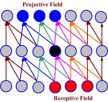
Sensors 2020, 20, 3344                                                                                    2 of 18

computational complexity and consistent performance of the recognition system. It has been suggested
that deep neural architectures are more advantageous than shallow neural architectures [1–6]. The key
differences are described in Table 1. The deep learning field is ever evolving, and some of its variants
are autoencoders, CNNs, recurrent neural networks (RNNs), recursive neural networks, deep belief
networks and deep Boltzmann machines. Here, we introduce a convolutional neural network,
which is a specific type of deep neural network having wide applications in image classification,
object recognition, recommendation systems, signal processing, natural language processing, computer
vision, and face recognition. The ability to automatically detect the important features of an object
(here an object can be an image, a handwritten character, a face, etc.) without any human supervision
or intervention makes them (CNNs) more efficient than their predecessors (Multi layer perceptron
(MLP), etc.). The high capability of hierarchical feature learning results in a highly efficient CNN.

                          Table 1. Shallow neural network vs deep neural network.

               Factors             Shallow Neural Network (SNN)              Deep Neural Network (DNN)
                                 - single hidden layer (need to be fully      - multiple hidden layers (not
    Number of hidden layers
                                                connected).                   necessarily fully connected).
                                       - requires a separate feature
                                                                               - supersedes the handcrafted
                                             extraction process.
                                                                           features and works directly on the
                                 - some of the famous features used in
                                                                                        whole image.
                                    the literature include local binary
       Feature Engineering                                                    - useful in computing complex
                                 patterns (LBPs), histogram of oriented
                                                                               pattern recognition problems.
                                 gradients (HOGs), speeded up robust
                                                                           - can capture complexities inherent
                                 features (SURFs), and scale-invariant
                                                                                         in the data.
                                         feature transform (SIFT).
                                                                            - able to automatically detect the
                                   - emphasizes the quality of features       important features of an object
                                       and their extraction process.         (here an object can be an image,
           Requirements
                                 - networks are more dependent on the        a handwritten character, a face,
                                       expert skills of researchers.             etc.) without any human
                                                                                supervision or intervention.
  Dependency on data volume         - requires small amount of data.         - requires large amount of data.

      A convolutional neural network (CNN) is basically a variation of a multi-layer perceptron (MLP)
network and was used for the first time in 1980 [7]. The computing in CNN is inspired by the human
brain. Humans perceive or identify objects visually. We (humans) train our children to recognize
objects by showing him/her hundreds of pictures of that object. This helps a child identify or make
a prediction about objects he/she has never seen before. A CNN works in the same fashion and is
popular for analyzing visual imagery. Some of the well-known CNN architectures are GoogLeNet
(22 layers), AlexNet (8 layers), VGG (16–19 Ali), and ResNet (152 layers). A CNN integrates the feature
extraction and classification steps and requires minimal pre-processing and feature extraction efforts.
A CNN can extract affluent and interrelated features automatically from images. Moreover, a CNN
can provide considerable recognition accuracy even if there is only a little training data available.
      Design particulars and previous knowledge of features are no longer required to be collected.
Exploitation of topological information available in the input is the key benefit of using a CNN model
towards delivering excellent recognition results. The recognition results of a CNN model are also
independent of the rotation and translation of input images. Contrary to this, thorough topological
knowledge of inputs is not exploited in MLP models. Furthermore, for a complex problem, MLP is not
found to be appropriate, and they do not scale well for higher resolution images because of the full
interconnection between nodes, also called the famous phenomenon of the “curse of dimensionality”.
      In the past few years, the CNN model has been extensively employed for handwritten digit
recognition from the MNIST benchmark database. Some researchers have reported accuracy as good
as 98% or 99% for handwritten digit recognition [8]. An ensemble model has been designed using
a combination of multiple CNN models. The recognition experiment was carried out for MNIST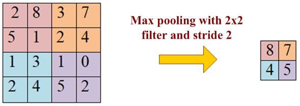
Sensors 2020, 20, 3344                                                                             3 of 18

digits, and an accuracy of 99.73% was reported [9]. Later, this “7-net committee” was extended to
the “35-net committee” experiment, and the improved recognition accuracy was reported as 99.77%
for the same MNIST dataset [10]. An extraordinary recognition accuracy of 99.81% was reported
by Niu and Suen by integrating the SVM (support vector machine) capability of minimizing the
structural risk and the capability of a CNN model for extracting the deep features for the MNIST digit
recognition experiment [11]. The bend directional feature maps were investigated using CNN for in-air
handwritten Chinese character recognition [12]. Recently, the work of Alvear-Sandoval et al. achieved
a 0.19% error rate for MNIST by building diverse ensembles of deep neural networks (DNN) [13].
However, on careful investigation, it has been observed that the high recognition accuracy of MNIST
dataset images is achieved through ensemble methods only. Ensemble methods help in improving the
classification accuracy but at the cost of high testing complexity and increased computational cost for
real-world application [14].
     The purpose of the proposed work is to achieve comparable accuracy using a pure CNN
architecture through extensive investigation of the learning parameters in CNN architecture for
MNIST digit recognition. Another purpose is to investigate the role of various hyper-parameters
and to perform fine-tuning of hyper-parameters which are essential in improving the performance of
CNN architecture.
     Therefore, the major contribution of this work is in two respects. First, a comprehensive evaluation
of various parameters, such as numbers of layers, stride size, kernel size, padding and dilution,
of CNN architecture in handwritten digit recognition is done to improve the performance. Second,
optimization of the learning parameters achieved excellent recognition performance on the MNIST
dataset. The MNIST database has been used in this work because of the availability of its published
results with different classifiers. The database is also popular and mostly used as a benchmark database
in comparative studies of various handwritten digit recognition experiments for various regional and
international languages.
     The novelty of the proposed work lies in the thorough investigation of all the parameters of
CNN architecture to deliver the best recognition accuracy among peer researchers for MNIST digit
recognition. The recognition accuracy delivered in this work employing a fine-tuned pure CNN model
is superior to the recognition accuracies reported by peer researchers using an ensemble architecture.
The use of ensemble architecture by peer researchers involves increased computational cost and high
testing complexity. Hence, the proposed pure CNN model outperforms the ensemble architecture
offered by peer researchers both in terms of recognition accuracy as well as computational complexity.
     The rest of the paper is organized as follows: Section 2 describes the related work in the field
of handwriting recognition; Sections 3 and 4 describe CNN architecture and the experimental setup,
respectively; Section 5 discusses the findings and presents a comparative analysis; and Section 6
presents the conclusion and suggestions for future directions.

2. Related Work
     Handwriting recognition has already achieved impressive results using shallow networks [15–24].
Many papers have been published with research detailing new techniques for the classification of
handwritten numerals, characters and words. The deep belief networks (DBN) with three layers
along with a greedy algorithm were investigated for the MNIST dataset and reported an accuracy of
98.75% [25]. Pham et al. applied a regularization method of dropout to improve the performance
of recurrent neural networks (RNNs) in recognizing unconstrained handwriting [26]. The author
reported improvement in RNN performance with significant reduction in the character error rate (CER)
and word error rate (WER).
     The convolutional neural network brings a revolution in the handwriting recognition field and
delivered the state-of-the-art performance in this domain [27–32]. In 2003, Simard et al. introduced
a general convolutional neural network architecture for visual document analysis and weeded out
the complex method of neural network training [33]. Wang et al. proposed a novel approach for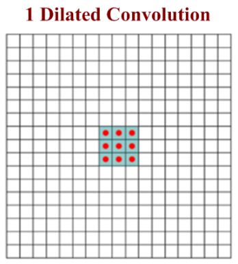
Sensors 2020, 20, 3344                                                                              4 of 18

end-to-end text recognition using multi-layer CNNs and achieved excellent performance on benchmark
databases, namely, ICDAR 2003 and Street View Text [34]. Recently, Shi et al. integrated the advantages
of both the deep CNN (DCNN) and recurrent neural network (RNN) and named it conventional
recurrent neural network (CRNN). They applied CRNN for scene text recognition and found it
to be superior to traditional methods of recognition [35]. Badrinarayanan et al. proposed a deep
convolution network architecture for semantic segmentation. The segmentation architecture is known
as SegNet and consists of an encoder network, a decoder network and a pixel-wise classification layer.
The proposed method used max-pooling indices of a feature map while decoding and observed good
performance. The method is also analyzed and compared with existing techniques for road scene and
indoor understanding [36–38]. CNN has shown remarkable abilities in offline handwritten character
recognition of Arabic language [39]; handwritten Tamil character recognition [40]; Telugu character
recognition [41], handwritten Urdu text recognition [42,43], handwritten character recognition in Indic
scripts [44] and Chinese handwritten text recognition [45–47].
       Recently, Gupta et al. in [48] proposed a novel multi-objective optimization framework for
identifying the most informative local regions from a character image. The work was also evaluated on
isolated handwritten English numerals, namely, MNIST images, along with three other popular Indic
scripts, namely, handwritten Bangala numerals and handwritten Devanagari characters. The authors
used features extracted from a convolutional neural network in their model and achieved 95.96%
recognition accuracy. The work of Nguyen et al. in [49] used a multi-scale CNN for extracting
spatial classification features for handwritten mathematical expression (HME). The local features
and spatial information of HME images were used for clustering HME images. The work observed
high performance for the CROHME dataset. They (authors) also concluded that classification can be
improved by training the CNN with a combination of global max pooling and global attentive pooling.
Ziran et al. [50] developed a faster R-CNN-based framework for text/word location and recognition
in historical books. The authors evaluated these deep learning methods on Gutenberg’s Bible pages.
The handwritten character recognition problem is intelligently addressed in the work of Ptucha et
al. [51] by the introduction of an intelligent character recognition (ICR) system using a conventional
neural network. The work was evaluated on French-based RIMES lexicon datasets and English-based
IAM datasets, showing substantial improvement.
       The performance of CNNs depends mainly on the choice of hyper-parameters [52], which are
usually decided on a trial-and-error basis. Some of the hyper-parameters are, namely, activation
function, number of epochs, kernel size, learning rate, hidden units, hidden layers, etc. These parameters
are very important as they control the way an algorithm learns from data [53]. Hyper-parameters differ
from model parameters and must be decided before the training begins.
       ResNet-52 [54], GoogleNet [55], VGG-16 [56] and AlexNet [57] are some popular CNN models that
have a total of 150, 78, 57 and 27 hyper-parameters, respectively. A bad choice for hyper-parameters
can incur a high computation cost and lead to poor CNN performance. The researcher’s expertise plays
an important role in deciding on the configuration of hyper-parameters and requires an intelligent
strategic plan. This creates several questions about CNN design for handwriting recognition tasks.
How is CNN better in extracting distinct features from handwritten characters? What effect do
different hyper-parameters have on CNN performance? What is the role of design parameters in
improving CNN performance? In order to guide future research in the handwriting recognition field,
it is important to address these questions.

3. Convolutional Neural Network Architecture
     A basic convolutional neural network comprises three components, namely, the convolutional
layer, the pooling layer and the output layer. The pooling layer is optional sometimes. The typical
convolutional neural network architecture with three convolutional layers is well adapted for the
classification of handwritten images as shown in Figure 1. It consists of the input layer, multiple hidden
layers (repetitions of convolutional, normalization, pooling) and a fully connected and an output layer.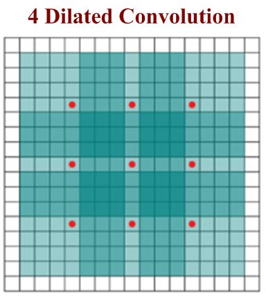
3. Convolutional Neural Network Architecture
A basic convolutional neural network comprises three components, namely, the convolutional
layer, the pooling layer and the output layer. The pooling layer is optional sometimes. The typical
convolutional neural network architecture with three convolutional layers is well adapted for the
Sensors 2020, 20, 3344 5 of 18
classification of handwritten images as shown in Figure 1. It consists of the input layer, multiple
hidden layers (repetitions of convolutional, normalization, pooling) and a fully connected and an
output layer.
Neurons in oneNeurons in one layer
layer connect withconnect
some ofwith some of the
the neurons neurons
present present
in the in themaking
next layer, next layer,
themaking
scaling
the scaling
easier easier
for the for the
higher higher resolution
resolution images. The images. The operation
operation of pooling ofor
pooling or sub-sampling
sub-sampling can be
can be used to
reduce the dimensions of the input. In a CNN model, the input image is considered as a collection ofa
used to reduce the dimensions of the input. In a CNN model, the input image is considered as
collection
small of small
sub-regions sub-regions
called called
the “receptive the “receptive
fields”. fields”.
A mathematical A mathematical
operation operation
of the convolution of the
is applied
convolution
on the input is applied
layer, on the
which input layer,
emulates which emulates
the response thelayer.
to the next response
Theto the nextis
response layer. The response
basically a visual
is basicallyThe
stimulus. a visual stimulus.
detailed The detailed
description description is as follows:
is as follows:
3.1. Input layer
Layer
The input data is loaded and stored in the input layer.
layer. This layer describes the height, width and
number of channels (RGB information)
information) of
of the
the input
input image.
image.
Figure 1. Typical convolutional neural network architecture.
Figure 1. Typical convolutional neural network architecture.
3.2. Hidden Layer
3.2. Hidden Layer layers are the backbone of CNN architecture. They perform a feature extraction
The hidden
process
Thewhere a series
hidden layersofare
convolution, pooling
the backbone and activation
of CNN functions
architecture. They are used. aThe
perform distinguishable
feature extraction
features of handwritten digits are detected at this stage.
process where a series of convolution, pooling and activation functions are used. The distinguishable
features of handwritten digits are detected at this stage.
3.3. Convolutional Layer
3.3. Convolutional
The convolutional Layer layer is the first layer placed above the input image. It is used for extracting
the features of an image.
The convolutional Theisnthe
layer × nfirst
input neurons
layer placedofabove
the input layer image.
the input are convoluted
It is usedwith an m × m
for extracting
filter and in return
the features deliverThe
of an image. (n − m × + 1)
input − m + 1)ofasthe
× (nneurons output.
inputItlayerintroduces non-linearity
are convoluted with an through × a
neural activation function. The main contributors of the convolutional
filter and in return deliver ( − + 1) × ( − + 1) as output. It introduces non-linearity through layer are receptive field, stride,
dilation
a neuraland padding,
activation as described
function. in thecontributors
The main following paragraph.
of the convolutional layer are receptive field,
CNN computation is inspired by the
stride, dilation and padding, as described in the following visual cortex in animals
paragraph. [58]. The visual cortex is a part of
the brain that processes the information forwarded
CNN computation is inspired by the visual cortex in animals [58]. from the retina. It processes visualcortex
The visual information
is a partand
of
is
thesubtle
braintothatsmall sub-regions
processes of the input.forwarded
the information Similarly, afrom receptive field isItcalculated
the retina. processes in a CNN,
visual which is
information
aand
small regiontoofsmall
is subtle an input image that
sub-regions of can affect aSimilarly,
the input. specific region of the field
a receptive network. It is also in
is calculated one of the
a CNN,
important
which is a small region of an input image that can affect a specific region of the network. It is also [59].
design parameters of the CNN architecture and helps in setting other CNN parameters one
It has the same size as the kernel and works in a similar fashion
of the important design parameters of the CNN architecture and helps in setting other CNN as the foveal vision of the human eye
works for producing sharp central vision. The receptive field is influenced
parameters [59]. It has the same size as the kernel and works in a similar fashion as the foveal vision by striding, pooling, kernel
size
of theand depth eye
human of the CNNfor
works [60]. Receptivesharp
producing field (r), effective
central receptive
vision. field (ERF)
The receptive andisprojective
field influenced field
by
(PF) are terminology used in calculating effective sub-regions in a network.
striding, pooling, kernel size and depth of the CNN [60]. Receptive field (r), effective receptive field The area of the original
image
(ERF) and influencing
projective the activation
field (PF) areof a neuron isused
terminology described using the
in calculating ERF, whereas
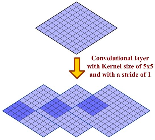
effective sub-regions the PFin aisnetwork.
a count
of
The neurons
area oftothe which neurons
original image project their outputs,
influencing as described
the activation in Figure
of a neuron is 2.described
The visualization
using theofERF, the
× 5-size the
5whereas filterPFandis a count of neurons to which neurons project their outputs, as described in
its activation map are described in Figure 3. Stride is another parameter used in
CNN architecture.
Figure 2. The visualization It is defined as the
of the 5 × step
5-size size by and
filter which itsthe filter moves
activation map every time. A stride
are described value
in Figure 3.
of 1 indicates the filter sliding movement pixel by pixel. A larger stride
Stride is another parameter used in CNN architecture. It is defined as the step size by which the filter size shows less overlapping
between the cells. The working of kernel and stride in the convolution layer is presented in Figure 4.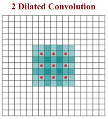
Sensors 2020, 20, x FOR PEER REVIEW 6 of 18
Sensors 2020, 20, x FOR PEER REVIEW 6 of 18
moves every
Sensors 2020, 20, xtime. A stride
FOR PEER value of 1 indicates the filter sliding movement pixel by pixel. A larger
REVIEW 6 of 18
stride size shows less overlapping between the cells. The working of kernel and stride
moves every time. A stride value of 1 indicates the filter sliding movement pixel by pixel. A larger in the
moves everylayer
convolution time.isApresented
stride value
in of 1 indicates
Figure 4. the filter sliding movement pixel by pixel. A larger
stride2020,
Sensors size20,shows
3344 less overlapping between the cells. The working of kernel and stride in 6 ofthe
18
stride size shows less overlapping between the cells. The working of kernel and stride in the
convolution layer is presented in Figure 4.
convolution layer is presented in Figure 4.
Figure 2. Receptive field and projective field.
Figure 2. Receptive field and projective field.
Figure 2. Receptive
Receptive field
field and
and projective
projective field.
Figure 3. Visualization of filter of size 5 × 5 with activation map. (Input neuron 28 × 28 and
Figure 3. Visualization
convolutional filter of size 5 × 5 with activation map. (Input neuron 28 × 28 and convolutional
layer 24 ×of24).
Figure 3. Visualization of filter of size 5 × 5 with activation map. (Input neuron 28 × 28 and
layer 243.× Visualization
Figure 24). of filter of size 5 × 5 with activation map. (Input neuron 28 × 28 and
convolutional layer 24 × 24).
convolutional layer 24 × 24).
Figure 4. Representation of kernel and stride in a convolutional layer.
Figure 4. Representation of kernel and stride in a convolutional layer.
The concept ofFigurepadding is introduced
4. Representation in CNN
of kernel andarchitecture to get more
stride in a convolutional accuracy. Padding is
layer.
The concept
introduced ofFigure
to control padding
the 4. is introduced
Representation
shrinking of the of in CNN
kernel
output and
of architecture
thestride to get
in a convolutional
convolutional more
layer. accuracy. Padding is
layer.
introduced
The to control
The output
concept from the
the shrinking
of paddingconvolutionalof the
is introduced output
layer in of
is aCNN thearchitecture
feature convolutional
map, which to islayer.
get more than
smaller accuracy. Padding
the input image. is
The output
conceptfrom of padding
the is introduced
convolutional layer in
is CNN
a architecture
feature map, which to is
get more than
smaller accuracy.
the Padding
input image. is
introduced
The to control
output feature mapthe shrinking
contains moreofinformation
the output of onthe convolutional
middle pixels and layer.
hence loses lots of information
introduced
The output tofeature
controlmap
the shrinking
contains of the output of the convolutional layer.and hence loses lots of
Theonoutput
present corners.fromThethe
rows and themore
convolutional columns information
layer is
ofazeros
feature on
are middle
map,
added which pixels
to the isborder
smallerofthan the input
an image image.
to prevent
The output
information fromon
present thecorners.
convolutional
The layer
rows and is athe
feature
columnsmap,ofwhich
zeros isare
smaller
added than
to the border
the input image.
of an
The output feature map
shrinking of the feature map. contains more information on middle pixels and hence loses lots of
The output
image to feature
prevent map contains
shrinking of the moremap.
feature information on middle pixels and hence loses lots of
information
Equations present
(1) andon (2)corners.
describeThethe rows and thebetween
relationship columns theofsize
zeros arefeature
of the added map,
to thethe
border
kernelofsize
an
information
Equations present on(2)corners. Thethe
rows and the columns of
thezeros arethe
added to the border of an
image
and stride while(1)calculating
to prevent and
shrinking describe
of
thethe relationship
feature
size of the map.
output feature betweenmap. size of feature map, the kernel
image
size andtostride
prevent shrinking
while of thethe
calculating feature ofmap.
sizerelationship
the outputbetween
feature map.
Equations (1) and (2) describe the the size of the feature map, the kernel
Equations (1) and (2) describe the relationship
Wnx of = the
Wn−1x between
Snx +the
− Fnxfeature 1map.size of the feature map, the kernel (1)
size and stride while calculating the size output
size and stride while calculating the size of the output feature map.
Wny = Wn−1y − Fny Sny + 1 (2)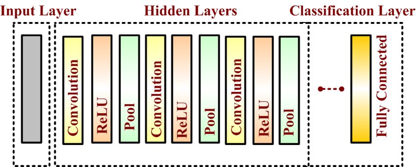
Sensors 2020, 20, x FOR PEER REVIEW 7 of 18
Sensors 2020, 20, x FOR PEER REVIEW 7 of 18
Sensors 2020, 20, 3344 7 of 18
= − +1 (1)
= − +1 (1)
where (Wnx , Wny ) represent the size of the= −
output feature map,+ 1(Snx , Sny ) is stride size, and (Fx , F y(2) ) is
= − +1 (2)
kernel
where ( size. , Here ‘n’ is used to describe the index of
) represent the size of the output feature map, ( , layers. )is stride size, and ( , ) is
where (
The ,
dilation ) represent
is another the size
important of the output
parameter
kernel size. Here ‘n’ is used to describe the index of layers. feature
of CNN map, (
architecture , )is stride
that size, and
has a direct ( , )on
influence is
kernel
the size.
receptive
The Here
field.‘n’
dilation isTheis used
another to
dilation describe the index
can increase
important of
of layers.
the field-of-view
parameter (FOV) of athat
CNN architecture CNN haswithout
a directmodifying
influencetheon
the receptive field. The dilation can increase the field-of-view (FOV) of a CNN withoutinfluence
The
feature dilation
map [61]. is another
Figure 5 important
clearly shows parameter
that dilationof CNN
values architecture
can that
exponentially has a
raise direct
the receptive on
field
modifying
theafeature
of
the receptive
CNN. Too map field.
[61].The
large dilation
aFigure
dilation cancanincrease
5 clearly increase
shows thethatthe field-of-view
number
dilation of (FOV)
computations
values of aand
can exponentiallyCNN without
hence canthe
raise modifying
slow down
receptive
the feature
system map
by [61].
increasingFigurethe 5 clearly
processing shows that
time. dilation
Therefore, values
it must can
be
field of a CNN. Too large a dilation can increase the number of computations and hence can slow exponentially
chosen wisely. raise
The the receptive
relationship
field ofthe
between
down adilation,
CNN.
system Too bylarge
weight anda dilation
increasinginputthe is can
shownincrease the number
in Equations
processing time. of computations
(3) and
Therefore, (4)itbelow. and hence
must be chosen can slow
wisely. The
down the system
relationship between bydilation,
increasing the and
weight processing
input is time.
shownTherefore,
in Equations it must
(3) and be(4)chosen
below.wisely. The
relationship between dilation, weight=and
0 − dialation w[0input
] ∗ x[0is
] +shown
w[1] ∗ in
x[1Equations
] + w[2] ∗ x(3) [2];and (4) below. (3)
0− = [0] ∗ [0] + [1] ∗ [1] + [2] ∗ [2]; (3)
0− 1 − dialation = = w[0]
[0] ∗∗ x[[0]
0] ++w[1[1]
] ∗ ∗x[2[1]
] ++ w[2][2]
∗ x∗[4];[2]; (3)
(4)
1− = [0] ∗ [0] + [1] ∗ [2] + [2] ∗ [4]; (4)
1− = [0] ∗ [0] + [1] ∗ [2] + [2] ∗ [4]; (4)
(a) (b) (c)
(a) (b) (c)
Figure 5. Dilated convolution: (a) receptive field of 3 × 3 using 1-dilated convolution; (b) receptive
Figure 5. Dilated
Dilated convolution: (a) receptive field
field of
of 33 ×× 33 using
using 1-dilated convolution;
convolution; (b)
(b) receptive
receptive
Figure
field of5.7 × 7 usingconvolution: (a) receptive
2-dilated convolution; (c) receptive field of 15 1-dilated
× 15 using 4-dilated convolution.
field of
field of 77 ×
× 77 using
using 2-dilated
2-dilated convolution; (c) receptive
convolution; (c) receptive field
field of
of 15
15 ×
× 15
15 using
using 4-dilated
4-dilated convolution.
convolution.
3.4. Pooling Layer
3.4. Pooling Layer
3.4. Pooling Layer
A pooling layer is added between two convolutional layers to reduce the input dimensionality
A
A pooling
pooling layer
layeristhe
isadded
added between
between two
twoconvolutional
convolutional layers to reduce
layers to reducethe the
input dimensionality
input dimensionality and
and hence to reduce computational complexity. Pooling allows the selected values to be passed
hence
and to reduce the computational complexity. Pooling allows the selected valuesvalues
to be passed to the
to thehence to reduce
next layer whilethe computational
leaving complexity.
the unnecessary valuesPooling
behind.allows the selected
The pooling layer also helps to be passed
in feature
next layer
to the nextandwhile
layer leaving the unnecessary values behind. The pooling layer also helps in feature selection
selection in while leaving
controlling the unnecessary
overfitting. valuesoperation
The pooling behind. The pooling
is done layer also helps
independently. in feature
It works by
and in controlling
selection and in overfitting.
controlling The pooling
overfitting. Theoperation
pooling is done independently.
operation is done It works byItextracting
independently. worksThe by
extracting only one output value from the tiled non-overlapping sub-regions of the input images.
only one output
extractingtypesonly one value from the tiled non-overlapping sub-regions of the input images. The common
common of output
poolingvalue from theare
operations tiled non-overlapping
max-pooling and sub-regions
avg-poolingof(where the input
max images.
and Theavg
types
common of pooling
types operations
of pooling are max-pooling
operations are and avg-pooling
max-pooling (where
and max and (where
avg-pooling avg represent
max maxima
and avg
represent maxima and average, respectively). The max-pooling operation is generally favorable in
and average,
represent respectively).
maxima and The max-pooling
average, respectively). operation
The is generallyoperation
max-pooling favorableisingenerally
modern applications,
favorable in
modern applications, because it takes the maximum values from each sub-region, keeping maximum
because it takes
modern applications, the maximum
because values
it takes from each
the maximumsub-region, keeping maximum information. This leads
information. This leads to faster convergence andvalues
betterfrom each sub-region,
generalization [62]. keeping maximum
The max-pooling
to faster convergence
information. This and better
leads to generalization
faster convergence [62].
andThebetter
max-pooling operation
generalization for converting
[62]. The a4×4
max-pooling
operation for converting a 4 × 4 convolved output into a 2 × 2 output with stride size 2 is described in
convolved
operation output
for into a 2 ×42×output
converting with stride size 2 isadescribed in Figure 6. The maximum number
Figure 6. The maximum anumber 4 convolved
is taken output
from eachinto 2 × 2 output
convolved with (of
output stride
sizesize
2 ×2 2)
is described
resulting in in
is taken from
Figure 6. the each
Theoverall convolved
maximum output
number (of size 2 × 2) resulting in reducing the overall size to 2 × 2.
reducing size to 2 × 2. is taken from each convolved output (of size 2 × 2) resulting in
reducing the overall size to 2 × 2.
Figure 6. Max pooling with filter 2 × 2 and stride size.
Figure 6. Max pooling with filter 2 × 2 and stride size.
Figure 6. Max pooling with filter 2 × 2 and stride size.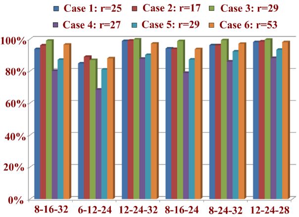
Sensors 2020, 20, 3344                                                                                         8 of 18

3.5. Activation Layer
     Just like regular neural network architecture, CNN architecture also contains the activation
function to introduce the non-linearity in the system. The sigmoid function, rectified linear unit (ReLu)
and Softmax are some famous choices among various activation functions exploited extensively in
deep learning models. It has been observed that the sigmoid activation function might weaken the
CNN model because of the loss of information present in the input data. The activation function used
in the present work is the non-linear rectified linear unit (ReLu) function, which has output 0 for
input less than 0 and raw output otherwise. Some advantages of the ReLu activation function are its
similarity with the human nerve system, simplicity in use and ability to perform faster training for
larger networks.

3.6. Classification Layer
     The classification layer is the last layer in CNN architecture. It is a fully connected feed forward
network, mainly adopted as a classifier. The neurons in the fully connected layers are connected to all
the neurons of the previous layer. This layer calculates predicted classes by identifying the input image,
which is done by combining all the features learned by previous layers. The number of output classes
depends on the number of classes present in the target dataset. In the present work, the classification
layer uses the ‘softmax’ activation function for classifying the generated features of the input image
received from the previous layer into various classes based on the training data.

3.7. Gradient Descent Optimization Algorithm
     Optimization algorithms are used to optimize neural networks and to generate better performance
and faster results. The algorithm helps in minimizing or maximizing a cost function by updating
the weight/bias values, which are known as learning parameters of a network, and the algorithm
updating these values is termed as the adaptive learning algorithm. These learning parameters directly
influence the learning process of a network and have an important role in producing an efficient
network model. The aim of all the optimization algorithms is to find the optimum values of these
learning parameters. The gradient descent algorithm is one such optimization algorithm. Recent
classification experiments based on deep learning reported excellent performance with the progress in
learning parameter identification [63–69].
     Gradient descent, as the name implies, uses an error gradient to descend along with the error
surface. It also allows a minimum of a function to be found when a derivative of it exists and there is
only one optimum solution (if we expect local minima). The gradient is the slope of the error surface
and gives an indication of how sensitive the error is towards the change in the weights. This sensitivity
can be exploited for incremental change in the weights towards the optimum. Gradient descent is
classified into three types, namely, batch gradient descent, stochastic gradient descent (SGD) and
mini-batch gradient descent.
     The SGD algorithm works faster and has been extensively used in deep learning
experiments [70–74]. The SGD algorithm avoids redundant computation better than the batch gradient
descent algorithm. The algorithm steps for updating the learning parameter for each training data bit
are as follows (Algorithm 1):

 Algorithm 1 Learning Parameters Update Mechanism
 1: Input: (x(i), y(i)) as training data; η as learning rate; ∇E(θ) is a gradient of loss (error) function E(θ) with
 respect to the θ parameter; momentum factor (m)
 2: Output: For each training pair, update the learning parameters using the equation
 θ=θ-η.∇E(θ;x(i);y(i))
 3: if stopping condition is met
 4: return parameter θ.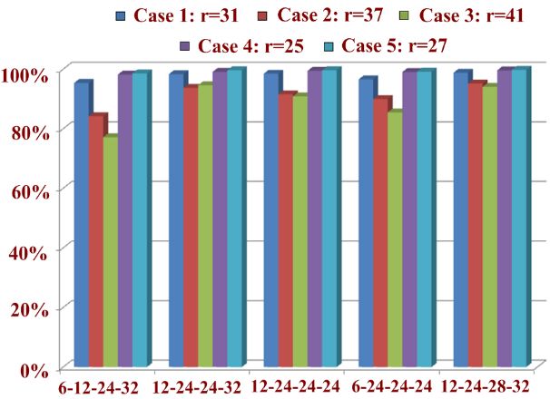
Sensors 2020, 20, 3344                                                                               9 of 18

     The SGD algorithm can be further optimized using various optimizers, such as momentum,
adaptive moment estimation (Adam), Adagrad and Adadelta. The momentum parameter is selected to
speed up SGD optimization. The momentum optimizer can reduce the unnecessary parameter update,
which leads to faster convergence of the network. The modified update equations with the momentum
factor (m) are given by (5).
                                      z(t) = mz(t − 1) + η∇E(θ)
                                                                )
                                                                                               (5)
                                             θ = θ − z(t)
     Most implementation usually considers m = 0.9 for updating the learning parameters.
     Adagrad is one of the SGD algorithms widely preferred in optimizing sparse data. The Adagrad
optimizer works by considering the past gradients and modifying the learning rate for every parameter
at each time step. The update equation for the Adagrad optimizer is given by (6).
                                                         η
                                      θt+1,i = θt,i − p           .gt,i                                 (6)
                                                       Gt, ii + ε

where g(t, i) is a gradient of the loss function for parameter θ(i) at a time step t; ε is a smoothing term
taken to avoid the division by 0; and Gt, ii is a diagonal matrix representing the sum of gradient squares
for parameter θ(i) for a time step t;
      The learning rate in the Adagrad optimizer keeps on decreasing, which causes a slow convergence
rate and longer training time. Adadelta is another adaptive learning algorithm and is an extension
of the Adagrad optimizer. It can beat the decaying learning rate problem of the previous optimizer,
i.e., Adagrad [61]. Adadelta limits the storage of past squared gradients by fixing the storage window
size. The moving averages of the square of gradients and square of weights updates are calculated.
The learning
           h irate is basically the square root of the ratio between these moving averages. A running
average E g2 at time step t of the past gradient is calculated using (7).
                 t
                                      h i     h i
                                     E g2 = γE g2             + (1 − γ) g2t                             (7)
                                           t            t−1

where I _ is similar to the momentum term.
    The parameter update for Adadelta optimization is done using Equations (8) and (9).

                                                 ∆θt = −η.gt,i                                          (8)

                                               ∆θt+1 = θt + ∆θt                                         (9)

or (10) can be modified as
                                                    η
                                          ∆θt = − √                 gt                                (10)
                                                   Gt + ε
                                                              h i
      Replacing the diagonal matrix with the running average E g2 ,
                                                                              t

                                                     η
                                        ∆θt = − q                        gt                           (11)
                                                 E[ g2 ]t + ε

                                                       η
                                          ∆θt = −                   gt                                (12)
                                                     RMS[ g]t
where RMS[ g]t is the parameter update root mean square error and is calculated using (13):
                                                       q
                                         RMS[ g]t =     E[ g2 ]t + ε                                  (13)

    Adam is another famous SGD optimizer having learning weight updating similar to the storing
average in Adadelta and decaying average of past squared gradients as present in the momentum
Sensors 2020, 20, 3344 10 of 18
optimizer. Adam outperforms other techniques by performing fast convergence with a fast learning
speed. Equations (14) and (15) are used to calculate the first-moment value (M(t)) and the variance of
gradients (v(t)):
mt
m̂t = (14)
1 − βt1
vt
v̂t = (15)
1 − βt2
and the parameter update is given in Equation (16):
η
θt+1 = θt − √ m̂t (16)
v̂t + ε
4. Experimental Setup
To accomplish the task of handwritten digit recognition, a model of the convolutional neural
network is developed and analyzed for suitable different learning parameters to optimize recognition
accuracy and processing time. We propose to investigate variants of CNN architecture with three
layers (CNN_3L) and variants of CNN architecture with four layers (CNN_4L). A total of six cases
(case 1 to case 6) have been considered for CNN with three-layer architecture and five cases (case 1 to
case 5) for CNN architecture with four layers. All the cases differ in the number of feature maps, stride
sizes, padding, dilation and received receptive fields.
The recognition process of the handwritten digits consists of the following steps:
1. To acquire or collect the MNIST handwritten digit images.
2. To divide the input images into training and test images.
3. To apply the pre-processing technique to both the training dataset and the test dataset.
4. To normalize the data so that it ranges from 0 to 1.
5. To divide the training dataset into batches of a suitable size.
6. To train the CNN model and its variants using the labelled data.
7. To use a trained model for the classification.
8. To analyze the recognition accuracy and processing time for all the variants.
In summary, the present work for handwritten digit recognition investigates the role of training
parameters, gradient descent optimizers and CNN architecture.
All the experiments were done in MATLAB 2018b on a personal computer with Windows 10,
Intel (R) Core (TM) i7-6500 CPU (2.50 GHz), 16.00 GB memory and NVIDIA 1060 GTX GPU. The MNIST
database was involved in the training and testing models. The standard MNIST handwritten digit
database has 60,000 and 10,000 normalized digit images in its training and testing datasets, respectively.
Some of the sample images from the MNIST database are shown in Figure 7.
Data pre-processing plays an important role in any recognition process. To shape the input images
in a form suitable for segmentation, the pre-processing methods, such as scaling, noise reduction,
centering, slanting and skew estimation, were used. In general, many algorithms work better after the
data has been normalized and whitened. One needs to work with different algorithms in order to find
out the exact parameters for data pre-processing. In the present work, the MNIST dataset images were
size-normalized into a fixed image of size 28 × 28.
A convolution layer with 28 kernel/filter/patches and kernel sizes of 5 × 5 and 3 × 3 is used here
to extract the features. Every patch contains the structural information of an image. For example,
a convolution operation is computed by sliding a filter of size 5 × 5 over input image. This layer is
responsible for transforming the input data by using a patch/filter of locally connecting neurons from
the previous layer.parameters, gradient descent optimizers and CNN architecture.
All the experiments were done in MATLAB 2018b on a personal computer with Windows 10,
Intel (R) Core (TM) i7-6500 CPU (2.50 GHz), 16.00 GB memory and NVIDIA 1060 GTX GPU. The
MNIST database was involved in the training and testing models. The standard MNIST handwritten
Sensors
digit 2020, 20, has
database 3344 60000 and 10000 normalized digit images in its training and testing datasets,
11 of 18
respectively. Some of the sample images from the MNIST database are shown in Figure 7.
Figure
Figure 7.
7. Sample
Sample MNIST
MNIST handwritten
handwritten digit
digit images.
images.
Data pre-processing plays an important role in any recognition process. To shape the input
5. Results and Discussion
images in a form suitable for segmentation, the pre-processing methods, such as scaling, noise
Thecentering,
reduction, experimental results
slanting andofskew
the MNIST handwritten
estimation, were used.digit
In dataset
general,using
manydifferent parameters
algorithms work
of CNN_3L and CNN_4L architectures are recorded and analyzed in Tables 2 and 3, respectively.
better after the data has been normalized and whitened. One needs to work with different algorithms
An MNIST sample image is represented as a 1-D array of 784 (28 × 28) float values between 0 and 1
in order to find out the exact parameters for data pre-processing. In the present work, the MNIST
(0 stands for black, 1 for white). The receptive field (r) is calculated based on kernel size (k), stride (s),
dataset images
dilation were size-normalized
(d), padding (p), input size into
(i/p)aand
fixed imagesize
output of size
(o/p)28of×the
28.feature map, and the recognition
A convolution
accuracy and totallayer
time with 28 kernel/filter/patches
elapsed is shown in Tables 2 and and3,kernel sizes CNN
employing of 5 × architecture
5 and 3 × 3 is used
with here
three and
to four
extract the features.
layers Every
respectively. Thepatch contains
findings the 2structural
of Table confirm theinformation of an image.
role of different For example,
architecture a
parameters
convolution operation is computed by sliding a filter of size 5 × 5 over input
on the performance of our recognition system. The training parameter used here has a learning image. This layer is
responsible forand
rate of 0.01 transforming
maximumthe input
epoch data by
counts of using
4. Thea patch/filter of locallyaccuracy
highest recognition connecting neuronsinfrom
achieved case 3,
thewith
previous layer.architecture having three layers, is 99.76% for the feature map 12-24-32. In case 5,
CNN_3L
the CNN_4L architecture with four layers achieved the highest recognition accuracy of 99.76 % for the
feature map 12-24-28-32, as shown in Table 3.
Table 2. Configuration details and accuracy achieved for convolutional neural network with three layers.
Recognition Accuracy (%) and Total Time Elapsed
Model Layer k s d p i/p o/p r
8-16-32 6-12-24 12-24-32 8-16-24 8-24-32 12-24-28
Layer 1 5 2 2 2 28 14 5
93.76% 84.76% 98.76% 94.08% 96.12% 98.08%
Case 1 Layer 2 5 2 1 2 14 7 9
(20 s) (42 s) (45 s) (46 s) (42 s) (44 s)
Layer 3 5 2 1 2 7 4 25
Layer 1 5 2 1 2 28 14 5
96.04% 88.91% 99% 93.80% 96.12% 98.48%
Case 2 Layer 2 3 2 1 2 14 7 9
(37 s) (27 s) (37 s) (37 s) (37 s) (17 s)
Layer 3 3 2 1 2 7 4 17
Layer 1 5 2 1 2 28 14 5
98.96% 86.88% 99.7% 98.72% 99.28% 99.60%
Case 3 Layer 2 5 2 1 2 14 7 13
(27 s) (27 s) (29 s) (39 s) (31 s) (53 s)
Layer 3 5 2 1 2 7 4 29
Layer 1 3 3 1 1 28 10 3
80.16% 68.40% 87.72% 78.84% 85.96% 88.16%
Case 4 Layer 2 3 3 1 1 10 4 9
(48 s) (29 s) (29 s) (29 s) (51 s) (29 s)
Layer 3 3 3 1 1 4 2 27
Layer 1 5 3 1 2 28 10 5
87.08% 80.96% 90.08% 87.22% 92.24% 93.32%
Case 5 Layer 2 3 3 1 1 10 4 11
(52 s) (30 s) (24 s) (24 s) (24 s) (24 s)
Layer 3 3 3 1 1 4 2 29
Layer 1 5 3 1 2 28 10 5
96.48% 87.96% 97.16% 93.68% 97.04% 98.06%
Case 6 Layer 2 5 3 1 2 10 4 17
(23 s) (23 s) (23 s) (24 s) (24 s) (24 s)
Layer 3 5 3 1 2 4 2 53Sensors 2020, 20, 3344 12 of 18
Table 3. Configuration details and accuracy achieved for convolutional neural network with four layers.
Recognition Accuracy (%) and Total Time Elapsed
Model Layer k s d p i/p o/p r
6-12-24-32 12-24-24-32 12-24-24-24 6-24-24-24 12-24-28-32
Layer 1 3 2 1 1 28 14 3
Layer 2 3 2 1 1 14 7 7 95.36% 98.34% 98.48% 96.56% 98.80%
Case 1
Layer 3 3 2 1 1 7 4 15 (56 s) (31 s) (53 s) (44 s) (31 s)
Layer 4 3 2 1 1 4 2 31
Layer 1 3 2 2 2 28 14 5
Layer 2 3 2 2 2 14 7 13 84.20% 93.72% 91.56% 89.96% 95.16%
Case 2
Layer 3 3 2 1 1 7 4 21 (26 s) (30 s) (24 s) (26 s) (25 s)
Layer 4 3 2 1 1 4 2 37
Layer 1 5 2 2 2 28 14 9
Layer 2 3 2 2 2 14 7 17 77.16% 94.60% 90.88% 85.48% 94.04%
Case 3
Layer 3 3 2 1 1 7 4 25 (32 s) (25 s) (26 s) (25 s) (26 s)
Layer 4 3 2 1 1 4 2 41
Layer 1 5 1 2 2 28 17 9
Layer 2 3 2 2 2 17 7 13 98.20% 99.12% 99.44% 99.04% 99.60%
Case 4
Layer 3 3 2 1 1 7 4 17 (30 s) (29 s) (25 s) (22 s) (29 s)
Layer 4 3 2 1 1 4 2 25
Layer 1 5 1 2 2 28 28 9
Layer 2 5 2 1 2 28 14 13 98.60% 99.64% 99.64% 99.20% 99.76%
Case 5
Layer 3 3 2 1 1 14 7 17 (27 s) (27 s) (27 s) (27 s) (43 s)
Sensors 2020, 20, x FOR PEER REVIEW 13 of 18
Layer 4 3 2 1 1 7 4 27
Layer 2 5 2 1 2 28 14 13
98.60% 99.64% 99.64% 99.20% 99.76%
Layer 3 3 2 1 1 14 7 17
The values of different architectural parameters have
(27 s) been
(27chosen
s) in(27
such
s) a way
(27as
s) to observe
(43 s) the
Layer 4 3 2 1 1 7 4 27
role of all the parameters. For all convolutional layers, the hyper-parameters include kernel size (1–5),
The values of different architectural parameters have been chosen in such a way as to observe
stride (1–3), dilation (1–2) and padding (1–2). The first observation from both of the tables shows the
the role of all the parameters. For all convolutional layers, the hyper-parameters include kernel size
role of the receptive field. The value of the receptive field, when close to the input size, observed good
(1–5), stride (1–3), dilation (1–2) and padding (1–2). The first observation from both of the tables
recognition
shows theaccuracy
role of theforreceptive
all the feature maps
field. The value(case 3 inreceptive
of the Table 2 andfield,case
when5 in Table
close to 3).
the On
inputthesize,
other
hand, a large
observed gaprecognition
good between receptive
accuracyfield and
for all theinput
featuresize observed
maps (case 3 poor recognition
in Table 2 and caseaccuracy
5 in Table (case
3). 3
and case 6 in Table 2 and case 3 in Table 3). The plots of Figure 8a,b clearly
On the other hand, a large gap between receptive field and input size observed poor recognition describe the relationship
between
accuracyrecognition
(case 3 andaccuracy
case 6 inand receptive
Table field.3 in
2 and case This highlights
Table that receptive
3). The plots of Figurefield
8a,b can easily
clearly capture
describe
thetheelementary
relationship information like edgesaccuracy
between recognition and corners from thefield.
and receptive input images
This in thethat
highlights lower layersfield
receptive of the
CNN, which is passed to the subsequent layers for further processing. From
can easily capture the elementary information like edges and corners from the input images in theTables 2 and 3, it can also
be lower
observed
layersthat an increased
of the CNN, which number of filters
is passed to the (or increased
subsequent width
layers forof the CNN)
further helps From
processing. in improving
Table
the2 performance
and Table 3, itofcanCNN alsoarchitecture.
be observed Case
that an increased
5 of Table 3 number of filters (orthe
also demonstrates increased width
capability of the
of multiple
CNN)
filters helps in improving
in extracting the performance
the full features of CNN architecture.
of the handwritten images. Case 5 of Table 3 also demonstrates
the capability of multiple filters in extracting the full features of the handwritten images.
(a) Three-layer CNN model architecture vs. percentage accuracy (b) Four-layer CNN model architecture vs. percentage
accuracy
Figure Receptive
8. 8.
Figure Receptivefields
fieldsand
andrecognition
recognition accuracies forCNN:
accuracies for CNN:(a)
(a)architecture
architecturehaving
having three
three layers;
layers;
(b)(b)
architecture having
architecture havingfour
fourlayers.
layers.
The recognition accuracy of MNIST handwritten digits with different optimizers is shown in
Table 4. The optimizers like stochastic gradient descent with momentum (SGDm), Adam, Adagrad
and Adadelta are used in the present work to obtain optimized performance. The highest accuracy is
achieved using CNN_3L architecture with an Adam optimizer. The Adam optimizer computesSensors 2020, 20, 3344 13 of 18
The recognition accuracy of MNIST handwritten digits with different optimizers is shown in
Table 4. The optimizers like stochastic gradient descent with momentum (SGDm), Adam, Adagrad
and Adadelta are used in the present work to obtain optimized performance. The highest accuracy
is achieved using CNN_3L architecture with an Adam optimizer. The Adam optimizer computes
adaptive learning rates for each parameter and performs fast convergence. It can be observed that
training with the optimizer increases the accuracy of the classifier in both cases involving CNN_3L
and CNN_4L. Furthermore, the optimized CNN variant having four layers has less accuracy than
the similar variants with three layers. The increased number of layers might cause overfitting and
consequently can influence the recognition accuracy. The problem of the overfitting can be avoided by
finding out optimal values using trial and error or under some guidance. The concept of dropout may
be used to solve the problem of overfitting, in which we can stop some randomly selected neurons
(both hidden and visible) from participating in the training process. Basically, dropout is a weight
regularization technique and is most preferred in larger networks to achieve better outcomes. Generally,
a small value of dropout is preferred; otherwise, the network may be under learning.
The objective of the present work is to thoroughly investigate all the parameters of CNN
architecture that deliver best recognition accuracy for a MNIST dataset. Overall, it has been observed
that the proposed model of CNN architecture with three layers delivered better recognition accuracy
of 99.89% with the Adam optimizer.
Table 4. Recognition accuracy with different optimizers.
Recognition Accuracy (%)
Model Momentum
Adam Adagrad Adadelta
(Sgdm)
CNN_3L 99.76% 99.89 98.67 99.77
CNN_4L 99.76% 99.35 98 99.73
The comparison of the proposed CNN-based approach with other approaches for handwritten
numeral recognition is provided in Table 5. It can be observed that our CNN model outperforms
the various similar CNN models proposed by various researchers using the same MNIST benchmark
dataset. Some researchers used ensemble CNN architectures for the same dataset to improve their
recognition accuracy but at the cost of increased computational cost and high testing complexity.
The proposed CNN model achieved recognition accuracy of 99.89% for the MNIST dataset even
without employing ensemble architecture.
Table 5. Comparison of proposed CNN architecture for numeral recognition with other techniques.
Handwritten Numeral Recognition
Accuracy
Reference Approach Database Features
(%)/Error Rate
[75] CNN MNIST Pixel based 0.23%
[76] CNN MNIST Pixel based 0.19%
[8] CNN MNIST Pixel based 0.53%
[77] CNN MNIST Pixel based 0.21%
[78] CNN MNIST Pixel based 0.17%
88.89% (GoogleNet)
[79] Deep Learning The Chars74K Pixel based
77.77% (Alexnet)
Urdu Nasta’liq
Pixel and
[43] CNN handwritten 98.3%
geometrical based
dataset (UNHD)
Pixel and
Proposed approach CNN MNIST 99.89%
geometrical basedSensors 2020, 20, 3344 14 of 18
6. Conclusions
In this work, with the aim of improving the performance of handwritten digit recognition,
we evaluated variants of a convolutional neural network to avoid complex pre-processing, costly
feature extraction and a complex ensemble (classifier combination) approach of a traditional recognition
system. Through extensive evaluation using a MNIST dataset, the present work suggests the role
of various hyper-parameters. We also verified that fine tuning of hyper-parameters is essential in
improving the performance of CNN architecture. We achieved a recognition rate of 99.89% with
the Adam optimizer for the MNIST database, which is better than all previously reported results.
The effect of increasing the number of convolutional layers in CNN architecture on the performance of
handwritten digit recognition is clearly presented through the experiments.
The novelty of the present work is that it thoroughly investigates all the parameters of CNN
architecture that deliver best recognition accuracy for a MNIST dataset. Peer researchers could not
match this accuracy using a pure CNN model. Some researchers used ensemble CNN network
architectures for the same dataset to improve their recognition accuracy at the cost of increased
computational cost and high testing complexity but with comparable accuracy as achieved in the
present work.
In future, different architectures of CNN, namely, hybrid CNN, viz., CNN-RNN and CNN-HMM
models, and domain-specific recognition systems, can be investigated. Evolutionary algorithms can be
explored for optimizing CNN learning parameters, namely, the number of layers, learning rate and
kernel sizes of convolutional filters.
Author Contributions: data curation, S.A. and A.C.; formal analysis, S.A., A.C. and A.N.; funding acquisition, B.Y.;
investigation, S.S.; methodology, A.N.; software, A.C.; validation, S.S.; writing—original draft, S.A., A.N. and S.S.;
writing—review and editing, B.Y. All authors have read and agreed to the published version of the manuscript.
Funding: This work was supported by the Dongguk University Research Fund (S-2019-G0001-00043).
Conflicts of Interest: The authors declare no conflicts of interest.
References
1. Dalal, N.; Triggs, B. Histograms of oriented gradients for human detection. In Proceedings of the IEEE
Computer Society Conference on Computer Vision and Pattern Recognition (CVPR ’05), San Diego, CA,
USA, 20–26 June 2005; Volume 1, pp. 886–893.
2. Lowe, D.G. Distinctive image features from scale-invariant keypoints. Int. J. Comput. Vis. 2004, 60, 2.
[CrossRef]
3. Xiao, J.; Xuehong, Z.; Chuangxia, H.; Xiaoguang, Y.; Fenghua, W.; Zhong, M. A new approach for stock
price analysis and prediction based on SSA and SVM. Int. J. Inf. Technol. Decis. Making 2019, 18, 287–310.
[CrossRef]
4. Wang, D.; Lihong, H.; Longkun, T. Dissipativity and synchronization of generalized BAM neural networks
with multivariate discontinuous activations. IEEE Trans. Neural Netw. Learn. Syst. 2017, 29, 3815–3827.
[PubMed]
5. Kuang, F.; Siyang, Z.; Zhong, J.; Weihong, X. A novel SVM by combining kernel principal component analysis
and improved chaotic particle swarm optimization for intrusion detection. Soft Comput. 2015, 19, 1187–1199.
[CrossRef]
6. Choudhary, A.; Ahlawat, S.; Rishi, R. A binarization feature extraction approach to OCR: MLP vs. RBF.
In Proceedings of the International Conference on Distributed Computing and Technology ICDCIT,
Bhubaneswar, India, 6–9 February 2014; Springer: Cham, Switzerland, 2014; pp. 341–346.
7. Fukushima, K. Neocognitron: A self-organizing neural network model for a mechanism of pattern recognition
unaffected by shift in position. Biol. Cybern. 1980, 36, 193–202. [CrossRef]
8. Jarrett, K.; Kavukcuoglu, K.; Ranzato, M.; LeCun, Y. What is the best multi-stage architecture for object
recognition. In Proceedings of the IEEE 12th International Conference on Computer Vision (ICCV), Kyoto,
Japam, 29 September–2 October 2009.You can also read