Inverse design of grating couplers using the policy gradient method from reinforcement learning

Nanophotonics 2021; 10(15): 3843–3856

Research article

Sean Hooten*, Raymond G. Beausoleil and Thomas Van Vaerenbergh

Inverse design of grating couplers using the
policy gradient method from reinforcement
learning
https://doi.org/10.1515/nanoph-2021-0332
Received July 1, 2021; accepted September 19, 2021;
 1 Introduction
published online October 7, 2021
 There has been a recent, massive surge in research
Abstract: We present a proof-of-concept technique for syncretizing topics in photonics and artificial intelligence/
the inverse design of electromagnetic devices motivated machine learning (AI/ML), including photonic ana-
by the policy gradient method in reinforcement learn- log accelerators [1–8], physics emulators [9–15], and
ing, named PHORCED (PHotonic Optimization using AI/ML-enhanced inverse electromagnetic design tech-
REINFORCE Criteria for Enhanced Design). This technique niques [15–35]. While inverse electromagnetic design
uses a probabilistic generative neural network interfaced via local gradient-based optimization with the adjoint
with an electromagnetic solver to assist in the design of method has been successfully applied to a multitude of
photonic devices, such as grating couplers. We show design problems throughout the entirety of the optics and
that PHORCED obtains better performing grating coupler photonics communities [36–60], inverse electromagnetic
designs than local gradient-based inverse design via the design leveraging AI/ML techniques promise superior
adjoint method, while potentially providing faster conver- computational performance, advanced data analysis and
gence over competing state-of-the-art generative methods. insight, or improved effort towards global optimization.
As a further example of the benefits of this method, we For the lattermost topic in particular, Jiang and Fan
implement transfer learning with PHORCED, demonstrat- recently introduced an unsupervised learning technique
ing that a neural network trained to optimize 8◦ grating called GLOnet which uses a generative neural network
couplers can then be re-trained on grating couplers with interfaced with an electromagnetic solver to design
alternate scattering angles while requiring >10× fewer photonic devices such as metasurfaces and distributed
simulations than control cases. Bragg reflectors [24–26]. In this paper we propose a con-
Keywords: adjoint method; deep learning; integrated pho- ceptually similar design technique, but with a contrasting
tonics; inverse design; optimization; reinforcement learn- theoretical implementation motivated by a concept
ing. in reinforcement learning called the policy gradient
 method – specifically a one-step implementation of the
 REINFORCE algorithm [61, 62]. We will refer to our
 technique as PHORCED = PHotonic Optimization using
 REINFORCE Criteria for Enhanced Design. PHORCED is
 compatible with any external physics solver including
 EMopt [63], a versatile electromagnetic optimization
*Corresponding author: Sean Hooten, Hewlett Packard Labs, Hewlett
 package that is employed in this work to perform 2D
Packard Enterprise, Milpitas, CA 95035, USA; and Department of Elec-
trical Engineering and Computer Sciences, University of California, simulations of single-polarization grating couplers.
Berkeley, Berkeley, CA 94720, USA, E-mail: sean.hooten@hpe.com. In Section 2, we will qualitatively compare and
https://orcid.org/0000-0003-1260-412X contrast three optimization techniques: local gradient-
Raymond G. Beausoleil, Hewlett Packard Labs, Hewlett Packard based optimization (e.g., gradient ascent), GLOnet, and
Enterprise, Milpitas, CA 95035, USA,
 PHORCED. We are specifically interested in a proof-of-
E-mail: ray.beausoleil@hpe.com
Thomas Van Vaerenbergh, Hewlett Packard Labs, HPE Belgium, B- concept demonstration of the PHORCED optimization tech-
1831 Diegem, Belgium, E-mail: thomas.vanvaerenbergh@hpe.com. nique applied to grating couplers, which we present in
https://orcid.org/0000-0002-7301-8610 Section 3. We find that both our implementation of the

 Open Access. © 2021 Sean Hooten et al., published by De Gruyter. This work is licensed under the Creative Commons Attribution 4.0 International
License.

3844 | S. Hooten et al.: Inverse design of grating couplers with PHORCED

GLOnet method and PHORCED find better grating cou- The adjoint method chain-rule derivative of the elec-
pler designs than local gradient-based optimization, but tromagnetic merit function resembles the concept of back-
PHORCED requires fewer electromagnetic simulation eval- propagation in deep learning, where a neural network’s
uations than GLOnet. Finally, in Section 4 we introduce the weights can be updated efficiently by application of the
concept of transfer learning to integrated photonic opti- chain-rule with information from the forward pass. Nat-
mization, where in our application we demonstrate that a urally, we might extend the functionality of the adjoint
neural network trained to design 8◦ grating couplers with method by placing a neural network in the design loop. The
the PHORCED method can be re-trained to design grating neural network takes the place of a deterministic update
couplers that scatter at alternate angles with greatly accel- algorithm (such as gradient ascent), potentially learning
erated time-to-convergence. We speculate that a hierarchi- information or patterns in the design problem that allows
cal optimization protocol leveraging this technique can it to find a better optimum. Below we present two methods
be used to design computationally complex devices while to implement inverse design with neural networks: GLOnet
minimizing computational overhead. (introduced by Jiang and Fan [24, 25]) and PHORCED (this
 work). Both methods are qualitatively similar, but differ in
 the representation of the neural network. In the main text
2 Extending the adjoint method of this manuscript we will qualitatively describe the dif-
 ferences between these techniques; a detailed mathemat-
 with neural networks ical discussion may be found in Supplementary Material
 Section 1.
Local gradient-based optimization using the adjoint The GLOnet optimization method is depicted qualita-
method has been successfully applied to the design of a tively in Figure 1(b). The neural network is represented as
plethora of electromagnetic devices. Detailed tutorials of a deterministic function h that takes in noise z from some
the adjoint method applied to electromagnetic optimiza- known distribution D and outputs design parameters p.
tion may be found in Refs. [36–39, 43, 46, 60]. Here, we Importantly, the neural network is parameterized by pro-
qualitatively illustrate a conventional design loop utiliz- grammable weights that we intend to optimize in order
ing the adjoint method in Figure 1(a). This begins with to generate progressively better electromagnetic devices.
the choice of an initial electromagnetic structure param- Similar to regular gradient ascent, we may evaluate the
eterized by vector p, which might represent geometrical electromagnetic merit function of a device generated by
degrees-of-freedom like the width and height of the device. the neural network (f ⚬ g)(p) using our physics solver, and
This is fed into an electromagnetic solver, denoted by find its gradient with respect to the design parameters
a function g. The resulting electric and magnetic fields, using the adjoint method, ( f p⚬ g) . However, the GLOnet
x = g(p), can be used to evaluate a user-defined electro- design problem is inherently stochastic because of the
magnetic merit function f (x) – the metric that we are inter- presence of noise, and therefore the optimization objec-
ested in optimizing (e.g., coupling efficiency). Gradient- tive becomes the expected value of the electromagnetic
based optimization seeks to improve the value of the merit function, z [( f ⚬ g ⚬ h )(z)] – sometimes called the
merit function by updating the design parameters, p, in a reward in the reinforcement learning literature.1 In practice
direction specified by the gradient of the electromagnetic this expression can be approximated by taking a simple
merit function, ( f p⚬ g) . The value of the gradient may be average over the electromagnetic merit functions of sev-
obtained very efficiently using the adjoint method, requir- eral devices generated by the neural network per iteration.
ing just two electromagnetic simulations regardless of the The gradient that is then backpropagated to the neural
number of degrees-of-freedom (called the forward simu- network is given by the expected value of the chain-rule
lation and adjoint simulation, respectively). A single iter- gradient of the reward function. The first term, ( f p⚬ g) ,
ation of gradient-based optimization is depicted visually can once again be computed very efficiently using the
in the center of Figure 1(a), where p is a single-dimension
point sampled along a toy merit function (f ⚬ g)(p) repre-
senting the optimization landscape (which is unknown,
a priori). The derivative (gradient) of the merit function 1 Note that we have written a generalized version of the reward func-
 tion defined in the original works by Jiang and Fan [24, 25]. In that
is illustrated by the arrow pointing from p in the direc-
 case, the reward function is chosen to weight good devices exponen-
tion of steepest ascent (assuming this is a maximization tially, i.e. f → exp(f ∕ ) where is a hyperparameter and f is the
problem). During an optimization, we slowly update p in electromagnetic quantity of interest. The full function is defined in
this direction until a local optimum is reached. Eq. (S.18) of Supplementary Materials Section 1.

S. Hooten et al.: Inverse design of grating couplers with PHORCED | 3845

Figure 1: Neural networks provide a natural extension to conventional inverse design via the adjoint method. A typical gradient-based
design loop is shown in (a) where the derivatives are calculated using the adjoint method. The GLOnet method (b), originally proposed by
Jiang and Fan [24, 25], replaces a conventional gradient-based optimization algorithm with a deterministic neural network. In this work we
propose PHORCED (c), which uses a probabilistic neural network to generate devices. (b) and (c) are qualitatively similar, but require
different gradients in backpropagation because of the representation of the neural network (deterministic versus probabilistic). In
particular, notice that PHORCED does not require an evaluation of the adjoint method gradient of the electromagnetic merit function,
 ( f ⚬ g)
 p
 .

adjoint method, requiring just two electromagnetic sim- are then individually simulated. Similar to gradient-based
 p
ulations per device. Meanwhile the latter term, |
 p=h (z)
 , optimization from Figure 1(a), we find the gradient of the
can be calculated internal to the neural network using con- merit function value with respect to each generated design
ventional backpropagation with automatic differentiation. parameter, represented by the arrows pointing towards the
Visually, one iteration of the GLOnet method is shown in direction of steepest ascent at each point. The net gradient
the center of Figure 1(b). In each iteration, the neural net- information from many simulated devices effectively tells
work in the GLOnet method suggests parameters, pi , which the neural network where to explore in the next iteration.

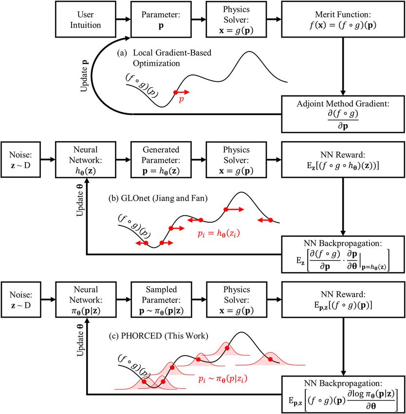
3846 | S. Hooten et al.: Inverse design of grating couplers with PHORCED

With a dense search, the global optimum along the domain Using information from the merit function values, the neu-
of interest can potentially be found. ral network learns to update the mean and standard devia-
 Our technique, called PHORCED, is provided in tion of the Gaussians. Consequently, we emphasize that the
Figure 1(c). Qualitatively speaking, it is very similar to Gaussian policy distribution is not static because its statis-
GLOnet, but is motivated differently from a mathematical tical parameters are adjusted by the trainable weights of
perspective. PHORCED is a special case of the REINFORCE the neural network, and is therefore capable of exploring
algorithm [61, 62] from the field of reinforcement learn- throughout the feasible design space. For adequate choice
ing (RL), applied to electromagnetic inverse design. In of distribution and dense enough search, the PHORCED
particular, the neural network is treated as purely prob- method can potentially find the global optimum in the
abilistic, defining a continuous conditional probability domain of interest.
density function over parameter variables p conditioned Before proceeding it should be remarked that the algo-
on the input vector z – denoted by (p|z). In other words, rithms implemented by GLOnet and PHORCED have prece-
instead of outputting p deterministically given input noise, dent in the literature, with some distinctions that we will
the neural network outputs probabilities of generating p. outline here. Optimization algorithms similar to GLOnet
We then randomly sample a parameter vector p for simu- were suggested in Refs. [64, 65], where the main algo-
lation and evaluation of the reward. Note that (p|z) is rithmic difference appears in the definition of the reward
called the policy in RL, and in this work is chosen to be a function. In particular, the reward defined in Ref. [64]
multivariate Gaussian distribution with mean vector and was the same generalized form that we have presented
standard deviation of random variable p as outputs. The in Figure 1(b), while Jiang and Fan emphasized the use of
reward for PHORCED is qualitatively the same as GLOnet an exponentially-weighted reward to enhance global opti-
– namely, we intend to optimize the expected value of the mization efforts [25]. On the other hand, PHORCED was
electromagnetic merit function. However, because both p motivated as a special case of the REINFORCE algorithm
and z are random variables, we take the joint expected [61, 62], but also resembles some versions of evolutionary
value: p,z [( f ⚬ g)(p)]. Furthermore, because of the proba- strategy [64–67]. The main difference between PHORCED
bilistic representation of the neural network, the gradient and evolutionary strategy (ignoring several heuristics) is
of the reward with respect to the neural net weights for the explicit use of a neural network to model the mul-
backpropagation is much different than the corresponding tivariate Gaussian policy distribution, albeit some recent
GLOnet case. In particular, we find that the backpropa- works have used neural networks in their implementa-
gated chain-rule gradient requires no evaluation of the tions of evolutionary strategy [65, 67] for different appli-
gradient of the electromagnetic merit function, ( f p⚬ g) . cations than those studied here. Furthermore, PHORCED
Consequently, the electromagnetic adjoint simulation is does not require a Gaussian policy; any explicitly-defined
no longer required, implying that fewer simulations are probability distribution can be used as an alternative if
required overall for PHORCED compared to GLOnet under desired. Beyond evolutionary strategy, a recent work in
equivalent choices of neural network architecture and fluid dynamics [68] uses an algorithm akin to PHORCED
hyperparameters.2 PHORCED is visually illustrated in the called One-Step Proximal Policy Optimization (PPO-1) – a
center of Figure 1(c). The neural network defines Gaussian version of REINFORCE with a single policy, , operat-
probability density functions conditioned on input noise ing on parallel instances of the optimization problem. The
vectors zi , shown in the light red bell curves represent- main distinction between PPO-1 and PHORCED is that we
ing (p|zi ), from which we sample points pi to simulate.3 have implemented the option to use an input noise vec-
 tor z to condition the output policy distribution, (x|z),
 which can effectively instantiate multiple distinct policies
 acting on parallel instances of the optimization problem.
2 However, because the representation of the neural network is dif- This potentially enables multi-modal exploration of the
ferent in either case, it would rarely make sense to use equivalent parameter space, bypassing a known issue of Bayesian
choices of neural network architecture and hyperparameters. There- optimization with Gaussian probability distributions [65].
fore, we make this claim tepidly, emphasizing only that we do not
 However, note that the best results for the applications
require adjoint simulations in the evaluation of the reward.
 studied in this work used a constant input vector z, thus
3 Note that while we explored a uniform distribution at the input
as well, our best results with PHORCED applied to grating coupler
optimization in this work were attained with z drawn from a Dirac
delta distribution, i.e. a constant vector input rather than noise. This Figure 1(c) into a single distribution from which we draw multiple
has the effect of collapsing the multiple distributions depicted in samples.

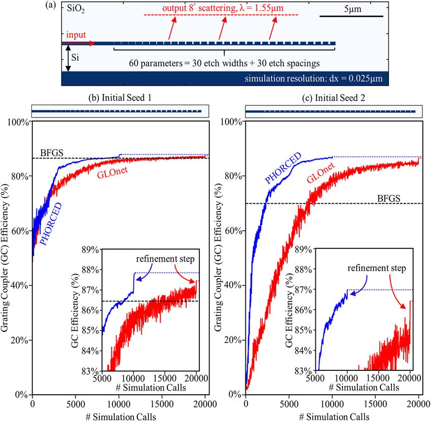
S. Hooten et al.: Inverse design of grating couplers with PHORCED | 3847

making our implementation similar to PPO-1 in the results include fabrication constraints nor other specifications of
below. Regardless of the intricacies mentioned above, we interest in grating couplers in our parameterization choice,
emphasize that both GLOnet and PHORCED are unique in e.g. the BOX thickness and the Si etch depth, which will be
their application to electromagnetic optimization, to the desirable in future optimizations of experimentally-viable
authors’ knowledge. In the next section we will compare devices. Furthermore, the simulation domain is discretized
all three algorithms from Figure 1 applied to grating coupler with a dx = 25 nm grid step which may result in some
optimization. inaccuracy for very fine grating coupler features. This sim-
 ulation discretization was chosen for feasibility of the
 optimization since individual simulations require about
3 Proof-of-concept grating coupler 4 s to compute on a high-performance server with over 30
 concurrent MPI processes, and as we will show GLOnet
 optimization
 and PHORCED can require as many as 20,000 simulation
 evaluations for convergence. Nevertheless, we utilized per-
A grating coupler is a passive photonic device that is
capable of efficiently diffracting light from an on-chip mittivity smoothing [43] to minimize the severity of this
waveguide to an external optical fiber. Recent works have effect and obtain physically meaningful results.
leveraged inverse design techniques in the engineering We apply the Broyden–Fletcher–Goldfarb–Shanno
of grating couplers, resulting in state-of-the-art charac- (BFGS), GLOnet, and PHORCED algorithms to grating cou-
teristics [21, 42, 44, 52, 56]. In this section we will show pler optimization with two different initial designs (Initial
how generative neural networks can aid in the design of Seed 1 and Initial Seed 2) in Figure 2(b) and (c). Initial
ultra-efficient grating couplers. Seed 1 corresponds to the grating depicted in Figure 2(a)
 The grating coupler geometry used for our proof-of- and the top of Figure 2(b), where we used a parameter
concept is depicted in Figure 2(a). We assume a silicon- sweep to choose a linear apodization of the etch duty cycle
on-insulator (SOI) wafer platform with a 280 nm-thick before optimization. Initial Seed 2 corresponds to the grat-
silicon waveguide separated from the silicon substrate ing shown at the top of Figure 2(c) where we use a uniform
by a 2 μm buried oxide (BOX) layer. The grating coupler duty cycle of 90%. Both initial designs have pitch that sat-
consists of periodically spaced corrugations to the input isfy the grating equation [44, 52] for 8◦ scattering. These
silicon waveguide with etch depth 190 nm. These grating initial seeds serve to explore the robustness of the opti-
coupler dimensions are characteristic of a high-efficiency mization algorithms to “good” and “poor” choices of initial
integrated photonics platform operating in the C-band condition. Indeed, Initial Seed 1 satisfies physical intuition
(1550 nm central wavelength) as suggested by a transfer for a good grating coupler, because chirping the duty cycle
matrix based directionality calculation [55, 69], and are is well-known to improve Gaussian beam mode-matching,
provided as an example in the open-source electromag- and thus the initial grating coupler efficiency is already
netic optimization package EMopt [63] that was used to
 a reasonable value of 56%. Meanwhile, Initial Seed 2 has
perform forward and adjoint simulations in this work.
 the correct pitch for 8◦ scattering, but has a low efficiency
 For our optimizations, we will consider 60 total des-
 of 1% owing to poor mode-matching and directionality. In
ignable parameters that define the grating coupler: the
 essence, we are using these two cases as a proxy to explore
width of and spacing between 30 waveguide corrugations.
 whether PHORCED and GLOnet can reliably boost electro-
For a well-designed grating coupler, input light to the
 magnetic performance in a high-dimensional parameter
waveguide scatters at some angle relative to vertical toward
 space, even in cases where the intuition about the optimal
an external optical fiber. In this work we choose to opti-
mize the grating coupler at fixed wavelength and scatter- initial conditions is limited.
ing angle assuming specific manufacturing and assembly BFGS is a conventional gradient-based optimization
requirements for a modular optical transceiver application algorithm similar to that depicted in Figure 1(a), and imple-
[52, 70]. In our case, the merit function for optimization is mented using default settings from the open-source SciPy
the coupling efficiency of scattered light with wavelength optimize module. After optimization with BFGS, the final
 = 1550 nm propagating 8◦ relative to normal, mode- simulated grating coupler efficiency of Initial Seed 1 and
matched to an output Gaussian beam mode field diameter Initial Seed 2 are 86.4 and 69.9% respectively, which are
10.4 μm – characteristic of a typical optical fiber mode. shown in the black dashed lines of Figure 2(b) and (c).
The explicit definition of this electromagnetic merit func- Note that the number of simulation calls for BFGS is not
tion may be found in Refs. [44, 52, 71]. Note that we did not shown because it is vastly smaller than that required for

3848 | S. Hooten et al.: Inverse design of grating couplers with PHORCED

Figure 2: PHORCED and GLOnet outperform conventional gradient-based optimization, with different simulation evaluation requirements.
The grating coupler simulation geometry for optimization is shown in (a), consisting of an SOI wafer platform with 280 nm waveguide,
190 nm etch depth, and 2 μm BOX height. We optimized 60 device parameters in total, namely the width and spacing between 30 etch
corrugations. The results of the BFGS, GLOnet, and PHORCED algorithms applied to Initial Seed 1 and Initial Seed 2 are presented in (b) and
(c) as a function of the number of simulation calls. The initial seeds (grating designs) are illustrated above each optimization plot. The insets
depict zoomed-in views of the peak efficiencies attained by PHORCED and GLOnet, along with respective BFGS refinement steps performed
on the best design generated by each algorithm.

GLOnet and PHORCED (144 and 214 total simulations for [24, 25] with a chosen hyperparameter = 0.6. PHORCED
Initial Seed 1 and Initial Seed 2, respectively). is described qualitatively in Figure 1(c) where we use
 The implementation of GLOnet and PHORCED for the a probabilistic neural network modeling a multivari-
grating coupler optimizations in Figure 2(b) and (c) are ate, isotropic Gaussian output distribution. The electro-
described below; other details and specifications, such magnetic merit function used in the reward is just the
as a graphical illustration of the neural network mod- unweighted grating coupler efficiency, except we used a
els used in either case, may be found in Supplementary “baseline” subtraction of the average merit function value
Materials Section 2. GLOnet is described qualitatively in the backpropagated gradient (which is a common tac-
in Figure 1(b) where we use a deterministic neural tic in reinforcement learning for reducing model variance
network and an exponentially-weighted electromagnetic [72]). In both methods, we use a stopping criterion of 1000
merit function originally recommended by Jiang and Fan total optimizer iterations, with 10 devices sampled per

S. Hooten et al.: Inverse design of grating couplers with PHORCED | 3849

iteration. Note that because GLOnet requires an adjoint GLOnet, respectively. Since PHORCED and GLOnet are
simulation for each device and PHORCED does not, the inherently statistical and noisy, the refinement step is use-
effective stopping criteria are 1000 × 10 × 2 = 20, 000 sim- ful for finding the nearest optimum without requiring one
ulation calls for GLOnet and 1000 × 10 × 1 = 10, 000 sim- to run an exhaustive search of the neural network generator
ulation calls for PHORCED. The neural network models for in inference mode.
GLOnet and PHORCED were implemented in PyTorch, and In summary, we find that the PHORCED + BFGS refine-
are illustrated in Figure S1 of the Supplementary Material. ment optimization achieved the best performance for both
For GLOnet, we used a convolutional neural network with Initial Seed 1 and Initial Seed 2 with final grating coupler
ReLU activations and linear output of the design vector. efficiency of 87.8 and 87.0%, respectively. These results
For PHORCED, we used a simple fully-connected neural agree with a transfer matrix based directionality analysis
network with ReLU activations and linear output defin- of these grating coupler dimensions [55, 69], where we
ing the statistical parameters (mean and variance) of find that approximately 88% grating efficiency is possi-
the Gaussian policy distribution. We applied initial con- ble under perfect mode-matching conditions – meaning
ditions by adding the design vector representing Initial that our result for Initial Seed 1 is close to a theoretical
Seed 1 and Initial Seed 2 to either the direct neural net- global optimum. Notably, GLOnet had better performance
work output or the mean of the Gaussian distribution than PHORCED in Initial Seed 1 before the refinement step
for GLOnet and PHORCED, respectively. Hyperparame- was applied, and it is possible that better results could
ters such as the number of weights and learning rate of have been achieved with further iterations of both algo-
the neural network optimizer were individually tuned for rithms (as indicated by the slowly rising slopes of the
GLOnet and PHORCED (specifications can be found in optimization curves in the insets of Figure 2(b) and (c)).
Figure S2 of the Supplemental Material). For both neu- However, we emphasize that PHORCED required approx-
ral networks, we used an input vector z of dimension 5. imately 2× fewer simulation than GLOnet with the same
However, for GLOnet z was drawn from a uniform distribu- number of optimization iterations because of the lack of
tion  (−1, 1), while for PHORCED we used a simple Dirac adjoint gradient calculations.
delta distribution centered on 1. In other words, the input Perhaps the most important result of these optimiza-
for PHORCED was a constant vector of 1’s. In this work tions is that both PHORCED and GLOnet proved to be
we achieved our best results with this choice, but simi- resilient against our choice of initial condition. Indeed,
lar results (within 1% absolute grating coupler efficiency) while BFGS provided a competitive result for Initial Seed
could be attained with alternative choices of input distribu- 1, it failed to find a favorable local optimum given Initial
tion. Anecdotally, we found that using a noisy input could Seed 2. PHORCED and GLOnet, on the other hand, attained
improve training stability and performance in toy prob- final results within 1% absolute grating coupler efficiency
lems studied outside of this work, but further investigation for both initial conditions. This outcome is promising when
is required. considering the relative sparsity of each algorithm’s search
 We find that PHORCED and GLOnet outperform regu- in a high-dimensional design space. Indeed, as mentioned
lar BFGS for both initial conditions studied in Figure 2. For previously, we only sampled 10 devices per iteration of
Initial Seed 1 (Figure 2(b)), we generated optimized grat- the optimization, meaning that there were fewer samples
ing coupler efficiencies of 86.9 and 87.2% for PHORCED than dimension of the resulting parameter vectors (60). As
and GLOnet, respectively. For Initial Seed 2 (Figure 2(c)) an additional reference, we compared our results to CMA-
we find optimized grating coupler efficiencies of 86.8 and ES (implemented with the open-source package pycma),
85.6% for PHORCED and GLOnet, respectively. Further- a popular “blackbox” global optimization algorithm that
more, as shown in the insets of Figure 2(b) and (c), we is known to be effective for high-dimensional optimiza-
were able to marginally improve each of the results by tion [66]. Under the same number of simulation calls as
applying a BFGS “refinement step” to the best performing PHORCED (10,000), CMA-ES reached efficiencies of 87.3
design output from GLOnet and PHORCED. This refine- and 86.7% for Initial Seed 1 and Initial Seed 2, respectively.
ment step was limited to a maximum of 200 iterations, Therefore our implementations of PHORCED and GLOnet
or until another default convergence criterion was met. are competitive with current state-of-the-art blackbox algo-
For Initial Seed 1 we obtained improvements of {86.9% rithms. While the simulation requirements for convergence
→ 87.8%}/{87.2% → 87.4%} for PHORCED/GLOnet, res- of PHORCED and GLOnet remain computationally pro-
pectively. For Initial Seed 2, we find improvements hibitive for more complex electromagnetic structures than
of {86.8% → 87.0%}/{85.6% → 86.4%} for PHORCED/ those studied here, in contrast to local gradient-based

3850 | S. Hooten et al.: Inverse design of grating couplers with PHORCED

search, our results offer the possibility of global optimiza- PHORCED for the design of 8◦ grating couplers can be
tion effort in electromagnetic design problems, where we retrained to design grating couplers with varied scattering
are capable of limiting the tradeoff of performance with angle and increased rate of convergence.
search density as well as the need for human interven- Transfer learning applied to grating coupler optimiza-
tion in situations where physical intuition is more difficult tion is qualitatively illustrated in Figure 3(a) and (b).
to ascertain. Furthermore, we believe that our implemen- Figure 3(a) shows a shorthand version of the PHORCED
tations of GLOnet and PHORCED have significant room optimization of Initial Seed 1 that was performed in
for improvement, and have advantages that go beyond Figure 2(b), where a neural network was specifically
alternative global optimization algorithms like CMA-ES. In trained to design an 8◦ grating coupler. In the case of
particular, leveraging advanced concepts in deep learning transfer learning in Figure 3(b), we reuse the trained neu-
and reinforcement learning can further improve computa- ral network from Figure 3(a) but now exchange the 8◦
tional efficiency and performance. For example, whereas angle in the grating coupler efficiency merit function with
our implementations of PHORCED and GLOnet used sim- an alternate scattering angle. In particular, we retrain the
ple neural networks, a ResNet architecture can improve neural network on six alternative grating coupler angles:
neural network generalizability while simultaneously red- {2◦ , 4◦ , 6◦ , 10◦ , 12◦ , 14◦ }. Note that we maintained the exact
ucing overfitting [27]. Moreover, one could take advan- same neural network architecture and optimization hyper-
tage of complementary deep learning and reinforcement parameters during these exchanges, including the opti-
learning based approaches such as importance sampling mization stopping criterion of 10,000 total simulation calls
[65, 72], or “model-based” methods that could utilize per training session; the only change in a given opti-
an electromagnetic surrogate model or inverse model to mization was the grating coupler angle. As depicted in
reduce the number of full electromagnetic Maxwell sim- Figure 3(c), we show the optimization progressions of these
ulations needed for training [13, 19, 28, 32]. Alternatively, transfer learning sessions (blue/red curves) in comparison
whereas we optimized our grating for a single objective to the original PHORCED optimization of the 8◦ grating
(single wavelength, 8◦ scattering) Jiang and Fan showed coupler from Figure 2(b) (reproduced in the black curve
that generative neural network based optimization can in the middle panel). Also shown are control optimiza-
be extremely efficient for multi-objective design problems tions for each grating coupler angle using the PHORCED
(e.g., multiple wavelengths and scattering angles in meta- method without transfer learning (in gray). We find that
surfaces [24]). Along the same vein, in the next section transfer learning to grating couplers with nearby scatter-
we will show how a technique known as transfer learn- ing angles (e.g. 6◦ and 10◦ ) exhibit extremely accelerated
ing can be used to repurpose a neural network trained rate of convergence relative to the original optimization
with PHORCED for an alternative objective, meanwhile and control cases. However, transfer learning is less effec-
boosting computational efficiency and electromagnetic tive or ineffective for more distant angles (e.g. 2◦ , 4◦ , and
performance dramatically. 14◦ ). This observation is shown more clearly in Figure 3(d)
 where we plot the number of simulations required to reach
 80% efficiency in optimization versus the scattering angle
4 Transfer learning with the for retraining.4 While the original optimization and control
 PHORCED method optimizations (black star and gray diamonds) required sev-
 eral thousand simulation calls before reaching this thresh-
Transfer learning is a concept in machine learning encom- old, the 6◦ and 10◦ transfer learning optimizations required
passing any method that reuses a model (e.g. a neural only about 100 simulations a piece – a >10× reduction
network) trained on one task for a different but related in simulation calls, making transfer learning comparable
task. Qualitatively speaking and verified by real-world with local gradient-based optimization in terms of compu-
applications, we might expect the retraining of a neural tation requirements. On the other hand, the distant grating
network to occur faster than training a new model from coupler angle transfer learning optimizations (2◦ , 4◦ , and
scratch. Transfer learning has been extensively applied 14◦ ) required similar simulation call requirements to reach
in classical machine learning tasks such as classification the same threshold as the original optimization. Evidently,
and regression, but has only recently been mentioned in
the optics/photonics research domains [17, 27, 28, 33]. In
this work we apply transfer learning to the inverse design 4 80% grating coupler efficiency was chosen because it equates to
of integrated photonics for the first time (to the authors’ roughly 1 dB insertion loss – an optimistic target for state-of-the-art
knowledge), revealing that a neural network trained using silicon photonic devices.

S. Hooten et al.: Inverse design of grating couplers with PHORCED | 3851

Figure 3: Transfer learning applied to grating coupler design yields accelerated convergence rate in optimization. The original PHORCED
optimization from Figure 2(b) is qualitatively depicted as a block diagram in (a) for comparison with the transfer learning approach in (b).
Here, we exchange the 8◦ grating coupler merit function with an alternative grating coupler angle for retraining. Optimization progressions
as a function of the number of simulation calls for each of the retraining sessions are shown in the blue/red curves of (c). Control
optimizations where transfer learning was not applied are plotted in gray for comparison. In (d) we plot the number of simulation calls for
each optimization from (c) to reach 80% grating coupler scattering efficiency, with blue/red colored arrows and dots indicating applications
of transfer learning and gray diamonds indicating the control cases.

there is a bias towards less effective transfer learning for advantage for optimizations at more distant grating
small scattering angles. Grating couplers become plagued coupler angles? We explore this question of sequential
by parasitic back-reflection for small diffraction angles transfer learning in Figure 4. In Figure 4(a) and (b) we
relative to normal [44, 52], and thus it is possible that the qualitatively compare sequential transfer learning to the
neural network has difficulty adapting to the new physics original PHORCED optimization from Figure 2(b). As indi-
that were not previously encountered. We conclude that cated, we replace the original 8◦ grating coupler scat-
the transfer learning approach is most effective for devices tering angle in the electromagnetic merit function with
with very similar physics to the device originally optimized an alternative scattering angle in the same manner dis-
by the neural network. cussed in Figure 3(b). Then, after that optimization has
 The results of Figure 3 lead to a natural follow- completed, we continue to iterate and exchange the grat-
up query: can we apply transfer learning multiple times ing coupler angle again. By sequentially applying trans-
progressively in order to maintain the convergence rate fer learning, we hope to slowly introduce new physics

3852 | S. Hooten et al.: Inverse design of grating couplers with PHORCED

Figure 4: Transfer learning applied sequentially improves convergence for grating coupler scattering angles that are distant relative to the
original optimization’s scattering angle. The original PHORCED optimization from Figure 2(b) is qualitatively depicted in (a) for comparison
with the ‘‘sequential’’ transfer learning approach in (b). Here, we sequentially re-train the neural network (originally trained to generate 8◦
grating couplers) with progressively different scattering angles, with the intention of slowly changing the physics seen by the neural
network. Grating coupler efficiency as a function of the number of simulation calls for each of the retraining sessions are shown in the
blue/red curves of (c), where the arrows on the right-hand side show the sequence of each application of transfer learning. The results of the
one-shot (non-sequential) transfer learning approach from Figure 3(c) are shown in gray for comparison. In (d) we plot the number of
simulation calls needed for the grating coupler optimizations from (c) to reach an 80% efficiency using the sequential transfer learning
approach, similar to the corresponding plot in Figure 3(d). The blue/red arrows and dots indicate applications of sequential transfer
learning, and the gray diamonds correspond to non-sequential transfer learning cases.

to the neural network such that we can maintain faster the same as those shown previously in Figure 3(c); the
convergence at more physically distant problems from the new results may be seen in the 2◦ , 4◦ , 12◦ , and 14◦ cases,
initial optimization. We conduct two sequential transfer where blue/red lines indicate the new optimization data
learning sessions where we evolve the grating coupler scat- and gray lines indicate the non-sequential transfer learn-
tering angle in the following steps: {8◦ → 10◦ → 12◦ → 14◦ } ing cases from Figure 3(c) for comparison. We observe that
and {8◦ → 6◦ → 4◦ → 2◦ }. The results of these progressions sequential transfer learning improves the optimization
are shown in Figure 4(c) where we plot the grating coupler convergence rate for the distant grating coupler scatter-
efficiency as a function of the number of simulation calls ing angles, in accordance with our initial prediction. This
in each (re-)training session. The 6◦ , 8◦ , and 10◦ cases are observation is made more explicit in Figure 4(d) where

S. Hooten et al.: Inverse design of grating couplers with PHORCED | 3853

we plot the simulation call requirement to reach an 80% gradient-based BFGS optimization, resulting in state-of-
grating coupler efficiency threshold for each of the trans- the-art simulated insertion loss for single-etch c-Si grating
fer learning optimizations. Blue/red arrows and points couplers and resilience against poor choices of initial con-
indicate sequential transfer learning progressions, while dition. In future work we intend to implement fabrication
gray diamonds indicate the one-shot transfer learning constraints, alternative choices of geometrical parame-
cases reproduced from Figure 3(d). Evidently, sequential terization, and other criteria to guarantee feasibility and
transfer learning improves simulation call requirements robustness of experimental devices.
by approximately an order of magnitude relative to the As an additional contribution we introduced the con-
single-step cases. While we find that there is still a notice- cept of transfer learning to integrated photonic opti-
able bias towards longer (but less severely long) training mization, revealing that a trained neural network using
at smaller scattering angles, sequential transfer learn- PHORCED could be re-trained on alternative problems with
ing had the added benefit of providing the most efficient accelerated convergence. In particular, we showed that
devices overall at every scattering angle in the progres- transfer learning could be applied to the design of grat-
sion. Note that the plotted simulation call requirements do ing couplers with varied scattering angle. Transfer learn-
not include the simulation calls from the previous itera- ing was extremely effective for grating coupler scattering
tion in the sequential transfer learning progression (each angles within ≈ ±4◦ to the original optimization angle,
application of transfer learning used 10,000 simulation improving the convergence rate by >10× in some cases.
calls, where the final neural network weightset after those However, this range could be effectively extended to ≈ ±6◦
10,000 simulation calls was used as the initial weightset or more using a sequential transfer learning approach,
for the next iteration of transfer learning). Furthermore, where transfer learning was applied multiple times pro-
note that each optimization in these sequential transfer gressively to slowly change the angle seen by the neural
learning cases used the same neural network architecture network. Because neural network based design methods
and hyperparameters as the original PHORCED optimiza- such as PHORCED are generally data-hungry, we believe
tion (8◦ case), except for the {12◦ → 14◦ } and {4◦ → 2◦ } that transfer learning could greatly reduce the electromag-
cases which required a slightly smaller learning rate in netic simulation and compute time that would otherwise
optimization for better performance. The smaller learning be required by these techniques in the design of complex
rate negligibly affected the 80% efficiency simulation call electromagnetic structures. For example, transfer learning
requirement shown in Figure 4(d). could be used in multiple hierarchical stages to evolve an
 optimization from a two-dimensional structure to a three-
 dimensional structure, or from a surrogate model (e.g., the
5 Conclusions grating coupler model in Ref. [10]) to real physics.
 Looking forward, we would like to emphasize that
In this work we introduced PHORCED, a photonic optimiza- PHORCED takes advantage of fundamental concepts in
tion package leveraging the policy gradient method from reinforcement learning, but there is a plethora of burgeon-
reinforcement learning. This method interfaces a proba- ing contemporary research in this field, such as advanced
bilistic neural network with an electromagnetic solver for policy gradient, off-policy, and model-based approaches.
enhanced inverse design capabilities. PHORCED does not We anticipate that further cross-pollination of the inverse
require an evaluation of adjoint method gradient of the electromagnetic design and reinforcement learning com-
electromagnetic merit function with respect to the design munities could open the floodgates for new research in
parameters, therefore eliminating the need to perform electromagnetic optimization.
adjoint simulations over the course of an optimization. We
anticipate that this fact can be particularly advantageous Acknowledgment: The authors thank S. K. Vadlamani for
for multifrequency electromagnetic merit functions, where reinforcement learning discussions.
multiple adjoint simulations would normally be required in Author contribution: All the authors have accepted respon-
a simple frequency-domain implementation of the adjoint sibility for the entire content of this submitted manuscript
method (e.g. see Ref. [52]). and approved submission.
 We applied both PHORCED and the GLOnet method to Research funding: Hewlett Packard Enterprise.
the proof-of-concept optimization of grating couplers. We Conflict of interest statement: The authors declare no
found that both algorithms could outperform conventional conflicts of interest regarding this article.

3854 | S. Hooten et al.: Inverse design of grating couplers with PHORCED

 neural networks,’’ ACS Photonics, vol. 6, no. 5, pp. 1168 − 1174,
References 2019..
 [18] D. Melati, Y. Grinberg, M. Kamandar Dezfouli, et al., ‘‘Mapping
 [1] Y. Shen, N. C. Harris, S. Skirlo, et al., ‘‘Deep learning with
 the global design space of nanophotonic components using
 coherent nanophotonic circuits,’’ Nat. Photonics, vol. 11,
 machine learning pattern recognition,’’ Nat. Commun., vol. 10,
 pp. 441 − 446, 2016..
 no. 1, pp. 1 − 9, 2019..
 [2] T. Inagaki, Y. Haribara, K. Igarashi, et al., ‘‘A coherent Ising
 [19] M. H. Tahersima, K. Kojima, T. Koike-Akino, et al., ‘‘Deep
 machine for 2000-node optimization problems,’’ Science,
 neural network inverse design of integrated photonic power
 vol. 354, no. 6312, pp. 603 − 606, 2016..
 splitters,’’ Sci. Rep., vol. 9, no. 1, p. 1368, 2019..
 [3] N. C. Harris, G. R. Steinbrecher, M. Prabhu, et al., ‘‘Quantum [20] A. Demeter-Finzi and S. Ruschin, ‘‘S-matrix absolute
 transport simulations in a programmable nanophotonic optimization method for a perfect vertical waveguide grating
 processor,’’ Nat. Photonics, vol. 11, no. 7, pp. 447 − 452, 2017.. coupler,’’ Opt. Express, vol. 27, no. 12, pp. 16713 − 16718,
 [4] Y. Yamamoto, K. Aihara, T. Leleu, et al., ‘‘Coherent Ising 2019..
 machines − optical neural networks operating at the quantum [21] M. K. Dezfouli, Y. Grinberg, D. Melati, et al., ‘‘Design of fully
 limit,’’ npj Quantum Inf., vol. 3, no. 1, pp. 1 − 15, 2017.. apodized and perfectly vertical surface grating couplers using
 [5] E. Khoram, A. Chen, D. Liu, et al., ‘‘Nanophotonic media for machine learning optimization,’’ in Proc. SPIE, Integrated
 artificial neural inference,’’ Photon. Res., vol. 7, no. 8, Optics: Devices, Materials, and Technologies XXV, vol. 11689,
 pp. 823 − 827, 2019.. San Francisco, USA, International Society for Optics and
 [6] T. W. Hughes, I. A. D. Williamson, M. Minkov, and S. Fan, Photonics, 2021, p. 116890J.
 ‘‘Wave physics as an analog recurrent neural network,’’ Sci. [22] M. M. R. Elsawy, S. Lanteri, R. Duvigneau, G. Briére, M. S.
 Adv., vol. 5, no. 12, pp. 1 − 6, 2019.. Mohamed, and P. Genevet, ‘‘Global optimization of
 [7] B. J. Shastri, A. N. Tait, T. Ferreira de Lima, et al., ‘‘Photonics for metasurface designs using statistical learning methods,’’ Sci.
 artificial intelligence and neuromorphic computing,’’ Nat. Rep., vol. 9, no. 1, p. 17918, 2019..
 Photonics, vol. 15, no. 2, pp. 102 − 114, 2021.. [23] A. M. Hammond and R. M. Camacho, ‘‘Designing integrated
 [8] X. Xu, M. Tan, B. Corcoran, et al., ‘‘11 TOPS photonic photonic devices using artificial neural networks,’’ Opt.
 convolutional accelerator for optical neural networks,’’ Nature, Express, vol. 27, no. 21, pp. 29620 − 29638, 2019..
 vol. 589, no. 7840, pp. 44 − 51, 2021.. [24] J. Jiang and J. A. Fan, ‘‘Global optimization of dielectric
 [9] M. Raissi, P. Perdikaris, and G. E. Karniadakis, ‘‘Physics metasurfaces using a physics-driven neural network,’’ Nano
 informed neural networks: a deep learning framework for Lett., vol. 19, no. 8, pp. 5366 − 5372, 2019..
 solving forward and inverse problems involving nonlinear [25] J. Jiang and J. A. Fan, ‘‘Simulator-based training of generative
 partial differential equations,’’ J. Comput. Phys., vol. 378, neural networks for the inverse design of metasurfaces,’’
 pp. 686 − 707, 2019.. Nanophotonics, vol. 9, no. 5, pp. 1059 − 1069, 2020..
[10] D. Gostimirovic and W. N. Ye, ‘‘An open-source artificial neural [26] J. Jiang and J. A. Fan, ‘‘Multiobjective and categorical global
 network model for polarization-insensitive silicon-on-insulator optimization of photonic structures based on ResNet
 subwavelength grating couplers,’’ IEEE J. Sel. Top. Quant. generative neural networks,’’ Nanophotonics, vol. 10, no. 1,
 Electron., vol. 25, no. 3, pp. 1 − 5, 2019.. pp. 361 − 369, 2020..
 [11] Y. Guo, X. Cao, B. Liu, and M. Gao, ‘‘Solving partial differential [27] J. Jiang, M. Chen, and J. A. Fan, ‘‘Deep neural networks for the
 equations using deep learning and physical constraints,’’ evaluation and design of photonic devices,’’ Nat. Rev. Mater.,
 Appl. Sci., vol. 10, no. 17, p. 5917, 2020.. vol. 6, no. 8, pp. 679 − 700, 2021..
[12] Y. Chen, L. Lu, G. E. Karniadakis, and L. D. Negro, [28] R. S. Hegde, ‘‘Deep learning: a new tool for photonic
 ‘‘Physics-informed neural networks for inverse problems in nanostructure design,’’ Nanoscale Adv., vol. 2, no. 3,
 nano-optics and metamaterials,’’ Opt. Express, vol. 28, no. 8, pp. 1007 − 1023, 2020..
 pp. 11618 − 11633, 2020.. [29] M. Minkov, I. A. Williamson, L. C. Andreani, et al., ‘‘Inverse
[13] R. Pestourie, Y. Mroueh, T. V. Nguyen, P. Das, and S. G. design of photonic crystals through automatic differentiation,’’
 Johnson, ‘‘Active learning of deep surrogates for PDEs: ACS Photonics, vol. 7, no. 7, pp. 1729 − 1741, 2020..
 application to metasurface design,’’ npj Comput. Mater., [30] S. So, T. Badloe, J. Noh, J. Rho, and J. Bravo-Abad, ‘‘Deep
 vol. 6, no. 1, pp. 1 − 7, 2020.. learning enabled inverse design in nanophotonics,’’
[14] A. Ghosh, D. J. Roth, L. H. Nicholls, W. P. Wardley, A. V. Zayats, Nanophotonics, vol. 2234, pp. 1 − 17, 2020..
 and V. A. Podolskiy, ‘‘Machine learning-based diffractive [31] Z. Ma and Y. Li, ‘‘Parameter extraction and inverse design of
 image analysis with subwavelength resolution,’’ ACS semiconductor lasers based on the deep learning and particle
 Photonics, vol. 8, no. 5, pp. 1448 − 1456, 2021.. swarm optimization method,’’ Opt. Express, vol. 28, no. 15,
[15] L. Lu, R. Pestourie, W. Yao, Z. Wang, F. Verdugo, and S. G. p. 21971, 2020..
 Johnson, ‘‘Physics-informed neural networks with hard [32] K. Kojima, M. H. Tahersima, T. Koike-Akino, et al., ‘‘Deep
 constraints for inverse design,’’ arXiv:2102.04626 [physics], neural networks for inverse design of nanophotonic devices,’’
 2021. J. Lightwave Technol., vol. 39, no. 4, pp. 1010 − 1019, 2021..
[16] R. Trivedi, L. Su, J. Lu, M. F. Schubert, and J. Vuckovic, [33] W. Ma, Z. Liu, Z. A. Kudyshev, A. Boltasseva, W. Cai, and Y. Liu,
 ‘‘Data-driven acceleration of photonic simulations,’’ Sci. Rep., ‘‘Deep learning for the design of photonic structures,’’ Nat.
 vol. 9, no. 1, pp. 1 − 7, 2019.. Photonics, vol. 15, no. 2, pp. 77 − 90, 2021..
[17] Y. Qu, L. Jing, Y. Shen, M. Qiu, and M. Soljačić, ‘‘Migrating [34] D. Melati, M. Kamandar Dezfouli, Y. Grinberg, et al., ‘‘Design of
 knowledge between physical scenarios based on artificial compact and efficient silicon photonic micro antennas with

S. Hooten et al.: Inverse design of grating couplers with PHORCED | 3855

 perfectly vertical emission,’’ IEEE J. Sel. Top. Quant. Electron., [51] E. Bayati, R. Pestourie, S. Colburn, Z. Lin, S. G. Johnson, and A.
 vol. 27, no. 1, pp. 1 − 10, 2021.. Majumdar, ‘‘Inverse designed metalenses with extended depth
[35] R. Hegde, ‘‘Sample-efficient deep learning for accelerating of focus,’’ ACS Photonics, vol. 7, no. 4, pp. 873 − 878, 2020..
 photonic inverse design,’’ OSA Continuum, vol. 4, no. 3, [52] S. Hooten, T. V. Vaerenbergh, P. Sun, S. Mathai, Z. Huang, and
 pp. 1019 − 1033, 2021.. R. G. Beausoleil, ‘‘Adjoint optimization of efficient
[36] J. S. Jensen and O. Sigmund, ‘‘Topology optimization for CMOS-compatible Si-SiN vertical grating couplers for DWDM
 nano-photonics,’’ Laser Photon. Rev., vol. 5, no. 2, applications,’’ J. Lightwave Technol., vol. 38, no. 13,
 pp. 308 − 321, 2011.. pp. 3422 − 3430, 2020..
[37] J. Lu and J. Vučković, ‘‘Objective-first design of high efficiency, [53] W. Jin, S. Molesky, Z. Lin, K. M. C. Fu, and A. W. Rodriguez,
 small-footprint couplers between arbitrary nanophotonic ‘‘Inverse design of compact multimode cavity couplers,’’ Opt.
 waveguide modes,’’ Opt. Express, vol. 20, no. 7, Express, vol. 26, no. 20, pp. 26713 − 26721, 2018..
 pp. 7221 − 7236, 2012.. [54] W. Jin, W. Li, M. Orenstein, and S. Fan, ‘‘Inverse design of
[38] C. M. Lalau-Keraly, S. Bhargava, O. D. Miller, and E. lightweight broadband reflector for relativistic lightsail
 Yablonovitch, ‘‘Adjoint shape optimization applied to propulsion,’’ ACS Photonics, vol. 7, no. 9, pp. 2350 − 2355,
 electromagnetic design,’’ Opt. Express, vol. 21, no. 18, pp. 21, 2020..
 2013.. [55] A. Michaels, M. C. Wu, and E. Yablonovitch, ‘‘Hierarchical
[39] Y. Elesin, B. S. Lazarov, J. S. Jensen, and O. Sigmund, ‘‘Time design and optimization of silicon photonics,’’ IEEE J. Sel. Top.
 domain topology optimization of 3D nanophotonic devices,’’ Quant. Electron., vol. 26, no. 2, pp. 1 − 12, 2020..
 Photonics Nanostructures: Fundam. Appl., vol. 12, no. 1, [56] P. Sun, T. V. Vaerenbergh, M. Fiorentino, and R. Beausoleil,
 pp. 23 − 33, 2014.. ‘‘Adjoint-method-inspired grating couplers for CWDM O-band
[40] A. Y. Piggott, J. Lu, K. G. Lagoudakis, J. Petykiewicz, T. M. applications,’’ Opt. Express, vol. 28, no. 3, pp. 3756 − 3767,
 Babinec, and J. Vučković, ‘‘Inverse design and demonstration 2020..
 of a compact and broadband on-chip wavelength demulti- [57] Z. Lin, C. Roques-Carmes, R. Pestourie, M. Soljačić, A.
 plexer,’’ Nat. Photonics, vol. 9, no. 6, pp. 374 − 377, 2015.. Majumdar, and S. G. Johnson, ‘‘End-to-end nanophotonic
[41] L. F. Frellsen, Y. Ding, O. Sigmund, and L. H. Frandsen, inverse design for imaging and polarimetry,’’ Nanophotonics,
 ‘‘Topology optimized mode multiplexing in silicon-on-insulator vol. 10, no. 3, pp. 1177 − 1187, 2021..
 photonic wire waveguides,’’ Opt. Express, vol. 24, no. 15, [58] Z. Omair, S. M. Hooten, and E. Yablonovitch, ‘‘Broadband
 pp. 16866 − 16873, 2016.. mirrors with >99% reflectivity for ultra-efficient
[42] L. Su, R. Trivedi, N. V. Sapra, A. Y. Piggott, D. Vercruysse, and thermophotovoltaic power conversion,’’ in Proc. SPIE, Energy
 J. Vučković, ‘‘Fully-automated optimization of grating Harvesting and Storage: Materials, Devices, and Applications
 couplers,’’ Opt. Express, vol. 26, no. 4, pp. 2614 − 2617, 2017.. XI, vol. 11722, Orlando, USA, International Society for Optics
[43] A. Michaels and E. Yablonovitch, ‘‘Leveraging continuous and Photonics, 2021, p. 1172208.
 material averaging for inverse electromagnetic design,’’ Opt. [59] D. Vercruysse, N. V. Sapra, K. Y. Yang, and J. Vučković,
 Express, vol. 26, no. 24, pp. 31717 − 31737, 2018.. ‘‘Inverse-designed photonic crystal devices for optical beam
[44] A. Michaels and E. Yablonovitch, ‘‘Inverse design of near unity steering,’’ arXiv:2102.00681 [physics], 2021.
 efficiency perfectly vertical grating couplers,’’ Opt. Express, [60] Z. Zeng, P. K. Venuthurumilli, and X. Xu, ‘‘Inverse design of
 vol. 26, no. 4, pp. 4766 − 4779, 2018.. plasmonic structures with FDTD,’’ ACS Photonics, vol. 8, no. 5,
[45] S. Molesky, Z. Lin, A. Y. Piggott, W. Jin, J. Vucković, and A. W. pp. 1489 − 1496, 2021..
 Rodriguez, ‘‘Inverse design in nanophotonics,’’ Nat. Photonics, [61] R. J. Williams, ‘‘Simple statistical gradient-following
 vol. 12, no. 11, pp. 659 − 670, 2018.. algorithms for connectionist reinforcement learning,’’ Mach.
[46] T. W. Hughes, M. Minkov, I. A. D. Williamson, and S. Fan, Learn., vol. 8, no. 3, pp. 229 − 256, 1992..
 ‘‘Adjoint method and inverse design for nonlinear [62] R. S. Sutton, D. McAllester, S. Singh, and Y. Mansour, ‘‘Policy
 nanophotonic devices,’’ ACS Photonics, vol. 5, no. 12, gradient methods for reinforcement learning with function
 pp. 4781 − 4787, 2018.. approximation,’’ in Advances in Neural Information Processing
[47] Y. Liu, W. Sun, H. Xie, et al., ‘‘Very sharp adiabatic bends Systems, vol. 12, S. Solla, T. Leen, and K. Müller, Eds.,
 based on an inverse design,’’ Opt. Lett., vol. 43, no. 11, Cambridge, USA, MIT Press, 2000.
 pp. 2482 − 2485, 2018.. [63] A. Michaels, EMopt, 2019 [Online]. Available at: https://github
[48] N. M. Andrade, S. Hooten, S. A. Fortuna, K. Han, E. .com/anstmichaels/emopt.
 Yablonovitch, and M. C. Wu, ‘‘Inverse design optimization for [64] L. Faury, F. Vasile, C. Calauzénes, and O. Fercoq, ‘‘Neural
 efficient coupling of an electrically injected optical generative models for global optimization with gradients,’’
 antenna-LED to a single-mode waveguide,’’ Opt. Express, arXiv:1805.08594 [cs], 2018.
 vol. 27, no. 14, pp. 19802 − 19814, 2019.. [65] L. Faury, C. Calauzenes, O. Fercoq, and S. Krichen, ‘‘Improving
[49] D. Vercruysse, N. V. Sapra, L. Su, R. Trivedi, and J. Vučković, evolutionary strategies with generative neural networks,’’
 ‘‘Analytical level set fabrication constraints for inverse arXiv:1901.11271 [cs], 2019.
 design,’’ Sci. Rep., vol. 9, no. 1, pp. 1 − 7, 2019.. [66] N. Hansen, ‘‘The CMA evolution strategy: a tutorial,’’
[50] Y. Augenstein and C. Rockstuhl, ‘‘Inverse design of arXiv:1604.00772 [cs, stat], 2016.
 nanophotonic devices with structural integrity,’’ ACS [67] T. Salimans, J. Ho, X. Chen, S. Sidor, and I. Sutskever,
 Photonics, vol. 7, no. 8, pp. 2190 − 2196, 2020.. ‘‘Evolution strategies as a scalable alternative to
 reinforcement learning,’’ arXiv:1703.03864 [cs, stat], 2017.