Deep action learning enables robust 3D segmentation of body organs in various CT and MRI images - Nature
←
→
Page content transcription
If your browser does not render page correctly, please read the page content below
www.nature.com/scientificreports
OPEN Deep action learning enables
robust 3D segmentation of body
organs in various CT and MRI
images
Xia Zhong1*, Mario Amrehn1, Nishant Ravikumar1, Shuqing Chen1, Norbert Strobel2,
Annette Birkhold3, Markus Kowarschik3, Rebecca Fahrig3 & Andreas Maier1
In this study, we propose a novel point cloud based 3D registration and segmentation framework
using reinforcement learning. An artificial agent, implemented as a distinct actor based on value
networks, is trained to predict the optimal piece-wise linear transformation of a point cloud for the
joint tasks of registration and segmentation. The actor network estimates a set of plausible actions
and the value network aims to select the optimal action for the current observation. Point-wise
features that comprise spatial positions (and surface normal vectors in the case of structured meshes),
and their corresponding image features, are used to encode the observation and represent the
underlying 3D volume. The actor and value networks are applied iteratively to estimate a sequence
of transformations that enable accurate delineation of object boundaries. The proposed approach
was extensively evaluated in both segmentation and registration tasks using a variety of challenging
clinical datasets. Our method has fewer trainable parameters and lower computational complexity
compared to the 3D U-Net, and it is independent of the volume resolution. We show that the
proposed method is applicable to mono- and multi-modal segmentation tasks, achieving significant
improvements over the state-of-the-art for the latter. The flexibility of the proposed framework is
further demonstrated for a multi-modal registration application. As we learn to predict actions rather
than a target, the proposed method is more robust compared to the 3D U-Net when dealing with
previously unseen datasets, acquired using different protocols or modalities. As a result, the proposed
method provides a promising multi-purpose segmentation and registration framework, particular in
the context of image-guided interventions.
Segmentation and registration of anatomical structures in 3D imaging are important pre-processing steps for
clinical applications such as computer aided-diagnosis, treatment planning, or X-ray dose management. Develop-
ing such segmentation and registration method for practical use is challenging, as the method has to be robust
w.r.t. patient anatomy, scan protocols, as well as type, amount, and injection rate of contrast agents. Additionally,
any algorithm, in particular when used in an intra-procedural setting, should involve minimum user interaction
and must have a fast run-time. While many approaches exist treating segmentation and registration as separate
tasks, an approach solving both problems simultaneously as proposed in1 is therefore very appealing. These
methods are usually referred to as model-based or atlas-based segmentation approaches. Employing such a
framework makes it possible to align pre-operatively segmented datasets with intra-operative or post-operative
data, and segment the latter. Despite these advantages, e.g., a good segmentation performance, in particular when
using neural networks, during inference the computational complexity and run-time of such techniques is quite
high. Reducing the inference time in multi-modal segmentation and registration is, however, essential to enable
applications in interventional imaging and endovascular treatment settings, settings such as liver embolization
or transarterial chemo embolization (TRACE). To address this challenge, we introduce a general scheme for joint
point cloud-based joint segmentation and registration based on reinforcement learning.
1
Pattern Recognition Lab, Friedrich-Alexander University, Erlangen‑Nürnberg, Germany. 2Institute of Medical
Engineering, University of Applied Sciences, Würzburg‑Schweinfurt, Germany. 3Siemens Healthcare GmbH,
Forchheim, Germany. *email: xia.zhong@fau.de
Scientific Reports | (2021) 11:3311 | https://doi.org/10.1038/s41598-021-82370-6 1
Vol.:(0123456789)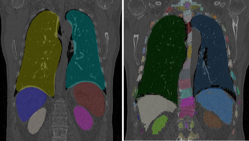
www.nature.com/scientificreports/
3D image segmentation. Image segmentation techniques can be categorized and formulated in different
ways. In this article we categorize the method into model-based (boundary seeking), image-based (voxel-wise
classification) and hybrid methods. Model-based methods deform the current estimate of an object’s bound-
ary to either better conform to a learned appearance, or to obtain an improved alignment with a set of features
designed to represent the structure of interest. This is usually obtained by minimizing a suitable energy func-
tion. Object boundaries may be represented in parametric or non-parametric form. They may be updated: (1)
directly in 3D space using an active shape model (ASM)2, an active appearance model (AAM)3, or a sparse shape
model4; (2) by altering its representation in 4D hyperspace using level-sets5, or (3) by deforming a template, e.g.,
by fitting a probabilistic atlas to the volume of interest6. In image-based methods, each voxel in the volume is
segmented. This group of techniques comprises basic thresholding and Graph-cut7,8. In addition, there is unsu-
pervised clustering9 and artificial neural n etworks10,11. Hybrid methods are a combination of model-based and
image-based approaches12.
With the introduction of convolutional neural networks (CNNs) in recent years, image segmentation
approaches have improved substantially. CNNs have been applied to both image-based and model-based seg-
mentation problems outperforming traditional techniques. With regards to the former, the most noticeable
breakthrough was the introduction of the U-Net for 2D segmentation by Ronneberger et al. 10 Subsequently,
different variations of the U-Net were proposed, which have extended the method to 3 D13,14, dealt with the issue
of class imbalance by adapting the loss function appropriately15, introduced residual b locks16, incorporated
adversarial learning17, or introduced attention mechanisms into the n etwork18. For model-based settings, CNNs
have been used to predict the deformation of a segmented template19, enabling single- and multi-atlas based
segmentation20. Although these methods have shown great success and found widespread adoption in most
medical image segmentation tasks, there are some disadvantages. For example, 3D-CNNs are computationally
expensive with a complexity of O(n3 ) during inference where n denotes the volume size. Although efforts have
been made to accelerate the U-Net for 3D, the segmentation of a volume in its original resolution still needs
about 100s using an NVIDIA Titan X G PU14. Additionally, it is difficult for CNN-based approaches to impose
geometric constraints using a single network. Some recent work uses graph networks21 or CNN for surface
segmentation22 to tackle this problem. Often post-processing steps are necessary to enforce connectivity and to
ensure boundary smoothness. Finally, CNNs are rather sensitive to the dataset. Fine-tuning or transfer learning
is usually required in order to apply a pre-trained CNN to a new dataset, especially when the data is acquired
differently relative to the data used for pre-training23. The difference may, e.g., be due to the use of a different
scan protocol, e.g., a change in tube voltage or a different reconstruction matrix size when using computed
tomography (CT). It could also be caused by use of an entirely different imaging modality, for example, magnetic
resonance tomography (MRT) instead of CT. These factors inhibit the application of conventional CNN-based
segmentation approaches (such as the U-Net) in clinical settings, where different imaging devices from various
vendors set at site-specific acquisition protocols are used.
Parallel to this branch of deep learning approaches, reinforcement learning (RL) has also been investigated
for image analysis. For example Krebs et al.24 used RL to estimate the modes of a 3D deformation field for a vol-
ume. Here, the modes, which are likely to increase the final segmentation accuracy, are iteratively estimated by
the agent. Mo et al. 25 applied RL to train an agent for locating the boundary points of objects in 2D images. The
agent successively identifies and adds boundary locations at each step and, on convergence, the final enclosure
of the trajectory is considered as the segmentation result.
Reinforcement learning in medical image processing. In recent years, there have been significant
improvements in the capabilities of RL-based systems. With the introduction of deep Q-networks (DQN)26
separating policy and value networks27, and actor-critic networks28, RL has shown great success in autonomously
acting in simulated constrained environments, e.g., chess and video games. Furthermore, there is research show-
ing that RL also has great potential in medical image processing, e.g., in anatomical landmark d etection29,30, rigid
image registration31, and non-rigid image r egistration24. A comprehensive review of RL is out of the scope of this
paper, however, we introduce the basic concepts of RL relevant to this work, and adaptation.
Finite Markov decision processes. The fomulation of RL is closely related to the Finite Markov Decision Pro-
cess (MDP). The Finite Markov Decision Process comprises a set of possible states st ∈ St , and a set of possible
actions at ∈ At at time step t. Here, St denotes the set of all possible states, while At refers to the set of all actions.
In addition, for each action at , we have an associated probability πt (at |st ) and an associated immediate reward
rt (at |st ) ∈ Rt with Rt denoting the set of rewards for all possible actions At . At each time step t, the environ-
ment updates the state st . This yields a new immediate reward rt for each action at ∈ At . The goal of RL is to train
this artificial agent such that it learns an optimal policy π ∗ for maximizing the expected cumulative reward rt
over time step t. An artificial agent determines in each step the optimal action a∗t ∈ At in state st in time step t by
selecting the action with the highest probability πt (at |st ). In other words, future rewards are taken into account
when deciding on an optimal action a∗t . This can be expressed using the optimal action-value (Q-value) function,
∞
∗ τ −t
Q (s, a) = max E
π
γ rt |s = st , a = at , πt (1)
t
τ =t
In this equation, the scalar γ ∈ (0, 1] denotes the discount factor. As the name suggests, in finite MDP the sets of
possible actions At and states St are finite. We use the symbol ∗ to denote the optimal value of a given variable.
An artificial agent with hyperparameters θ is trained to approximate the Q∗-value, by selecting actions a∗t associ-
ated with the highest Q-value, at each time step t. This is referred to as Q-learning, and can be formulated as,
Scientific Reports | (2021) 11:3311 | https://doi.org/10.1038/s41598-021-82370-6 2
Vol:.(1234567890)
www.nature.com/scientificreports/
θ ∗ =arg min �rt + γ max Q(st+1 , at+1 ; θ) − Q(st , at ; θ)�22 (2)
θ at+1
a∗t =arg max Q(st , at ; θ ) (3)
at ∈At
As the goal of the reinforcement learning is to find a∗t for each time step t, the agent effectively predicts the tra-
jectory of the actions undertaken. Such an optimization problem is highly non-convex, as different paths could
lead to the same destination.
Continuous action space. When applying RL in medical image processing tasks, one of the major challenges is
the action space. In finite MDP, the possible actions in any step belongs the discrete finite set At . This is however
not the case for most image processing tasks. In case of a 3D rigid registration application, the possible actions,
e.g., rigid transformations in any given state at ∈ R6 is in a continuous space.
To deal with a continuous action space, we can either convert the problem to a finite MDP, or work in the
iscretization29,31 or dimensionality r eduction24 can be used to construct a finite
continuous action space directly. D
action set, thereby converting the problem to a finite MDP. Here, the policy is learned using the deep Q-learning
approach. The agent predicts the best action at ∈ At given the current state st . Alternatively, we could work with
the continuous action space directly. To this end, the agent would need to be implemented as a parameterized
actor. The agent would then estimate the action directly for each given state25,32,33.
State and observation. Another important difference to finite MDP is that the state in medical imaging appli-
cations is defined by the underlying 2D images or 3D volumes. In the implementation of an agent, however,
the extracted ROIs in the 2D images or 3D volume are considered the current state. Strictly speaking, it is a
partial observation ot of the state. The difference between the state and its observation does not change the
general pipeline, as deep RL enables networks to be trained using states or observations. The partial observation
effect, however, imposes implicit restrictions on both the optimal policy π ∗ as well as action a∗t possible for any
given observation ot . The agent can in theory only estimate a sub-optimal policy πt or action at due to missing
information. This may be addressed by designing a suitable multi-scale s trategy30, wherein, the RL algorithm is
formulated to estimate the scale level of the observation.
Contribution. The main contribution of this paper is a novel point cloud based registration and segmenta-
tion method using reinforcement learning. An artificial agent is trained to predict a sequence of actions (in our
case transformations) to align a point cloud estimate to the ground truth, given the current state. The agent is
implemented as an actor-value network, where the actor estimates possible actions, such as affine or non-rigid
transformations for the point cloud, as a finite set At . The value network, on the other hand, determines the best
action. At each time step, the agent predicts both the action and the associated expected action value (Q-value)
based on the observed current state. The proposed approach offers several advantages over existing segmen-
tation techniques, such as: (1) compared to conventional model-based segmentation methods, the proposed
method does not require a computationally expensive energy function to guide and predict the deformation of
the point could (or vertices) in the test phase; (2) in contrast to the CNN based methods, the proposed approach
uses partial observations instead of the complete state to estimate the deformation. This contributes to a sig-
nificant reduction in computational complexity; (3) unlike existing RL-based registration techniques24,25, we
estimate the action directly for the whole point cloud in a continuous space, and we do not require a predefined
deformation model. The separation of the actor and value networks facilitates the estimation of the trajectory
and helps to incorporate the future reward. Unlike actor-critic methods, where the actions are taken from a
predefined finite set and where the statistical distribution of the policy is learned during the training process, the
proposed method predicts actions from a continues space and determines the policy using Q-learning.
Method
We refer to the current distribution of vertices at time step t placed inside a 3D volume as estimates, denoted
by V t ∈ RN×3, where N denotes the number of vertices. The matrix G ∈ RM×3 , referred to as the ground truth,
denotes the corresponding target distribution with M vertices. The goal of a model-based segmentation or
registration algorithm is to find a transformation function T such that the distance between the transformed
estimates and the ground truth is minimized. The function dist(·, ·) calculates the average symmetric distance
between two point clouds.
T ∗ = arg min (dist(T (V t ), G)) (4)
T
We can reformulate this minimization problem within a reinforcement learning framework as an infinite
MDP, where the immediate reward rt denotes the decrease in distance between the estimates V t and the ground
truth G . The action at denotes the possible rigid, affine, or non-rigid transformation to the vertices. To efficiently
handle the high dimensional continuous action space, we use actor networks µa (ot ; θa ) to map the observation
ot in each step t, into a finite set of possible actions, At , given hyperparameters θa. Subsequently, value networks
µv (ot , at ; θv ) with θv denoting the hyperparameters are used to predict the associated Q-values, and thereby
select the policy πt accordingly. therefore, we could formulate our Q value function as shown in Eq. (5) and use
reinforcement learning to solve this optimization problem.
An illustration of the overall pipeline is shown in Fig. 1. For current estimates V t at the time step t, we extract
the observation encoding ot . Using this observation ot , the actor networks predict a finite set of actions at ∈ At .
Scientific Reports | (2021) 11:3311 | https://doi.org/10.1038/s41598-021-82370-6 3
Vol.:(0123456789)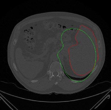
www.nature.com/scientificreports/

                                            Figure 1.  Illustration of the general MDP pipeline using segmentation as the application of interest. The red
                                            arrow is for the training phase only and the blue arrows are shared between the training and testing phase.
                                            In this example, we segment and register a liver 3D surface mesh to the CT image. The scalar N denotes the
                                            number of vertices, the point feature comprises the normalized point coordinates, and the image feature shows
                                            the gray values sampled along the normal directions at each point. The actor network estimates the affine and
                                            non-rigid action given the observation, and the value network calculates the associated Q-values in each case. In
                                            this case, the Q-value for non-rigid action is bigger. Therefore, the non-rigid action will be performed.

                                            Using both the observation ot and action set at ∈ At , the value networks predict the associated Q value and
                                            determine the policy. Each step is explained in detail in the subsequent sections.
                                                                                                        ∞

                                                           ∗                                                  τ −t
                                                         Q (o, a) = µv (ot , µa (ot ; θa ); θv ) = max E
                                                                                                    π
                                                                                                            γ      rt |o = ot , at = µa (ot ; θa ), π   (5)
                                                                                                               τ =t

                                            Observation encoding. The observation encoding ot is generated by sampling the underlying environ-
                                            ment based on current estimates V t . Depending on the target application, an optional pre-processing step (apart
                                            from data normalization) may be applied to the underlying volume. This encoding also depends on whether
                                            we are working with a surface mesh or a point cloud. In the case of 3D surface meshes, we calculate the normal
                                            vector ni,t for each vertex v i,t ∈ V t . We use an equidistant sampling pattern along the normal vector, and extract
                                            pixel values from the environment. When working with unstructured 3D point clouds, we sample a sub-volume
                                            centered on each point v i,t ∈ V t , and extract the associated voxel values from the environment. In both cases, the
                                            sampled values are vectorized and normalized to zero mean, unit standard deviation, to generate the final image
                                            feature. To deal with various voxel spacings in different data, the sampling is done using mm as unit. We also
                                            include the spatial positions of the vertices of the estimate V t (and the corresponding normal vector ni,t if avail-
                                            able) to describe the distribution of the mesh vertices. They are also normalized into unit sphere, and describe
                                            the point feature. The observation encoding ot is a concatenation of these image features and point features,
                                            respectively. An example of observation encoding is shown in Fig. 1.

                                            Actor networks.              The actor network maps the observation to a possible action set At . We define the action
                                            set At as the union of a rigid translation action t t = [tx , ty , tz ]T , scaling action st = [sx , sy , sz ]T , and rotation
                                            action Rt (rx , ry , rz ), and a non-rigid deformation Dt = [d 1 , d 2 , · · · d N ]T ∈ RN×3. Using imitation learning, an
                                            associated actor network µa is trained to predict an action at given a current observation ot . In other words, the
                                            actor network is trained to imitate the behavior of a demonstrator for a given observation. In this context, the
                                            demonstrator provides the optimal rigid or non-rigid action a∗t ∈ A∗t = {R∗t , t ∗t , s∗t , D∗t }. In the training phase,
                                            the ground truth G , describing the correct vertex positions, is given. Therefore, we can calculate the optimal
                                            action a∗t by minimizing Eqs. (6)–(9). The operation ◦ denotes element-wise multiplication, and N (v i,t ) is the
                                            neighbourhood of the vertex v i,t . In case v i,t belongs to a mesh, the N is defined by the adjacent faces of the
                                            mesh. When dealing with point clouds, the k-nearest neighbour algorithm is used to determine the neighbour-
                                            hood N . The regularization term in Eq. (6) makes sure that the deformation vector d i,t for vertex v i,t is similar
                                            to the neighboring deformation vector d j,t for vertex v j,t ∈ N (v i,t ). This ensures the smoothness of the overall
                                            deformation.
                                                                                                              N
                                                                          D∗ = arg min dist(D + V t , G) +                      �d j,t − d i,t �22                     (6)
                                                                                    D
                                                                                                                      i   j∈N (v i,t )

          Scientific Reports |   (2021) 11:3311 |                  https://doi.org/10.1038/s41598-021-82370-6                                                            4

Vol:.(1234567890)
www.nature.com/scientificreports/
N
1
R∗ = arg min (7)
dist Rv i,t , G
R N i
N
1
s∗ = arg min (8)
dist v i,t ◦ s, G
s N i
N
1
t ∗ = arg min (9)
dist t + v i,t , G
t N i
Due to the fact that the observation ot encodes only the neighbourhood, we suffer from a partial obser-
vation effect. To facilitate training of the actor, we normalize the output of the demonstrator. The action
a∗t ∈ A∗t is either normalized to a unit sphere ( D∗ and t ∗), or to a specific range ( s∗ and R∗), and denoted as
A′t = {D′t , t ′t , s′t , R′t (rx , ry , rz )}. In this way, the actor network predicts reasonable actions moving along the same
direction as those of the demonstrator. At the same time, the predicted actions do not overstep the range of the
observation encodings. Subsequently, we introduced an acceleration term β ∈ R+ during training, and define
the target actions a′t,β ∈ A′t,β = {β ◦ D′t , β ◦ t ′t , β ◦ s′t , R′ t (βrx , βry , βrz )}. The action loss function La can thus
be defined as
La = �a′t,β − µa (ot ; θa )�22 + 1 �µa (ot ; θa ) − β�22
′ ′
(10)
at,β ∈At,β
In this equation, the first term denotes the L2 loss computed using the predicted action, and the second term
regularizes the norm of the action to β . We also introduce an auxiliary loss that computes the distance between
the predicted (V t ) and ground truth (G) vertices as,
2
Ld = dist(v i,t , G) (11)
N v ∈V
i,t t
g
The scalar 1 and 2 are the Lagrangian multiplier. The combined loss evaluated as La = La + Ld , was used
for training. Furthermore, we adopted a multi-task training strategy for the actor network µa, based on the rigid
and non-rigid actions to be estimated. This improved network stability during training and reduced the overall
computational complexity. The network architecture is depicted in Fig. 2.
Value network. In order to determine the best action a∗t in the predicted action set At using the actor net-
work µa, such that the sum of current and expected cumulative future reward is maximized, a value network is
trained to estimate the Q-value for each action at . To this end, we use the Q-learning framework and define the
value network as µv (ot , at ; θv ), where θv represents the associated hyperparameters. The instant reward at step
t is expressed as
N N
1 1
rt = dist(v̂ i,t , G) − dist(v i,t , G) (12)
N i N i
where v̂ i,t denotes the current estimate of v i,t applying predicted action at . This indicates, the relative reduction
of the distance between estimates and the ground truth. The optimal action-value function Q∗ is defined using
Eq. (1), and the loss function can be found in Eq. (2). To facilitate training of the value network, we used a double
deep Q-network (DDQN)34, where a separate target network µ− v (ot , at ; θ ) is introduced to approximate Q as,
− ∗
Q∗ ≈ rt + γ max µ− −
v (ot+1 , at+1 ; θ ) (13)
at+1
In Eq. (13), θ − represents the hyperparameters of the target network. Both networks share the same architecture,
but θ − is updated slowly i.e. once every few iterations, while θv is updated every iteration. This strategy contributes
to the overall convergence of the network(s), during training.
We determine the boundary condition of the Q-value to facilitate training of the value and target network.
The action at is estimated using the actor, and the magnitude of the action is constrained by the normalization
and the acceleration factor β . Accordingly, we approximate the upper bound of the reward function as, rt+ ≈ β .
1 g
Furthermore, we approximate the average action √ loss as L̄ = 2 La . This in turn enables us to approximate the
−
lower bound of the reward function, rt ≈ − L̄ > −β . As the reward function is bounded, we determine the
boundary condition of the Q-value using sequence limit, as expressed in,
rt− rt+
< Q∗ < min , dmax (14)
(1 − γ ) (1 − γ )
Here, dmax , denotes the maximal distance between the estimates and the ground truth. The value of dmax can be
calculated according to the data augmentation strategy employed.
Although we have shown in Eq. (14) that the Q-value is bounded, it is not practical to set the number of steps
t → ∞, during inference. This is why we employ two termination criteria for the action sequence chosen by the
Scientific Reports | (2021) 11:3311 | https://doi.org/10.1038/s41598-021-82370-6 5
Vol.:(0123456789)www.nature.com/scientificreports/
Figure 2. Illustration of the network architecture for the actor network (top) and value network (bottom),
respectively. Feature maps are represented as boxes. The scalar N denotes the number of vertices. The dimension
of the observation encoding block depends on the number of sampling points and on the presence of the
normal vector.
value network. First, we introduce tmax as the maximal number of steps in a sequence. This defines the maximum
run-time of the algorithm. The second criterion is that the Q value predicted by the value network should be
greater than Qmin. If the predicted value is less than Qmin, we consider the deformation to be insignificant, and
terminate the sequence.
Data augmentation. We use data augmentation to generate sufficiently rich data for training the actor and
value networks. Data augmentation is applied to both the observation encoding ot and the estimates V t . For the
observation encoding, Gaussian noise was applied to the image features. Data augmentation on the estimates V t
was performed by deforming the ground truth surface meshes G used for training. In order to ensure that the
deformations of the ground truth meshes were realistic, we trained a statistical shape model (SSM) of the target
structure, by template-to-sample registration using the coherent point drift (CPD) algorithm. This registration is
done iteratively, where in the first iteration, a random sample is chosen to be the template. In each iteration, the
template-to-sample registration is performed, and the template is updated by calculating the average model at
the end of each iteration. We then deformed the ground truth G using the modes of variation of the trained SSM,
followed by the application of random affine transformations. Finally, each vertex was randomly jittered using
small displacements, and subsequently, the mesh was smoothed. Note that the point correspondence imposed by
the SSM is applied only to the generated training data. The calculation of the optimal action a∗t of the demonstra-
tor requires no correspondence between the vertices. Therefore, the deformation estimated by the actor remains
independent of point correspondences.
Training. The first step towards training the proposed framework is to train the actor network. To this end,
the Dataset Aggregation (DAGGER) a lgorithm35 was employed to efficiently sample the high dimensional train-
ing data space for a sequential process. The pseudo code for the DAGGER algorithm is presented in Alg 1. In
the first iteration of the DAGGER algorithm, the actor is trained using the training data D generated by the
demonstrator. Subsequently, new data Dπ was gathered by applying the actor, and extracting the observation
and optimal action set generated using the demonstrator. These data Dπ are aggregated with the training dataset
D , for the next iteration of training.
Scientific Reports | (2021) 11:3311 | https://doi.org/10.1038/s41598-021-82370-6 6
Vol:.(1234567890)www.nature.com/scientificreports/
This training scheme is directly applicable to the non-rigid action. When training the network in a multi-
tasking fashion for the rigid actions, we need a criterion to select the action at to further gather training data
Dπ . Here, we select randomly one of the predicted translation, rotation and scale as at.
Following this initial training step, the actor and value networks are jointly trained using the Deep Deter-
ministic Policy Gradients (DDPG) a pproach28. The pesudo code of the DDPG algorithm is presented in Alg. 2.
Here, the value network (referred to as the critic-network i n28) is trained using the DDQN algorithm with an ǫ
-greedy action selection scheme. The gradient of the actor can be calculated using the chain rule to compute the
derivatives of the associated hyperparameters, and update them accordingly. As our actor network is pre-trained
using imitation learning, we update our actor at a much slower rate than the value network.
Network architecture. The proposed architecture for the actor and value network is shown in Fig. 2. Both
networks have shared layers designed to extract high-level features from the encoded observations. This shared-
layer architecture was inspired by the P ointNet36, where a dense layer was used to extract vertex-wise local
features. These features are merged using a pooling layer, enabling inter-vertex global features to be learned. The
extracted global features are permutation invariant, and therefore do not pose any restrictions on the structure
of the neighbourhood. The global feature is repeated and aggregated with the local vertex-wise features using
skip connections, as done in the U-Net. The output layer for the actor network, predicts the non-rigid action
as a deformation vector for each vertex, and the affine action in the form of an affine transformation with nine
degrees of freedom. Consequently, the output layer is constructed to fit the outputs of the actor, where, for the
rigid action, an additional pooling layer is used to encode each action (i.e. rotation, translation and scaling) as a
vector. For the value network, the predicted actions are considered as additional input and concatenated with the
global inter-vertex features extracted using the shared network architecture. The outputs of the value network are
the Q-values estimated for the associated actions.
Results
We evaluated our method for two different tasks, namely, segmentation and registration. For the former, the
performance of our approach was evaluated for mono- and multi-modal liver segmentation and compared to a
state-of-the art approach, namely the 3D U-Net. In addition, the registration performance of our approach was
evaluated for the challenging task of intra-operative brain shift compensation based on multi-modal images.
Furthermore, we investigated the effect of the acceleration factor β used when training the value network, assessed
Scientific Reports | (2021) 11:3311 | https://doi.org/10.1038/s41598-021-82370-6 7
Vol.:(0123456789)www.nature.com/scientificreports/
Dice Parameters Runtime
[%]
Dataset No. Algorithm AVG ± STD [M] [s]
Anatomy3 20 Our method 90.8 ± 0.7 2.7 1
CT 3D U-Net 90.5 ± 3.6 16.1 60
SilverCopus 51 Our method 89.9 ± 0.6 2.7 1
CT 3D U-Net 89.1 ± 3.9 16.1 60
Table 1. Mono-modal liver segmentation accuracy, trainable parameters (in millions), and run-time
comparison for the Anatomy3 and SilverCopus datasets. The number of parameters for the proposed methods
is the sum of actor and value networks.
the convergence of the algorithm, and analyzed its computational complexity. All computations during both
training and evaluation were performed on the same machine using an NVIDIA GTX 1070 GPU.
Mono‑modality image segmentation. In the first set of experiments, evaluating mono-modal segmen-
tation performance, we trained our framework using the Visceral Anatomy337 CT datasets, comprising 20 CT
volumes with ground truth segmentations for the liver. The dataset was partitioned into training, validation,
and test sets, using a split of 16 : 2 : 2. The 3D U-Net was used as a baseline for comparison with our approach.
To this end, it was trained and evaluated using the same samples. All volumes were normalized such that their
intensity values are within the range of [0, 1]. Due to clinical runtime requirements and hardware restrictions
imposed by the target application, the input to the 3D U-Net had to be resampled. To this end, we cropped the
original volumes to ROIs centered around the liver, and resampled the ROIs to a resolution of 128 × 128 × 128.
A DICE loss function, as proposed i n15, was used to train the 3D U-Net. In contrast, for the proposed method
we could use the volumes in their original resolution and no cropping was performed. As described above, we
augmented the data when training the actor and value networks. This was done by first training an SSM of the
liver using each training sample (via template-to-sample registration using CPD). Subsequently, the modes of
the SSM were used to generate realistic deformations of the training samples for augmentation. We sampled
the image feature along the normal vector of each vertex using 1 mm equal distance over 61 points to extract
the gray values. During testing, we placed the template, reshaped using random modes of variation, at different
positions in the volumes. Displacements in the rage of [−40, 40] mm (i.e. approximately half the size of the liver
ROI) in each direction were used. We evaluated both methods by performing a ten-fold cross-validation, using
the Anatomy3 CT dataset. In addition, we tested them on unseen samples from the Visceral Silver-Copus CT
dataset37. The DICE coefficient was used as the metric to evaluate the performance. When comparing results, we
state the average (AVG) ± standard deviation (STD) of this metric. The results for both approaches over test sam-
ples from the cross-validation experiments, and the unseen samples from the Visceral Silver-Copus dataset, are
summarized in Table 1.They show that the proposed method managed to outperform the 3D U-Net despite com-
prising significantly fewer parameters (2.7 million as opposed to 16.1 million for the 3D U-Net). Furthermore,
the training of the 3D U-Net took roughly 72 h while the proposed method was trained approximately for 12 h.
Multi‑modality segmentation. In the multi-modality segmentation task, we evaluated the proposed
method on two clinically relevant scenarios. First, we used the models trained in the previous set of experiments
(refer to “Mono-modality image segmentation” section) for liver segmentation in single-energy CT volumes,
and applied them to volumes acquired at different clinical centers, where different scan protocols were followed
to acquire the CT data. This included contrast enhanced CT (CECT) from Visceral Anatomy3, single energy
CT from 3D-IRCADb-01, and dual energy CT (DECT) data collected by our clinical partner. For all datasets,
we only normalized the intensity as introduced in section 3.1. No further pre-processing was used. To evaluate
the robustness of the algorithm, we did not use transfer-learning (i.e. fine-tune the networks) at this stage. We
evaluated for each CT volume in each dataset all ten trained models from ten-fold cross-validation performed
in “Mono-modality image segmentation” section. This was done for both proposed method as well as for the
3D U-Net. Finally, we documented the AVG ± STD DICE score. The segmentation results achieved by the pro-
posed approach and 3D U-Net, for all three types of CT datasets tested, are summarized in Table 2. The results
show that the DICE score of the proposed method was consistently and significantly higher than what could be
achieved with the 3D U-Net.
Second, we evaluated our model using the multi-modal CHAOS challenge dataset. This dataset comprises
a total of 40 contrast enhanced CT (CECT) volumes, 40 T1 in phase MRI volumes, 40 T1 out phase MRI vol-
umes, and 40 T1 SPectral Attenuated Inversion Recovery (SPAIR) MRI volumes of the abdomen. We trained
our network using all modalities simultaneously, without incorporating modality-specific prior knowledge.
This is a challenging task as the appearance and spatial resolution of the data vary significantly. To deal with
the large differences in appearance between MRI and CT, we pre-processed all volumes using a Laplacian of
Gaussian filter (LoG). As depicted in Fig. 3, the LoG filtered images are relatively similar in appearance, unlike
the original images. Each volume was then normalized to unit variance and zero mean. The rest of the pipeline
of the proposed method remained the same, despite the differences in spatial resolution of the images, as all
steps in the proposed method were in the world coordinate system using mm as unit instead of the number
of voxels. We trained the networks using this dataset, then evaluated the performance by applying a ten-fold
Scientific Reports | (2021) 11:3311 | https://doi.org/10.1038/s41598-021-82370-6 8
Vol:.(1234567890)www.nature.com/scientificreports/
Our Method 3D U-Net
DICE [%] DICE [%]
Dataset No. AVG ± STD AVG ± STD
Anatomy3 CECT 20 82.6 ± 7.6 72.4 ± 9.9
3DIrcad 20 82.3 ± 9.0 59.4 ± 11.1
Dual Energy CT 45 86.5 ± 3.5 60.5 ± 10.5
Table 2. Multi-modal liver segmentation accuracy using pre-trained CT model for Anatomy3 CECT, 3DIrcad
and DECT datasets acquired with different scan protocols, and cross-validation on CHAOS CT-MR dataset.
The accuracy of CHAOS CT-MR dataset is further broken down into individual modalities.
Figure 3. An example of the CHAOS multi-modal segmentation dataset. The top row shows the original
images (CECT, MRI T1 in-phase, MRI T1 out-phase, MRI T2-SPIR). The middle row shows associated
pre-processed images using the LoG filter. The bottom row displays the original images together with the
segmentation estimates (green) and ground truth (red).
cross-validation. In the ten-fold cross-validation, we formed 40 sets, each comprising a volume of each modality.
In other words, each set included one CECT volume, one T1 in phase volume, one T1 out phase volume, and one
T1 SPAIR volume. The ratio between training, validation and testing for these 40 sets was 32:4:4. As shown in
Fig. 3, using the proposed method, a single trained network can segment input volumes of different modalities.
The segmentation performance is comparable for all different modalities despite the difference in appearances
and spatial resolutions.
Registration. For the registration application, we picked brain-shift compensation32. The network was
trained and cross-validated using the Correction of Brainshift with Intra-Operative Ultrasound (CuRIOUS)
MICCAI challenge 2018 training dataset. In total 20 datasets were used. They were partitioned into training,
validation, and testing, using a split of 16:2:2. In this setting, we encoded the observation by sampling a 7 × 7 × 7
sub-volume centered at each landmark without any preprocessing step and relied on the actor to estimate asso-
ciated deformation vectors. Since the volume was registered to the pre-operative data via an optical tracker on
the ultrasound probe during the intervention38, we only used the non-rigid action in this setting. Therefore, we
employed only the DAGGER to train the actor but no value network was involved. The actor network architec-
ture was the same as illustrated in Fig. 2 with small variations in the input layer due to difference in observation
encoding. We further changed the base number of feature kernels from 64 to 32. As the number of landmarks
Scientific Reports | (2021) 11:3311 | https://doi.org/10.1038/s41598-021-82370-6 9
Vol.:(0123456789)www.nature.com/scientificreports/
Landmarks Mean distance (range) Mean distance (range)
ID Number Initial in mm Corrected in mm
1 15 1.82 (0.56–3.84) 0.88 (0.25–1.39)
2 15 5.68 (3.43–8.99) 1.01 (0.42–2.32)
3 15 9.58 (8.57–10.34) 1.10 (0.30–4.57)
4 15 2.99 (1.61–4.55) 0.89 (0.25–1.58)
5 15 12.02 (10.08–14.18) 1.78 (0.66–5.05)
6 15 3.27 (2.27–4.26) 0.72 (0.27–1.26)
7 15 1.82 (0.22–3.63) 0.86 (1.72–0.28)
8 15 2.63 (1.00–4.15) 1.45 (0.73–2.40)
12 16 19.68 (18.53–21.30) 2.27 (1.17–4.31)
13 15 4.57 (2.73–7.52) 0.96 (0.31–1.44)
14 15 3.03 (1.99–4.43) 0.87 (0.31–1.92)
15 15 3.32 (1.15–5.90) 0.69 (0.23–1.17)
16 15 3.39 (1.68–4.47) 0.83 (0.34–1.96)
17 16 6.39 (4.46–7.83) 0.96 (0.31–1.61)
18 16 3.56 (1.44–5.47) 0.89 (0.33–1.33)
19 16 3.28 (1.30–5.42) 1.26 (0.41–1.74)
21 16 4.55 (3.44–6.17) 0.85 (0.26–1.33)
23 15 7.01 (5.26–8.26) 1.08 (0.28–3.40)
24 16 1.10 (0.45–2.04) 1.61 (0.52–2.84)
25 15 10.06 (7.10–15.12) 1.76 (0.62–1.76)
26 16 2.83 (1.60–4.40) 0.93 (0.47–1.44)
27 16 5.76 (4.84–7.14) 2.88 (0.79–5.45)
Proposed 5.37 ± 4.27 1.21 ± 0.55
NiftiyReg39 5.37 ± 4.27 2.90 ± 3.59
Table 3. Evaluation of the mean distance between landmarks in MRI and ultrasound before and after
correction.
varied in the data, we introduced a constant, N, chosen such that the maximum number of landmarks could be
accommodated. In case of data with fewer landmarks, random landmarks were copied in the input. This random
copying had no impact on the network, both, during training and testing phase, as the vertex-wise deformation
predicted by the network and the max pooling value remains the same in case of duplicated values. To evaluate
the performance of the proposed method, we used ten-fold cross-validation and applied the trained networks
to the landmarks in the test set. Then we calculated the mean target registration error in mm between estimated
and ground truth position of the all landmarks. We used the NiftigReg method39 as baseline for the registration.
The registration result is shown in Table 3, and examples of the MRI overlaid with registered iUS frames are
depicted in Fig. 4. As we can see, the proposed method compensated the deformation introduced by brain-shift
well.
Computational complexity. To analyze the computational complexity, we consider the trained networks
as O(1) as its parameters are fixed. Our method has a complexity of O(n · m) for both actor and value network,
where n denotes the number of vertices and m denotes the number of features, independent of the 3D vol-
ume resolution. In contrast, 3D U-Net and its variations/extensions have a complexity of O(h · w · d), where h
denotes the height, w denotes the width and d denotes the depth of the volume all in voxels (3D matrix size).
Therefore, for an average case with multiple slices (100–300 slices for an abdomen CT scan and a in-plane matrix
size of 512 × 512), our method is less computational demanding. In terms of time complexity, the processing of
an input mesh with 1K vertices, the actor and value network require approximately 1 GFLOP regardless of the
volume size. At the same time, the base-line 3D U-Net for an input volume size of 128 × 128 × 128 requires 70
GFLOPs.
Speed‑up factor β. We analyzed the actor network w.r.t. the key variable, the speed-up factor β. We chose
the liver segmentation as our target application and investigated the impact of this parameter on the Anatomy3
data. To facilitate the investigation, we chose the actor network for non-rigid registration to evaluate the impact
on performance and general convergence using different β values. We trained the actor network using different
speed-up factors β and evaluated it on one set of test data to investigate its overall impact to the segmentation
performance and general convergence. For a more comprehensive comparison, we also included the one-shot
estimation and one-shot with learning rate. The actor network in one-shot approach learns directly the optimal
action while one-shot with learning rate learns the optimal action multiplied with the learning rate. To study the
effect of different values for β, we evaluated multiple trained actor networks associated with different β values
Scientific Reports | (2021) 11:3311 | https://doi.org/10.1038/s41598-021-82370-6 10
Vol:.(1234567890)www.nature.com/scientificreports/
Figure 4. Two examples of MR Images (grey scale) combined with registered iUS volume overlays (yellow-red
image) using the proposed method. Each row represent a dataset. Left: sagittal view, right: coronal view.
Figure 5. The impact of different acceleration factors β w.r.t to the mean vertex distance of the segmentation.
We also compare results obtained using one-shot prediction (one_shot), vs one-shot with learning rate (one_
shot_lr).
Scientific Reports | (2021) 11:3311 | https://doi.org/10.1038/s41598-021-82370-6 11
Vol.:(0123456789)www.nature.com/scientificreports/
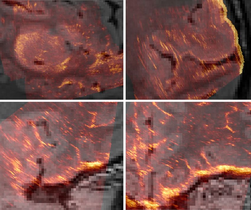
Figure 6. An example of multi-organ segmentation of a CT dataset (left) and warped Visible Human Phantom
segmentation overlay (right).
and ploted the mean vertex distance of the test set over 50 time steps. As shown in Fig. 5, the value of β was
directly correlated to the convergence speed of the algorithm over the time step t.
Discussion and outlook
Our results suggest that the proposed method provides good accuracy and robustness for segmentation and
registration applications in single and multi-modal datasets. While the accuracy for each specific scenario could
be further improved by using specific pre-processing or post-processing methods, we refrained from this, as we
wanted to keep our approach general and flexible. In addition, different data splits and other baseline methods
could be used to find out how the use of other training datasets impacts the proposed method relative to others.
This is, however, part of future work as the number of suitable training datasets currently available to us is limited.
Since the proposed method samples the observation encoding in the volume using absolute dimensions (mm)
instead of voxels as base unit, the algorithm can be readily applied to datasets having different voxel sizes. In
particular, no resampling during both training and application phase is required. This property is especially useful
for multi-modal applications where spatial resolution may vary across different imaging modalities. Also note
that, our method requires a proper computation of an affine transformation matrix between the Right, Anterior,
Superior (RAS+) coordinate system and the voxel coordinate system. In case of clinical datasets, this matrix can
be retrieved or computed using Neuroimaging Informatics Technology Initiative (NII) or DICOM header files.
However, in some segmentation challenge dataset, this relevant information is missing or misleading. In this
case, the proposed method will fail, while methods only relying on voxel data might still work.
In the multi-modal segmentation application we have found that the proposed method still achieves good
performance on CECT and DECT datasets, even when trained on only one type of CT data. On the other
hand, the 3D U-Net struggled with different modalities. One plausible explanation is that the proposed method
does not learn directly from the raw intensity values, whereas the 3D U-Net does. This makes the change of
the intensity values found within the liver, due to contrast agent and different energy levels, detrimental to the
performance of the 3D U-Net. Such changes have less impact on our method, as we learn actions leading to a
correct solution. This robustness was confirmed during the experiments involving the CHAOS dataset, where
LoG pre-processing was used.
We found that large values of β yielded faster convergence but worse accuracy, while small values of β resulted
in slower convergence but higher precision. As expected, the value of β is a trade-off between speed and the
accuracy of the network. Using one-shot, the network diverged after the first iteration. By introducing a learning
rate, we can clearly see that the algorithm stabilized over time.
The introduction of the action normalization and the speedup factor β plays an important role in the training
process. Although it has been shown that the registration can be done using CNN in a one-step a pproach40, this
may not be the optimal approach. If we consider image registration as a sequential energy minimization process,
the one-step approach corresponds to an algorithm finding the solution using a very large learning rate. Such
an algorithm may, however, not converge to a minimum, as shown in Fig. 5. In addition, it may not generalize
well when applied to unseen d atasets41. By normalizing the action, we are effectively setting the step size of the
algorithm to a fixed number. This strategy outperformed a fixed learning rate due to a combination of feature
encoding and the optimization of the loss function. In consecutive steps, the feature encoding remains rather
Scientific Reports | (2021) 11:3311 | https://doi.org/10.1038/s41598-021-82370-6 12
Vol:.(1234567890)www.nature.com/scientificreports/
similar, but the magnitude of the action is constantly changing (due to the learning rate). As a consequence,
the L2 loss function in this ill-posed problem is effectively trying to find an average magnitude of the actions.
As all point correspondences are modeled only implicitly, another potential application of our method is to
register computational phantoms, e.g., the Visible Human (VisHum)42 to CT volumes. This warping propagates
the dense segmentation in the phantom to the CT volume and can facilitate new clinical application, e.g., patient
X-ray dose estimation. In such a case, we train our agent e.g., on lungs, liver, spleen and kidneys. To register the
Visible Human to a CT dataset, we can use the segmentation of the Visible Human as initialization and then
estimate associated deformation vectors of the organs. Afterwards, a dense segmentation field can be interpolated
using these sparse deformation vectors via B-spline interpolation. Using the deformation field, we finally warp the
Visible Human to an arbitrary CT volume. An example of this application is shown in Fig. 6. As we can see, the
visual propagation of the dense segmentation is quite accurate, and our approach can accomplish this in seconds.
In sum, due to its flexibility, robustness, and relatively low computational complexity, the proposed method
provides a promising multi-purpose segmentation and registration framework, particular in the context of
image-guided interventions. In subsequent work, more clinical applications will being investigated
Received: 14 June 2020; Accepted: 14 January 2021
References
1. Gooya, A. et al. Glistr: Glioma image segmentation and registration. IEEE Trans. Med. Imaging 31, 1941–1954 (2012).
2. Wimmer, A., Soza, G. & Hornegger, J. A generic probabilistic active shape model for organ segmentation. Medical Image Computing
and Computer-Assisted Intervention (MICCAI) 26–33 (2009).
3. Mitchell, S. C. et al. 3-d active appearance models: Segmentation of cardiac mr and ultrasound images. IEEE Trans. Med. Imaging
21, 1167–1178 (2002).
4. Zhang, S. et al. Towards robust and effective shape modeling: Sparse shape composition. Medical Image Analysis (MIA) 265–277
(2012).
5. Li, C. et al. A level set method for image segmentation in the presence of intensity inhomogeneities with application to mri. IEEE
Trans. Image Process. 20, 2007–2016 (2011).
6. Lorenzo-Valdés, M., Sanchez-Ortiz, G. I., Elkington, A. G., Mohiaddin, R. H. & Rueckert, D. Segmentation of 4d cardiac MR
images using a probabilistic atlas and the EM algorithm. Med. Image Anal. 8, 255–265 (2004).
7. Fan, J., Yau, D. K., Elmagarmid, A. K. & Aref, W. G. Automatic image segmentation by integrating color-edge extraction and seeded
region growing. IEEE Trans. Image Process. 10, 1454–1466 (2001).
8. Boykov, Y. & Funka-Lea, G. Graph cuts and efficient nd image segmentation. Int. J. Comput. Vis. 70, 109–131 (2006).
9. Adams, R. & Bischof, L. Seeded region growing. IEEE Trans. Pattern Anal. Mach. Intell. 16, 641–647 (1994).
10. Ronneberger, O., Fischer, P. & Brox, T. U-net: Convolutional networks for biomedical image segmentation. Medical Image Comput-
ing and Computer-Assisted Intervention (MICCAI) 234–241 (2015).
11. Goodfellow, I., Bengio, Y. & Courville, A. Deep Learning (MIT Press, 2016). http://www.deeplearningbook.org.
12. Suzuki, K. et al. Computer-aided measurement of liver volumes in CT by means of geodesic active contour segmentation coupled
with level-set algorithms. Med. Phys. 37, 2159–2166 (2010).
13. Çiçek, Ö., Abdulkadir, A., Lienkamp, S. S., Brox, T. & Ronneberger, O. 3d u-net: learning dense volumetric segmentation from
sparse annotation. In International Conference on Medical Image Computing and Computer-Assisted Intervention 424–432 (Springer,
2016).
14. Christ, P. F. et al. Automatic liver and lesion segmentation in CT using cascaded fully convolutional neural networks and 3D
conditional random fields. Medical Image Computing and Computer-Assisted Intervention (MICCAI) 415–423 (2016).
15. Milletari, F., Navab, N. & Ahmadi, S.-A. V-net: Fully convolutional neural networks for volumetric medical image segmentation.
In 2016 Fourth International Conference on 3D Vision (3DV) 565–571 (IEEE, 2016).
16. Chen, H., Dou, Q., Yu, L., Qin, J. & Heng, P.-A. Voxresnet: Deep voxelwise residual networks for brain segmentation from 3d MR
images. NeuroImage (2017).
17. Luc, P., Couprie, C., Chintala, S. & Verbeek, J. Semantic segmentation using adversarial networks. arXiv:1611.08408 (2016).
18. Oktay, O. et al. Attention u-net: Learning where to look for the pancreas. arXiv :1804.03999 (2018).
19. Dalca, A. V., Balakrishnan, G., Guttag, J. & Sabuncu, M. R. Unsupervised learning for fast probabilistic diffeomorphic registration.
arXiv :1805.04605 (2018).
20. Rohé, M.-M., Sermesant, M. & Pennec, X. Automatic multi-atlas segmentation of myocardium with svf-net. In International
Workshop on Statistical Atlases and Computational Models of the Heart 170–177 (Springer, 2017).
21. Juarez, A. G.-U., Selvan, R., Saghir, Z. & de Bruijne, M. A joint 3d unet-graph neural network-based method for airway segmenta-
tion from chest CTS. In International Workshop on Machine Learning in Medical Imaging 583–591 (Springer, 2019).
22. Shah, A., Abramoff, M. D. & Wu, X. Simultaneous multiple surface segmentation using deep learning. In Deep Learning in Medical
Image Analysis and Multimodal Learning for Clinical Decision Support 3–11 (Springer, 2017).
23. Chen, S. et al. Automatic multi-organ segmentation in dual energy CT using 3D fully convolutional network. In (eds. van Gin-
neken, B. & Welling, M.) MIDL (2018).
24. Krebs, J. et al. Robust non-rigid registration through agent-based action learning. In International Conference on Medical Image
Computing and Computer-Assisted Intervention 344–352 (Springer, 2017).
25. Mo, Y. et al. The deep poincaré map: A novel approach for left ventricle segmentation. In International Conference on Medical
Image Computing and Computer-Assisted Intervention 561–568 (Springer, 2018).
26. Mnih, V. et al. Human-level control through deep reinforcement learning. Nature 518, 529 (2015).
27. Silver, D. et al. Mastering the game of go with deep neural networks and tree search. Nature 529, 484 (2016).
28. Lillicrap, T. P. et al. Continuous control with deep reinforcement learning. arXiv:1509.02971 (2015).
29. Ghesu, F. C. et al. Robust multi-scale anatomical landmark detection in incomplete 3D-CT data. Medical Image Computing and
Computer-Assisted Intervention (MICCAI) 194–202 (2017).
30. Ghesu, F.-C. et al. Multi-scale deep reinforcement learning for real-time 3d-landmark detection in CT scans. IEEE Trans. Pattern
Anal. Mach. Intell. 41, 176–189 (2019).
31. Liao, R. et al. An artificial agent for robust image registration. AAAI 4168–4175 (2017).
32. Zhong, X. et al. Resolve intraoperative brain shift as imitation game. In Simulation, Image Processing, and Ultrasound Systems for
Assisted Diagnosis and Navigation 129–137 (Springer, 2018).
33. Toth, D. et al. 3d/2d model-to-image registration by imitation learning for cardiac procedures. Int J Comput Assist Radiol Surg 13,
1141–1149 (2018).
Scientific Reports | (2021) 11:3311 | https://doi.org/10.1038/s41598-021-82370-6 13
Vol.:(0123456789)You can also read