Fast and Compact Image Segmentation using Instance Stixels
←
→
Page content transcription
If your browser does not render page correctly, please read the page content below
Fast and Compact Image Segmentation using Instance Stixels
                                  Thomas M. Hehn, Julian F. P. Kooij and Dariu M. Gavrila1

   Abstract—State-of-the-art stixel methods fuse dense stereo
disparity and semantic class information, e.g. from a Convolu-
tional Neural Network (CNN), into a compact representation of
driveable space, obstacles and background. However, they do not
explicitly differentiate instances within the same semantic class.
We investigate several ways to augment single-frame stixels with
instance information, which can be extracted by a CNN from
the RGB image input. As a result, our novel Instance Stixels
method efficiently computes stixels that account for boundaries
of individual objects, and represents instances as grouped stixels
that express connectivity.
   Experiments on the Cityscapes dataset demonstrate that in-
cluding instance information into the stixel computation itself,
rather than as a post-processing step, increases the segmentation
performance (i.e. Intersection over Union and Average Precision).
This holds especially for overlapping objects of the same class.
Furthermore, we show the superiority of our approach in
terms of segmentation performance and computational efficiency
compared to combining the separate outputs of Semantic Stixels
and a state-of-the-art pixel-level CNN. We achieve processing
throughput of 28 frames per second on average for 8 pixel wide
stixels on images from the Cityscapes dataset at 1792x784 pixels.
Our Instance Stixels software is made freely available for non-
commercial research purposes.

                        I. I NTRODUCTION                                 Fig. 1: Top: Input RGB image (corresponding disparity image
                                                                         not shown). Middle: Semantic Stixels [1] use a semantic
   Self-driving vehicles require a detailed understanding of             segmentation CNN to create a compact stixel representation
their environment in order to react and avoid obstacles as               which accounts for class boundaries (stixel borders: white
well as to find their path towards their final destination. In           lines, arbitrary colors per class). Note that a single stixel
particular, stereo vision sensors obtain pixel-wise 3D location          sometimes covers multiple instances, e.g. multiple cars. Bot-
information about the surrounding, providing valuable spatial            tom: Our Instance Stixels algorithm also accounts for instance
information on nearby free space and obstacles. However,                 boundaries using additional information learned by a CNN
as processing should be as fast as possible, it is essential             and clusters stixels into coherent objects (arbitrary colors per
to find a compact and efficiently computable representation              instance).
of sensor measurements which is still capable to provide
adequate information about the environment [2], [3]. A com-
mon approach is to create a dynamic occupancy grid for
                                                                         Stixels [1]. Yet, obstacles are still just a loose collection of
sensor fusion [4] and tracking [5], which provides a top-
                                                                         upright “sticks” on an estimated ground plane, lacking object
down grid cell representation of occupied space surrounding
                                                                         level information. For example, the car stixels in the middle
the ego-vehicle. Still, directly aggregating depth values into
                                                                         row of figure 1 do not indicate where one car starts and its
an occupancy grid alone would disregard the rich semantic
                                                                         neighboring car ends.
information from the intensity image, and the ability to exploit
                                                                            This paper introduces an object level environment repre-
the local neighborhood to filter noise in the depth image.
                                                                         sentation extracted from stereo vision data based on stixels.
   A popular alternative in the intelligent vehicles domain is
                                                                         Our method improves upon state-of-the-art stixel methods [1],
the “stixel” representation, which exploits the image structure
                                                                         [7] that only consider semantic class information, by adding
to reduce disparity artifacts, and is computed efficiently [6].
                                                                         instance information extracted with a convolutional neural
By grouping pixels into rectangular, column-wise super-pixels
                                                                         networks (CNN) from the input RGB image. This provides
based on the disparity information, stixels reduce the com-
                                                                         several benefits: First, we obtain better stixels boundaries
plexity of the stereo information. Later, class label informa-
                                                                         around objects by fusing disparity, semantic, and instance
tion obtained from deep learning has been incorporated into
                                                                         information in the stixel computation. Second, stixels belong-
the stixel computation and representation, so-called Semantic
                                                                         ing to an object are connected vertically and horizontally
  1 All authors are with the Intelligent Vehicles Group, TU Delft, The   (see bottom image of figure 1) by clustering them based on
Netherlands. Primary contact: d.m.gavrila@tudelft.nl                     semantic and instance information. Third, the processing is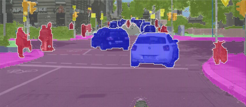
Instances
                                  CNN                                                     Clustering

                                               Instance offsets
        RGB image

                                                                                                                                  Semantics
                                                                            Stixel
                                                                          Computation

        Disparity image
                                               Class probabilities   C

                                                                                                                                  Depth
             2

Fig. 2: Instance stixel pipeline applied to a RGB and disparity input image pair obtained from a stereo camera. The RGB
image is processed by a Convolutional Neural Network (CNN) to predict offsets to the instance centers (HSV color coded) and
per-pixel semantic class probabilities (visualized as color gradient). The class probabilities are fused with the disparity input
image in the Stixel computation to provide a super-pixel representation of the traffic scene, which unifies Semantics, Depth and
additionally Instance output (left images). In the baseline algorithm (Semantic Stixels + Instance, dashed red arrow) the obtained
stixels are clustered based on the instance offsets to assign stixels to instances (not shown). In contrast, our proposed algorithm
(Instance Stixels, blue arrow) fuses the instance offset information with the other two channels in the Stixel Computation.
Subsequently, stixels are also clustered to form instances, but with improved adherence of stixels to instance boundaries (top
right image, arbitrary colors).

more efficient than computing Semantic Stixels [1] and per-          cuts and thus rely on tracking Stixels over time. Stixels are
pixel instance labels separately.                                    also applied in semantic scene segmentation with more general
                                                                     classes than ground, object and sky. For this purpose, semantic
                          II. R ELATED WORK                          information can be obtained by using object detectors for
   The idea of stixels, regarding objects as sticks standing         suitable classes [21] or Random Decision Forest classifiers
perpendicular on a ground plane, was introduced by [6].              [22] and then including that information in the Stixel gen-
The stixel algorithm has found diverse applications in the           eration process. [1] extend this idea by incorporating the
autonomous driving domain. Stixels were used as an integral          output of a Fully Convolutional Neural Network (FCN) in
part of the pipeline for the Berthe Benz drive [8]. [9] develop      the probabilistic stixel framework. They named their approach
a collision warning system using only stereo-based stixels and       Semantic Stixels. Based on Semantic Stixels and focusing on
[10] used stixels to detect small unknown objects, such as           non-flat road scenarios, [7] generalize stixels to also model
lost cargo. The original idea was further extended in [11] to a      slanted surfaces, e.g. not strictly perpendicular to the road
multi-layer representation which used a probabilistic approach,      anymore, including piece-wise linear road surfaces.
i.e. stixels do not need to be connected to the ground plane            Meanwhile, many more deep neural network architectures
anymore. In the multi-layer representation, stixels segment          have been proposed in the computer vision literature to im-
the entire image into rectangular super-pixels, classified as        prove classification and image segmentation tasks on per pixel
ground, object or sky. Additionally, a dynamic programming           basis. For instance, Residual Neural Networks [23] facilitate
scheme was presented for efficient real-time computation of          training of deeper networks by learning residual functions.
stixels. For even faster computation, this dynamic program-          Dilated Residual Networks [24] (DRN) improve on this work
ming scheme was then also implemented for the Graphical              by maintaining a higher resolution throughout the fully con-
Processing Unit (GPU) by [12]. In [13] stixels were compared         nected network, while working with the same receptive field.
with other super-pixel algorithms as basis for multi-cue scene       As a consequence, they are useful for applications that require
labeling.                                                            spatial reasoning such as object detection or, as in our case,
   The general stixel framework offers various possibilities         instance segmentation. In order to enforce consistency between
for extensions and modifications. For instance, [14] compared        semantic and instance segmentation, recently the term panoptic
the effects of different methods for initial ground manifold         segmentation was introduced in [25] and has led to further
modeling. Driven by the requirements of autonomous driving,          improvement in the field [26]. Unfortunately, one cannot treat
[15] applied a Kalman filter to track single stixels. Stixel         instance segmentation as a classification problem, as is done
tracking was then further improved by [16]. Yet, stixels are         for semantic segmentation. A main reason is that the number
generally tracked independently and not as parts of an object.       of instances varies per image, which prohibits a one-to-one
In order to obtain object information [17], [18], [19], [20]         mapping of network output channels to instances. Instead
group the Dynamic Stixels based on shape cues and graph              of predicting instance labels directly, [27] trains a CNN to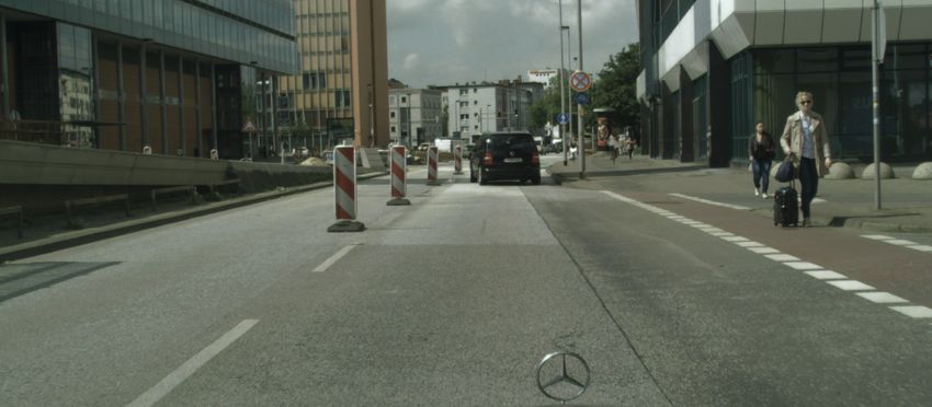
map each pixels in an image onto a learned low-dimensional            •  Clustering stixels from a standard Semantic Stixels
space such that pixels from the same instance map close                  method [1], such that instance offset information is only
together. Object masks are then obtained in post-processing by           considered here at this final clustering step. This baseline
assigning pixels to cluster centers in this space. [28] instead          approach corresponds to the red arrow in Figure 2. In
use supervised learning to map pixels to a specific target               our experiments we shall refer to this combination as the
space, namely the 2D offsets from the given pixel towards                Semantic Stixels + Instance method.
its instance’s center and then rely on clustering all pixels into      • Clustering based on our novel instance-aware stixels
instances. The Box2Pix method [29] uses 2D center offset                 computation from section III-B, see the blue arrow in
predictions for instances, but instead of clustering they are            Figure 2. We name this combination our novel Instance
associated with bounding boxes found through a bounding                  Stixels method.
box detection branch. In order to avoid an additional bounding         Conceptually, Instance Stixels are a natural extension to
box detection branch, [30] learn a clustering bandwidth and         Semantic Stixels as they extend disparity and semantic seg-
confidence per pixel and thereby speed up the grouping of           mentation information with additional instance information to
pixels to instances.                                                compute a compact representation from a stereo image pair.
   Our objective is to create efficient stixel representations      These stixels also receive an object id which groups them into
rather than pixel-accurate instance segmentation in images,         instances.
and to avoid overhead of clustering all pixels into instances
before reducing them to a compact representation. Still, we         A. Stixels
follow insights from the work on per-pixel instance segmen-            In the following, an outline of the derivation of the original
tation to improve stixel computation, deal with the unknown         Stixels and Semantic Stixels framework is presented. For a
number of instances in an image, and enable the clustering          more detailed derivation, see [32] and [1].
of stixels into instances. Building upon our prior conference          1) Disparity Stixels: Following the notation of [32], the full
publication [31], the main contributions are thus summarized        stixel segmentation of an image is denoted as L = {Lu |0 ≤
as:                                                                 u < W } with W being the total number of stixel columns in
   • We present Instance Stixels, a method to include instance      the image. Thus, given a selected stixel width w, it follows
      information into stixels computation, which creates better    that W = imagewwidth . The segmentation of column u contains
      stixels, and allows grouping to instance IDs from a single    Lu = {sn |1 ≤ n ≤ Nu ≤ h} contains at least one but at
      stereo frame.                                                 most height h stixels sn . A stixel sn = (vnb , vnt , cn , fn (v)) is
   • We investigate three different ways to include the instance    described by the bottom and top rows, respectively vnb and vnt ,
      information, and show that adding the information into        that delimit the stixel. Additionally, a stixel is associated with
      the stixel computation itself results in more accurate in-    a class cn ∈ {g, o, s} (i.e. ground, object, sky) and a function
      stance representations than only using it to cluster Seman-   fn which maps each row of the image to an estimated disparity
      tic Stixels or alternatively assigning Semantic Stixels to    value.
      instances using pixel-based methods. Further we compare          The aim is to find the best stixel segmentation L∗ given a
      the trade-off between computation speed and instance          measurement (e.g. a disparity image) D, i.e. it maximizes the
      segmentation performance for these three variations to        posterior probability
      showcase the favorable properties of Instance Stixels.
                                                                                         L∗ = arg max p(L|D).                        (1)
   • We investigate the use of a novel regularizer for Instance                                     L
      Stixels which replaces the former prior term in Stixels.      According to Bayes’ rule, this can be rewritten as
      This simplifies the model and leads to improved instance
      segmentation.                                                                                  p(D|L)p(L)
                                                                                        p(L|D) =                .                    (2)
   • Our entire implementation of the optimized pipeline for                                            p(D)
      Semantic Stixels and Instance Stixels is provided as open-    Here, the normalization factor p(D), constant in L, can be
      source to the scientific community for non-commercial         discarded in the maximization task. Since each column u ∈
      research purposes.                                            {0, ..., W − 1} of the image is treated independently, the MAP
                        III. M ETHODS                               objective can further be simplified:
                                                                                                  W −1
   This section will first briefly summarize the original dispar-                                 Y
ity Stixel and Semantic Stixel formulations in subsection III-A.                 L∗ = arg max            p(Du |Lu )p(Lu ).           (3)
                                                                                            L      u=0
Subsection III-B then explains how to integrate the instance
information from a trained CNN into the stixel computation it-      Here, p(Du |Lu ) denotes the column’s likelihood of the dis-
self for improved stixel segmentation. Finally, subsection III-C    parity data, and p(Lu ) is a prior term modeling the pairwise
will discuss how the instance information can be used to            interaction of vertically adjacent stixels. This is explained in
cluster stixels belonging to the same object.                       more detail in [11].
   The clustering step could be applied to any stixel computa-         Assuming all rows are equally likely to separate two stixels,
tion method. We therefore consider two options:                     the column likelihood term can be written as product of
individual terms for Nu stixels, Lu = {s1 , ..., sNu }. Since              B. Instance Stixels
only disparity values of the rows within each stixel contribute               Instance Stixels expand the idea of Semantic Stixels by
to its likelihood, those terms can in turn be factorized over the          additionally training a CNN to output a 2D estimation of the
rows vnb ≤ v ≤ vnt of each stixel n ∈ {1, ..., Nu }. Hence, the            position of the instance center for each pixel. This estimation
final objective is [32]:                                                   is predicted in image coordinates, as proposed in [29], [28].
                         W −1 Y
                              Nu     vn t                                  More specifically, the CNN predicts 2D offsets Ωp ∈ R2
                                                                           (i.e. x and y direction) per pixel, which are relative to the
                         Y           Y
          ∗
        L = arg max                         p(dv |sn , v)p(Lu ).    (4)
                   L      u=0 n=1 v=vn
                                     b                                     pixel’s location in the image. As a consequence, for all pixels
                                                                           p belonging to the same instance j, adding their ground truth
Here the term p(dv |sn , v) includes different disparity models            offset Ω̂p to the pixel location (xp , yp ) will result in the same
per geometric class. For sky stixels this model is simple:                 instance center location
fsky (v) = 0. The disparity of object stixels is assumed
to be normally distributed around the mean stixel dispar-                                         µ̂j = Ω̂p + (xp , yp ).                    (7)
                         1
                              Pvnt
ity fobject,n (v) = vt +1−v b          b dv . Furthermore, ground
                                 v ′ =vn                                   We refer to such a network as the Offset CNN and an example
                      n     n
stixels rely on a previous estimation of the ground plane                  of its output is visualized in figure 2. The ground truth instance
parameters α (the slope) and vhorizon (horizon estimate in                 centers are defined as the center of mass of the ground
the image), which can be obtained for example from v-                      truth instance masks. Note that instances are commonly only
disparity [33]. The assumed disparity model for ground stixels             considered for certain semantic classes, e.g. cars, pedestrians
fground (v) = α(vhorizon − v) is then linear and the same for              and bicycles. Let I ⊂ N denote said set of instance relevant
all columns. For details, we refer to [12].                                classes. For all other classes, the target offset is (0, 0).
   In practice, the MAP problem (equation 4) is written as an                 Instance Stixels incorporate the Offset CNN prediction into
energy minimization problem by turning the product over prob-              the stixel computation. Let µp denote the instance center
abilities into a sum of negative log probabilities, which is then          estimateP obtained from the CNN for some pixel p, and
solved efficiently through Dynamic Programming (DP) [32],                  µ̄n = p∈Pn µp the mean over all pixels in an instance stixel
[12]. DP will efficiently minimize the energy function                     sn = (vnb , vnt , cn , fn (v), ln , µ̄n ). We model the instance term
                         Nu
                         X                                                 depending on the center estimates of the pixels and the mean
              E(Lu ) =         Ep (sn−1 , sn ) + Ed (sn )           (5)    instance center of the current stixel hypothesis sn :
                         n=1
                                                                                             (P
                                                                                                         ||µp − µ̄n ||22 ,     if ln ∈ I
for many stixel hypotheses Lu = {s1 , ..., sNu }, which                         Ei (sn ) = Pp∈Pn                           2
                                                                                                                                              (8)
                                                                                                   p∈Pn ||µp − (xp , yp )||2 , otherwise.
consists of unary terms Ed (sn ) and pairwise energy terms
Ep (sn−1 , sn ). Intuitively, the unary energy term Ed (sn ) de-           In other words, for instance classes, the instance term favors
scribes the disparity deviation of the disparity models de-                stixels which combine pixels that consistently point to the
scribed above. The pairwise term for n = 1 reads Ep (s0 , s1 )             same instance center. For non-instance classes, i.e. ln ∈ / I,
and is a special case since s0 is not defined. In all other cases,         offsets Ωp = µp − (xp , yp ) deviating from zero contribute to
this pairwise term only evaluates the plausibility of a given              the instance energy term. Without this, classes with instance
stixel segmentation. Note that this in particular means that this          information would generally have higher energy and thus be
pairwise term is independent of the disparity data. We have                less likely than the non-instance classes.
omitted these details here for simplicity [32].                               With the instance energy term, the unary energy becomes
   2) Semantic Stixels: The Semantic Stixels method [1] in-
                                                                                   Eu (sn ) = ωd Ed (sn ) + ωs Es (sn ) + ωi Ei (sn ).       (9)
troduced an additional semantic data term to associate each
stixel with one class label ln ∈ {1, ..., C}. Thus, Semantic               This also introduces weights ωd and ωi for the disparity and
Stixels are characterized by sn = (vnb , vnt , cn , fn (v), ln ). First,   instance terms for more control on the segmentation.
a semantic segmentation CNN is trained on RGB images with                     A useful side effect is that each instance stixel receives a
annotated per-pixel class labels. Then, when testing on a test             mean estimate of its instance center pixel coordinates, which
image, the softmax outputs σ(p, l) for all semantic classes                will be used when clustering stixels into objects, discussed in
l of all pixels p are kept (note that in a standard seman-                 Section III-C.
tic segmentation task, only the class label of the strongest
softmax output would be kept). The unary data term Ed (sn )                C. Clustering stixels with instance information
of the original disparity stixel computation is then replaced                 We now describe how output from an Offset CNN can
by Eu (sn ) = Ed (sn ) + ωl El (sn ), thereby adding semantic              be used in a post-processing step to cluster stixels. Note the
information from the network activations,                                  favorable computational complexity of grouping a low number
                                 X                                         of stixels rather than individual pixels as in conventional
                  El (sn ) = −       log σ(p, ln ).                 (6)    instance segmentation tasks, e.g. 2000 stixels vs. 1.4M pixels.
                                 p∈Pn
                                                                              First, the per-pixel offsets from the Offset CNN are aggre-
Here Pn are all pixels in stixel sn , and ωl a weight factor.              gated into a per-stixel offset estimate by averaging the CNN’s
predictions over the pixels in the stixel (this is already done     and disparity image of a scene and outputs a set of stixels
for Instance Stixels, as noted in Section III-B). Hence, each       comprising information about 3D position, semantic class and
stixel is equipped with an estimate of its instance center in 2D    instance label. Note that in general, Instance Stixels may also
image coordinates, as well as a semantic class label.               operate only on the RGB image without relying on an disparity
   Then, the estimated instance centers and semantic class          image and as a result do not compute the depth of a stixel.
prediction are used to group stixels to form instances. Sep-           The first step in the Instance Stixel pipeline as depicted
arately for each semantic class, we aim to find clusters in         in figure 2 is the CNN which predicts for each pixel the
the estimated instance centers. Note that this condition on         probability of each semantic class and the 2D instance center
the semantic class also qualifies Instance Stixels for panoptic     offset vectors in pixels. On Cityscapes this results in an
segmentation. The final clustering is done using the DBSCAN         output depth of 19 + 2 = 21 channels in total. Any standard
algorithm [34] as it estimates the number of clusters (i.e.         semantic segmentation network architecture could be used as
instances) and performs well when the data has dense clusters.      the basis for the Semantic Segmentation and Offset CNN by
DBSCAN has only two parameters: the maximum distance                increasing the output depth by 2 channels and training those
between neighboring data points ε and the minimum size, as          to predict instance offset vectors. In our implementation, we
in cardinality, γ of the neighborhood of a data point in order      use Dilated Residual Networks [24] (DRN) as our underlying
to consider this point a core point. Additionally, we introduce     architecture due to their favorable properties for these tasks,
a size filter parameter which prevents stixels that are smaller     as discussed in Section II. Furthermore, we exploit the fact
(i.e. cover less rows) than ρ to be considered a core point. This   that, unlike the general method presented in that paper, our
modification prevents small stixels, which lie on the border of     implementation is computes stixels of a fixed width of 8 pixels
two instances, to merge those instances together. Nevertheless,     and remove any upsampling layers in the DRN architecture.
they are assigned to one of those adjacent instances during the     The implementation of the DRN is largely based on the
clustering procedure.                                               PyTorch [36] code provided by the authors of [24]. In order to
                                                                    optimize CNN inference for efficiency, we make use of mixed
D. Unary Regularization
                                                                    precision capabilities of NVIDIA Volta GPUs using the Apex
   The original Stixel MAP formulation considers a prior term       utilities [37] without loss of accuracy.
p(Lu ) (equation 4) which models pairwise interactions of              The second step in the pipeline consists of the actual
vertically adjacent stixels. The prior term contains detailed       stixel computation. For this purpose, we extended the open-
models of the expected segmentation. For example, it models         source disparity Stixel CUDA-implementation introduced in
the probability of a ground stixel to be found below a sky          [12]. Amongst other features, such as the computation of
stixel and vice versa. In the end, the modelled probabilities       Semantic Stixels according to [1] and handling of invalid
are usually estimated heuristically.                                disparity measurements, our extension comprises the Instance
   At the same time, this prior term acts as a regularizer.         Stixels presented here. Techniques to optimize for efficiency,
Without this regularization effect, the resulting stixels tend to   such as the use of prefix sums (aka. cumulative sums), have
be very small simply to fit the data terms as well as possible.     been adapted and reused from the original implementation.
In an extreme case with stixels of a width of 1 pixel, this         [12] provides a detailed explanation of those ideas.
would lead to stixels of also height equal to 1 pixel, which           Lastly, the stixels are clustered based on the mean instance
means in the end that each stixel corresponds to a single pixel.    center estimate. To this end, we utilize the GPU-based DB-
Consequently, the stixel segmentation would not be any more         SCAN implementation of cuML [38] and customize it to
compact than the pixel-wise representation.                         include the size filter ρ described in section III-C.
   We argue that this modeling of pairwise interactions is
                                                                       In summary, all components are implemented on the GPU
especially useful for disparity-based stixels, since there more
                                                                    which reduces the effective number of required host-device
detailed semantic information is missing. Instance Stixels
                                                                    copy operations to two, namely copying the RGB and disparity
however do extract semantic and instance information from
                                                                    images to device memory and retrieving the resulting stixel
the RGB images and thus this modeling may be unnecessary.
                                                                    segmentation from device memory. The source code of our
Therefore, we propose to replace this prior term by a simple
                                                                    implementation is available online1 .
unary regularization term
                                    wR                                                          V. E XPERIMENTS
                    Ep (sn ) = t                             (10)
                               vn + 1 − vnb
                                                                    A. Dataset, metrics and pre-processing
which penalizes small stixels. The regularization constant wR
is the only parameter that needs to be determined and is              The computation of stixels require a RGB camera image
comparable to the different weighting factors of the data terms.    and the corresponding disparity image obtained from a stereo
                                                                    camera setup. We use the Cityscapes dataset [35] for our
                    IV. I MPLEMENTATION                             experiments, as it consists of challenging traffic scenarios.
   We provide an open source Instance Stixels implementation        Further, it provides ground truth annotations for semantic and
which has been optimized for computational performance on
the Cityscapes dataset [35]. As input it requires the RGB            1 Code   available at https://github.com/tudelft-iv/instance-stixels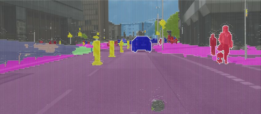
instance segmentation. The performance on these two tasks is all pixel offsets in the image point to the same single point
evaluated using the standard Cityscapes metrics [35]. which would render clustering impossible.
Semantic segmentation performance is measured by the Let j ∈ J denote all ground truth instance masks in an
Intersection-over-Union (IoU) = T P +FT PP +F N , where TP, FP, image, Pj all pixels of that mask and PB all background pixels
and FN denote the number of true positives, false positives which are not part of any instance mask. For all pixels p the
and false negatives over all pixels in the dataset split. An CNN predicts an offset Ωp and using equation 7 thePpredicted
instance mask is considered correct if the overlap with its center µp can be computed. Further, µ̄j = |P1j | p∈Pj µp
ground truth mask surpasses a specific threshold. The Average denotes the corresponding mean of the predicted centers and
Precision (AP) corresponds to an average over the precision for µ̂j the center of mass of the ground truth instance mask. Our
multiple thresholds. Average Precision (AP50% ) only considers offset loss
an overlap of at least 50% as true positive. The metric also
allows to provide confidence score for each instance mask. We
X
a α X α c
X
LO = ||µp − µ̂j ||1 + (µp − µ̄j )2
did not make use of this option and always set the confidence |Pj |1 |Pj |
j∈J p∈Pj p∈Pj
score to 1 for all compared algorithms. αa X
The disparity images provided in the Cityscapes dataset + ||Ωp ||1 (11)
|PB |
exhibit noisy regions introduced due to bad disparity mea- p∈PB
surements at the vertical image edges and the hood of the thus comprises a consistency term based on µ̄j , an accuracy
car. Inaccurate disparity data may harm the performance of term based on µ̂j and a background term. The weights αa and
disparity based Stixels. Although Semantic Stixels are already αc provide the means to find a favorable trade-off between
more robust due to the second modality, we aim to suppress those terms. The full loss L = LO + LS further includes
such effects. Therefore, we crop all images symmetrically (top: a semantic loss LS , namely a 2D cross-entropy semantic
120px, bottom: 120px, left: 128px, right: 128px) to ensure segmentation loss, on the the first 19 semantic output channels.
that our experiments are not influenced by disparity errors. It is important to note that the output (not the input) of
Following [1], we are using the official validation as test set. the CNN is downscaled by a factor 8. We also downscale
Therefore, we split the official training set into a separate the ground truth output by that factor for training. The reason
training subtrain and validation set subtrainval (validation for this is that upscaling, unless nearest neighbor upscaling
cities: Hanover, Krefeld, Stuttgart). is used, introduces interpolation errors that result in a smooth
transition of the offset vectors between two instances. As a
B. Training the CNN
consequence, this would also result in an interpolation of the
The CNN takes an RGB image as input and predicts the predicted means of two neighboring instances at pixels close to
semantic class probabilities and two channels for the offset the borders, which in the end yields worse clustering results.
vectors. Thus, it is a single CNN that provides the output To overcome this issue, we use nearest neighbor upscaling
of the Semantic Segmentation and Offset CNN, which were when passing the predicted images to the Stixel algorithms.
discussed separately in section III. For training, we construct The loss of resolution is compensated by the fact that our
a loss that allows us to steer the focus between consistency Stixels work at a resolution of width 8.
and accuracy of the prediction. Here, we consider a prediction In practice, we found that training the drn d 38 architecture
consistent when all pixels of a ground truth instance mask with αa = αc = 1e − 4 and the drn d 22 architecture with
point towards the same 2D position, i.e. all predictions for αa = 1e − 5 and αc = 1e − 4 worked well. We minimize the
the instance center (equation 7) are the same. Offset accuracy loss function using the Adam optimization [39] (learning rate
is directly measured by the deviation of each single pixel of 0.001, β1 = 0.9 and β2 = 0.999). Further, we apply zero
from the center of mass of the ground truth instance mask. mean, unit variance normalization based on the training data
We argue that, for the predicted offsets, consistency is more to the input data and use horizontal flipping to augment our
important than accuracy. This is best illustrated by an example: training data. The networks were trained for 500 epochs and
consider a single instance in an image and all predicted with a batch size of 20 images. From these 500 epochs, we
offsets of that instance do not point to the center of mass chose the best performing model for each architecture based
of the instance, but instead to a different single point. As on the semantic IoU on the validation set.
a result, this prediction would be consistent, as all offsets
point to the same point, and at the same inaccurate as that C. Hyperparameter optimization
point does not match the ground truth instance mask’s center The stixel algorithms we evaluate offer several hyperparam-
of mass. Despite the fact that this single point is not the eters that require tuning: the weighting of the data terms for
training target, the clustering on this inaccurate, but consistent the Stixel computation ωd , ωs and ωi , as well as the DB-
prediction would work perfectly since all the pixels of the SCAN parameters ǫ, γ and ρ. The stixel framework provides
instance are mapped to a single point and thus form a distinct more parameters from which we set the stixel width to 8
cluster. This observation holds for both the instance-aware pixels throughout our experiments. Remaining parameters are
stixel computation and the clustering. Nevertheless, enforcing set based on recommendations from [32] and [12]. For the
a certain degree of accuracy avoids trivial solutions such as Pixelwise baseline we only need to tune ǫ and γ. Additionally,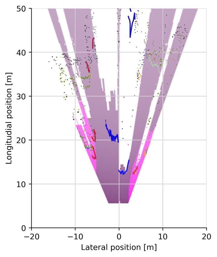
IS 38
            16                                                                                     68       Pixelwise 38
                                                     SS+I 38
            15                                                                                     67                                           IS 38
                                                                                                    SS 38+UPS                                 SS+I 38
             SS 38+UPS
            14

                                                                                         IoU [%]
   AP [%]

                                                                                                   66

            13
             SS 22+UPS                                                IS 22                        65
                                                                                                                                                         SS+I 22
            12       Pixelwise 38                                                                                                                          IS 22
                                                                                                    SS 22+UPS
                                                                    SS+I 22                        64
            11
                 0        5         10          15         20          25       30                      0          5         10          15         20      25     30
                                         Frames per second                                                                        Frames per second
                     (a) Instance performance vs. frames per second.                                        (b) Semantic performance vs. frames per second.

Fig. 3: Trade-off between segmentation performance and processing speed. Each data point represents the average performance
of an algorithm on the Cityscapes validation set (all classes, cropped to 1792x784 pixels). The colors indicate different CNN
architectures (drn d 22 or drn d 38), the symbols differentiate the base algorithm to obtain the instances (triangle: Instance
Stixels, square: Semantic Stixels + Instance, circle: Semantic Stixels + UPSNet, cross: Pixelwise. If the symbol is filled with
color, the unary regularization term was used instead of the pairwise energy term in the stixel computation (section III-D).

                                    CNN            Unary               AP [%]        AP50 [%]               IoU [%]        cat IoU [%]      FPS     Avg. number
                                                   regularization                                                                                   of stixels
                      Pixelwise     drn   d   38   -                   12.5 ± 0.3*   25.3 ± 0.7*            68.2           85.0             0.5     1404928**
                      SS+I          drn   d   22   -                   11.3          25.4                   64.1           80.2             27.5    2095
                      SS+I          drn   d   22   X                   11.3          25.7                   64.6           81.8             28.2    1765
                      SS+I          drn   d   38   -                   14.7          30.3                   66.6           80.8             22.0    1270
                      SS+I          drn   d   38   X                   15.3          31.6                   66.5           81.3             22.1    4795
                      SS+UPS        drn   d   22   -                   12.7          28.5                   64.1           80.2             5.3     2095
                      SS+UPS        drn   d   38   -                   14.1          30.8                   66.6           80.8             5.1     1270
                      IS            drn   d   22   -                   11.8          26.3                   63.8           79.9             27.7    1384
                      IS            drn   d   22   X                   12.6          26.8                   64.3           81.1             28.1    2673
                      IS            drn   d   38   -                   15.8          31.1                   66.4           80.5             22.0    1421
                      IS            drn   d   38   X                   16.3          32.4                   66.9           81.9             22.2    2278

TABLE I: Performance of the Pixelwise baseline and different variations of stixel algorithms that provide instance segmentation
(rows) with respect to various metrics (columns). Results are computed on the Cityscapes validation set (all classes, cropped
to 1792x784 pixels). Best results per metric are highlighted in boldface. * The results of the Pixelwise baseline were averaged
over three runs and are reported with the corresponding standard deviation. All other algorithms are consistent over multiple
runs. ** The resulting segmentation is represented as 1792 · 784 = 1404928 pixels, since no stixels are involved here.

in this baseline the large number of data points requires the                                1) Pixelwise: In this baseline setup, the pipeline as shown
clustering algorithm to process the data in batches which leads                                 in figure 2 is run entirely without stixels, by removing
to non-deterministic results.                                                                   the Stixel Computation. The semantic class is determined
   The parameter tuning is performed using Bayesian opti-                                       according to the largest class probabilities. During the
mization [40] on the subtrainval validation set for 100 iter-                                   clustering step, pixels of the same semantic class are
ations. The score is computed as Semantic IoU+1.5·Instance                                      clustered based on their predicted instance centers.
AP. We weighted Instance AP higher as this is our main focus.                                2) SS+UPS: Represents the combination of state-of-the-art
The optimization is performed separately for each algorithm                                     methods to augment stixels with instance information.
unless noted otherwise.                                                                         Based on a separate instance segmentation method, a
                                                                                                stixel is assigned to an instance by majority vote of the
D. Comparison of algorithmic variations                                                         pixel-level prediction. For this purpose, we utilize the
   To analyze the capabilities of our proposed method, we                                       following state-of-the-art methods: a pretrained instance
vary four different aspects of computing stixels with instance                                  segmentation method called UPSNet [26] and Semantic
information.                                                                                    Stixels [1]. On pixel-level, UPSNet achieves AP perfor-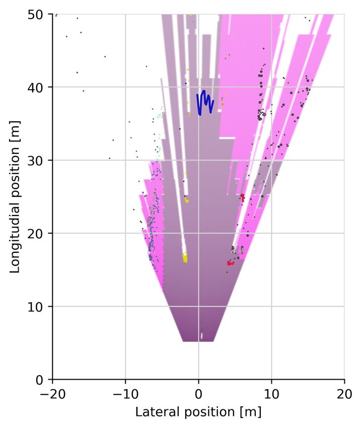
mance of 33.1% on the cropped validation set.               Instance Stixels based on the drn d 38 architecture and using
   3) Semantic Stixels + Instance vs. Instance Stixels (SS+I       the unary regularization outperforms all other stixel-based
       vs. IS): Corresponds to setting ωi = 0, which resembles     algorithms in both segmentation metrics. Only the Pixelwise
       Semantic Stixels [1]), versus ωi > 0 in the stixels         algorithm surpasses this performance in the semantic IoU, but
       computation (see equation 9).                               not the instance AP. The same observations generally also hold
   4) Pairwise vs. unary: Describes whether the stixel com-        for the extended instance and semantic segmentation metrics
       putation takes the pairwise term into account or instead    AP50% and the category IoU [35] as listed in table I.
       regularizes the height of a stixel based on the unary          To a certain degree, segmentation performance comes at
       regularization term as described in section III-D.          a trade-off regarding processing speed. Notably, the speed is
   5) drn d 22 vs. drn d 38: Denotes the different base ar-        mainly determined by the choice of the CNN as well. The
       chitectures of the Dilated Residual Network [24] used       Pixelwise pipeline is by far the slowest algorithm for these
       to predict semantic probabilities and instance offsets.     tasks at only 0.5 frames per second. Stixel methods based
       The architecture drn d 38 is deeper and requires more       on drn d 38 are favorable compared to methods relying on
       memory.                                                     UPSNet, but not as fast as methods based on drn d 22.
Due to the fact that our subtrainval set overlaps with the         Among the same architecture the differences in processing
training set of the UPSNet, we cannot use the subtrainval set      speed are only minor and are listed in table I. Additional
for hyperparameter tuning. Hence, we use the same weights for      analysis showed that the processing speed is steady over all
the Semantic Stixels of SS+UPS as the corresponding SS+I.          frames, regardless of the number of instances or stixels in an
   1) Processing speed vs. Segmentation Performance: In the        image. The complexity of the segmentation, quantified by the
following we compare the different stixel methods for in-          average number of stixels per frame, varies between algorithms
stance segmentation regarding the trade-off of segmentation        exhibiting no obvious correlation. Among the Instance Stixels
performance and processing speed. The main indicators for          the highest average number stixels per frame is at most 2673.
segmentation performance are the instance AP and the se-
mantic IoU as described in section V-A. Processing speed is           2) Qualitative analysis: The consequences of the different
measured as the number of frames the pipeline can process          algorithm variations as described in section V-D are depicted
per second. Here, to compute the frames per second we              in figure 4 when applied on an real traffic scene image from
average the processing time of the frames in the validation        the subtrainval set. Figures 4a and 4b show the input data.
set, which takes into account the processing time of all three     Instance segmentation results in the left column (4 (c),(e),(g)
modules (CNN, Stixel Computation and Clustering, see figure        and (i)) based on the drn d 22 architecture show in general
2), but neglects data loading and visualization. All frames are    more errors than in the right column (4 (d),(f),(h) and (j))
processed sequentially on a NVIDIA Titan V GPU.                    which is based on the drn d 38 architecture. Especially figures
   Figure 3 illustrates the trade-off between processing speed     (g),(i) and (j) show several stixels which overlap two instances.
and instance as well as semantic performance in a com-                Figure 5 visualizes the full results (3D position, semantic
pact manner. Table I extends the figure by providing further       and instance segmentation) of Instance Stixels (drn d 38,
segmentation metrics and also the complexity of the image          unary regularization) on three scenes (columns). Based on the
representation as the average number of stixels per frame on       input RGB images (top row), the CNN predicts the offset
the official Cityscapes validation set.                            vectors (center rows). The offset vectors are visualized in
   In terms of segmentation performance, the illustrations show    HSV color space, where the hue indicates the direction and
that the choice of the network architecture of the CNN,            the saturation the magnitude of the offsets. The fourth row
indicated by the color of the points, has the most prominent       shows the segmentation of the scenes. The overlaid colors
effect (green: drn d 38 and blue: drn d 22). For both seg-         illustrate the semantic class per pixel, whereas the white
mentation metrics, even the best algorithm based on drn d 22       contours around objects mark the borders of instances. The
performing worse than the worst stixel algorithm based on          bottom row shows top down views of the scene based on
drn d 38. Within the same architecture however, Instance           the per stixel disparity information and location within the
Stixels (IS) generally perform better than Semantic Stixels +      input image. In these illustrations the road and the sidewalk
Instance (SS+I) in terms of instance AP, but not always in         are illustrated as polygons. Their boundaries are based on the
terms of semantic IoU. Further, for both algorithms (IS and        ground plane estimation. Sky stixels are discarded and non-
SS+I), using the unary regularization term (filled symbols) sur-   instance stixels are drawn as circles. Their radius indicates the
passes its pairwise counterpart (non-filled symbols) or at least   size of the respective stixel in the image. Stixels of the same
remains on par. Interestingly, the CNN architecture choice         instance are connected by a line. Per column, we only connect
also affects the comparison in instance AP of Instance Stixels     the stixel that are closest to the ego-vehicle. As a result of our
and Semantic Stixels + UPSNet (SS+UPS). For drn d 22, IS           instance segmentation, we can also filter outliers. Specifically,
22 with unary regularization achieves similar instance AP as       we do not include stixels that are further than 3 meters away
SS+UPS 22. For drn d 38, SS+UPS obtains worst instance             from the mean top down position of the instance. Also, we
AP of all stixel methods. The semantic IoU of SS+UPS               removed the stixel artefacts of the Mercedes-Benz Star from
is limited by its SS+I counterpart by construction. Overall,       the top down view based on their position in the image.
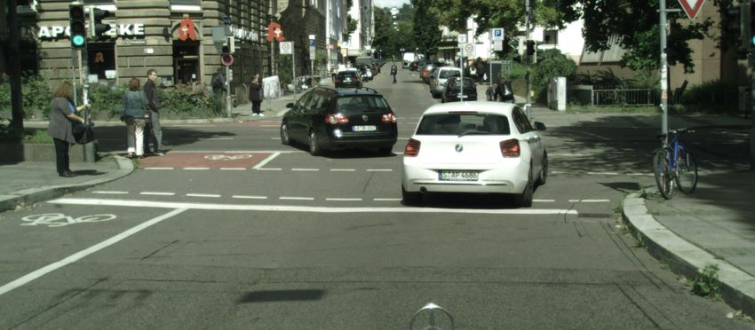
(a) Input: Original image.                                             (b) Input: Disparity image.

               (c) Instance Stixels 22, unary regularization (ours).                  (d) Instance Stixels 38, unary regularization (ours).

                          (e) Instance Stixels 22 (ours).                                        (f) Instance Stixels 38 (ours).

       (g) Semantic Stixels + Instance 22, unary regularization (baseline).   (h) Semantic Stixels + Instance 38, unary regularization (baseline).

                  (i) Semantic Stixels + Instance 22 (baseline).                         (j) Semantic Stixels + Instance 38 (baseline).

Fig. 4: Qualitative analysis of instance segmentation results from Semantic Stixels + Instance (baseline) and Instance Stixels
(proposed algorithm) using different architectures as well as comparing the pairwise energy term and the unary regularization.
Figure (a) and (b): The input RGB and disparity image. Below, the left column shows instance segmentation results obtained
using the drn d 22 architecture as basis for the CNN. Likewise, the right column Instances are indicated by arbitrary colors.
White areas denote stixels that cannot be assigned to specific instances, but their predicted semantic class is an instance class.
Black areas indicate that the predicted semantic class is not an instance class.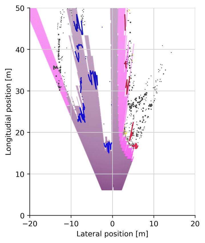
(a) Input RGB image.                             (b) Input RGB image.                             (c) Input RGB image.

         (d) Input disparity image.                       (e) Input disparity image.                       (f) Input disparity image.

     (g) Intermediate offset prediction.              (h) Intermediate offset prediction.              (i) Intermediate offset prediction.

  (j) Instance Stixels, unary regularization.     (k) Instance Stixels, unary regularization.      (l) Instance Stixels, unary regularization.

(m) Instance Stixels 38, unary regularization.   (n) Instance Stixels 38, unary regularization.   (o) Instance Stixels 38, unary regularization.

Fig. 5: Illustration of stixel segmentations including spatial top down view of the scene. Each column is a separate scene,
the top two rows show the corresponding inputs, the center row shows the offsets predicted by the CNN and the bottom two
rows visualize the output of Instance Stixels (drn d 38, unary regularization). In the third row from the top, the overlaid
color indicates the semantic class of a stixel, whereas the white contour around objects indicate the segmented instances. The
last row shows the top view of the scene. Instances are visualized as lines, road and sidewalk stixels are plotted as polygons
based on the obtained ground plane estimation. Stixels of class sky are discarded in this illustration. All remaining stixels (e.g.
buildings and poles) as points and their radius indicates the stixels size.
VI. D ISCUSSION rounding, contained in Instance Stixels can benefit subsequent
utilization in an autonomous driving pipeline. For example,
Results presented in section V-D show that adding the in- Instance Stixels provide a rich and efficient representation for
stance term, that distinguishes IS and SS+I, increases instance path planning, object tracking, and mapping.
AP. Minor drawbacks in terms of semantic IoU may be due to
hyperparameter optimization which values instance AP more VII. C ONCLUSIONS
than semantic IoU. Despite the increased instance AP, the This paper introduced Instance Stixels to improve stixel
segmentation for far away objects (e.g. the truck in the left- segmentation by considering instance information from a
hand part of figure 4a) and tightly overlapping objects (e.g. CNN, and performing a subsequent stixel clustering step. Our
pedestrians in the left-hand part figure 5a) remain challenging. experiments showed multiple benefits of including the instance
Overall, the choice of the CNN appears to be more important information already in the segmentation step, opposed to only
to the segmentation than the effect of the instance term. No- clustering Semantic Stixels. First, quantitative and qualitative
tably, using a state-of-the-art pixelwise instance segmentation analysis show that Instance Stixels adhere better to object
CNN, such as UPSNet [26], and combining it with Semantic boundaries. Second, Instance Stixels provide more accurate
Stixels falls behind significantly in terms of processing speed. instance segmentation than Semantic Stixels augmented with
UPSNet requires on average 0.15 seconds of processing time instance information from a pixel-level instance segmentation
per frame which on its own yields only 6.6 frames per second. network. Third, Instance stixels still preserve the favorable
Compared to the pixelwise UPSNet result, the instance AP of stixel characteristics in terms of compactness of the segmen-
SS + UPSNet has decreased by more than 50%. A drop in tation representation (on average less than 2673 stixels per
overall accuracy is likely, since the stixels group pixels along image) and computational efficiency (up to 28 FPS at a resolu-
predefined coarse column borders and thus inherently decrease tion of 1792x784). In future work, the integration of additional
the granularity of the prediction. Further, SS do not consider sensor modalities as shown in [41] and temporal information
the instance term introduced for IS, thus stixels may overlap to enforce consistency are potential research directions.
two different instances. UPSNet cannot change this afterwards
which leads to worse performance. Lastly, a pixelwise cluster- ACKNOWLEDGMENT
ing approach shows weak instance segmentation performance
This work received support from the Dutch Science Foun-
at a runtime of 0.5 FPS that is dominated by the clustering
dation NWO-TTW within the Sensing, Mapping and Local-
algorithm suffering from the large amount of points.
ization project (nr. 14892). We further thank the authors of
The benefits of a purely stixels-based instance segmentation
[12] and [24] for kindly providing their code and pre-trained
method however is not only observed in processing speed, but
CNN models to the scientific community.
also in term of segmentation complexity. Pixelwise methods
result in more than 1.4 million independent predictions. Our R EFERENCES
Instance Stixels on average require between 1384 and 2673
[1] L. Schneider, M. Cordts, T. Rehfeld, D. Pfeiffer, M. Enzweiler,
stixels per frame to describe the same amount of pixels. U. Franke, M. Pollefeys, and S. Roth, “Semantic Stixels: Depth is not
This means Instance Stixels reduce the complexity of the enough,” in IEEE Intelligent Vehicles Symposium, 2016, pp. 110–117.
representation by factors between 525.6× - 1015.1×. [2] S. Sivaraman and M. M. Trivedi, “Looking at vehicles on the road:
A survey of vision-based vehicle detection, tracking, and behavior
Aside from image segmentation, Instance Stixels provide analysis,” IEEE Trans. on Intelligent Transportation Systems, vol. 14,
position estimates in 3D space. As a result, top down views no. 4, pp. 1773–1795, 2013.
of a scene can be extracted, similar to a grid map. In contrast [3] M. Braun, S. Krebs, F. Flohr, and D. M. Gavrila, “Eurocity persons:
A novel benchmark for person detection in traffic scenes,” IEEE Trans.
to a grid map, our representation is continuous and does not on Pattern Analysis and Machine Intelligence, vol. 41, no. 8, pp. 1844–
discretize 3D space. In this top down representation, imperfect 1861, Aug 2019.
disparity measurements, become apparent, for example in that [4] D. Nuss, T. Yuan, G. Krehl, M. Stübler, S. Reuter, and K. Dietmayer,
“Fusion of laser and radar sensor data with a sequential monte carlo
the back of cars do not appear as straight lines. Further, it bayesian occupancy filter,” in IEEE Intelligent Vehicles Symposium,
also show the inaccuracies of the ground plane and horizon 2015, pp. 1074–1081.
estimation, which is here based on v-disparity [33]. In the [5] R. Danescu, F. Oniga, and S. Nedevschi, “Modeling and tracking the
driving environment with a particle-based occupancy grid,” IEEE Trans.
stixel model, stixels above the horizon cannot be classified on Intelligent Transportation Systems, vol. 12, no. 4, pp. 1331–1342,
as ground. This leads to artefacts as seen on the road behind 2011.
the two cars in figure 5j. As the ground plane estimation is [6] H. Badino, U. Franke, and D. Pfeiffer, “The stixel world - a compact
medium level representation of the 3d-world,” in 31st DAGM Symposium
crude, the polygons of the road stixels overlap sometimes with on Pattern Recognition. Berlin, Heidelberg: Springer-Verlag, 2009, pp.
stixels of obstacles. Combining Instance Stixels with LiDAR 51–60.
measurements as shown in [41] may improve both, the depth [7] D. Hernandez-Juarez, L. Schneider, A. Espinosa, D. Vázquez, A. M.
López, U. Franke, M. Pollefeys, and J. C. Moure, “Slanted stixels:
estimation and the ground plane estimation. As this is an Representing san franciscos steepest streets,” British Machine Vision
orthogonal approach, not related to instance segmentation, we Conference 2011, 2018.
made use of our object based representation to for example [8] J. Ziegler, P. Bender, M. Schreiber, H. Lategahn, T. Strauss, C. Stiller, ...,
and E. Zeeb, “Making bertha drive - an autonomous journey on a historic
filter outliers in the depth measurements of a single object. route,” IEEE Intelligent Transportation Systems Magazine, vol. 6, no. 2,
The rich information about both, the static and dynamic sur- pp. 8–20, Summer 2014.[9] W. Sanberg, G. Dubbelman, and P. de With, “From stixels to asteroids: [33] R. Labayrade, D. Aubert, and J.-P. Tarel, “Real time obstacle detection
Towards a collision warning system using stereo vision,” in IS&T in stereovision on non flat road geometry through v-disparity represen-
International Symposium on Electronic Imaging, 2019. tation,” in IEEE Intelligent Vehicle Symposium, 2002, pp. 646–651.
[10] S. Ramos, S. Gehrig, P. Pinggera, U. Franke, and C. Rother, “Detecting [34] M. Ester, H.-P. Kriegel, J. Sander, X. Xu, et al., “A density-based
unexpected obstacles for self-driving cars: Fusing deep learning and algorithm for discovering clusters in large spatial databases with noise.”
geometric modeling,” IEEE Intelligent Vehicles Symposium, pp. 1025– in Kdd, vol. 96, no. 34, 1996, pp. 226–231.
1032, 2017. [35] M. Cordts, M. Omran, S. Ramos, T. Rehfeld, M. Enzweiler, R. Benen-
[11] D. Pfeiffer and U. Franke, “Towards a Global Optimal Multi-Layer son, ..., and B. Schiele, “The cityscapes dataset for semantic urban scene
Stixel Representation of Dense 3D Data,” British Machine Vision understanding,” in IEEE Conference on Computer Vision and Pattern
Conference, pp. 51.1–51.12, 2011. Recognition, 2016.
[12] D. Hernandez-Juarez, A. Espinosa, J. C. Moure, D. Vázquez, and A. M. [36] A. Paszke, S. Gross, S. Chintala, G. Chanan, E. Yang, Z. DeVito, Z. Lin,
López, “GPU-Accelerated real-Time stixel computation,” IEEE Winter A. Desmaison, L. Antiga, and A. Lerer, “Automatic differentiation in
Conf. on Applications of Computer Vision, pp. 1054–1062, 2017. pytorch,” in NIPS-W, 2017.
[13] M. Cordts, T. Rehfeld, M. Enzweiler, U. Franke, and S. Roth, “Tree- [37] NVIDIA Corporation. (visited on: 2019-11-26) Apex: A pytorch
structured models for efficient multi-cue scene labeling,” IEEE Trans. extension: Tools for easy mixed precision and distributed training in
on Pattern Analysis and Machine Intelligence, vol. 39, no. 7, pp. 1444– pytorch. [Online]. Available: https://github.com/NVIDIA/apex
1454, 2017. [38] R. D. Team, RAPIDS: Collection of Libraries for End to End GPU
[14] N. H. Saleem, H. Chien, M. Rezaei, and R. Klette, “Effects of ground Data Science, 2018. [Online]. Available: https://rapids.ai
manifold modeling on the accuracy of stixel calculations,” IEEE Trans. [39] D. P. Kingma and J. L. Ba, “Adam: A method for stochastic optimiza-
on Intelligent Transportation Systems, vol. 20, no. 10, pp. 3675–3687, tion,” in 3rd Int. Conf. Learn. Representations, 2014.
Oct 2019. [40] J. Snoek, H. Larochelle, and R. P. Adams, “Practical bayesian optimiza-
[15] D. Pfeiffer and U. Franke, “Efficient representation of traffic scenes by tion of machine learning algorithms,” in Advances in neural information
means of dynamic stixels,” in IEEE Intelligent Vehicles Symposium, June processing systems, 2012, pp. 2951–2959.
2010, pp. 217–224. [41] F. Piewak, P. Pinggera, M. Enzweiler, D. Pfeiffer, and M. Zöllner,
[16] B. Günyel, R. Benenson, R. Timofte, and L. Van Gool, “Stixels Motion “Improved semantic stixels via multimodal sensor fusion,” in German
Estimation without Optical Flow Computation,” in European Conference Conference on Pattern Recognition. Springer, 2018, pp. 447–458.
on Computer Vision (ECCV). Berlin, Heidelberg: Springer Berlin
Heidelberg, 2012, pp. 528–539.
[17] F. Erbs, A. Barth, and U. Franke, “Moving vehicle detection by optimal
segmentation of the dynamic stixel world,” in IEEE Intelligent Vehicles
Symposium, 2011, pp. 951–956. Thomas Hehn received his Bachelors degree in
[18] F. Erbs, B. Schwarz, and U. Franke, “Stixmentation-probabilistic stixel 2014 and his Master’s degree in 2017, both in
based traffic scene labeling.” in BMVC, 2012, pp. 1–12. Physics from Heidelberg University, Germany. In
[19] ——, “From stixels to objects - a conditional random field based 2018, he received the best paper award of the
approach,” in IEEE Intelligent Vehicles Symposium, 2013, pp. 586–591. German Conference on Pattern Recognition for his
[20] F. Erbs, A. Witte, T. Scharwächter, R. Mester, and U. Franke, “Spider- research on decision tree algorithms done at the
based stixel object segmentation,” in IEEE Intelligent Vehicles Sympo- Heidelberg Collaboratory for Image Processing. He
sium, 2014, pp. 906–911. is currently working toward the Ph.D. degree at Delft
University of Technology. His research focuses on
[21] M. Cordts, L. Schneider, M. Enzweiler, U. Franke, and S. Roth, “Object-
computer vision for autonomous driving.
level priors for stixel generation,” in German Conference on Pattern
Recognition. Springer, 2014, pp. 172–183.
[22] T. Scharwächter and U. Franke, “Low-level fusion of color, texture and
depth for robust road scene understanding,” in IEEE Intelligent Vehicles
Symposium, June 2015, pp. 599–604.
[23] K. He, X. Zhang, S. Ren, and J. Sun, “Deep residual learning for
Julian Kooij obtained the Ph.D. degree in artificial
image recognition,” in IEEE Conference on Computer Vision and Pattern
intelligence at the University of Amsterdam in 2015,
Recognition, June 2016.
where he worked on unsupervised machine learning
[24] F. Yu, V. Koltun, and T. Funkhouser, “Dilated residual networks,” in and predictive models of pedestrian behavior. In
Computer Vision and Pattern Recognition), 2017. 2013 he worked at Daimler AG on path prediction of
[25] A. Kirillov, K. He, R. Girshick, C. Rother, and P. Dollar, “Panoptic vulnerable road users for highly-automated vehicles.
segmentation,” in IEEE Conference on Computer Vision and Pattern In 2014 he joined the computer vision lab of the TU
Recognition, June 2019. Delft, and since 2016 he is an Assistant Professor in
[26] Y. Xiong, R. Liao, H. Zhao, R. Hu, M. Bai, E. Yumer, and R. Urtasun, the Intelligent Vehicles group, part of the Cognitive
“Upsnet: A unified panoptic segmentation network,” in Computer Vision Robotics department at the same university. His
and Pattern Recognition, 2019. research interests include developing novel proba-
[27] B. De Brabandere, D. Neven, and L. Van Gool, “Semantic instance bilistic models and machine learning techniques to infer and anticipate critical
segmentation with a discriminative loss function,” in Deep Learning for traffic situations from multi-modal sensor data.
Robotic Vision, workshop at CVPR 2017. CVPR, 2017, pp. 1–2.
[28] A. Kendall, Y. Gal, and R. Cipolla, “Multi-task learning using uncer-
tainty to weigh losses for scene geometry and semantics,” in IEEE
Conference on Computer Vision and Pattern Recognition, 2018.
[29] J. Uhrig, E. Rehder, B. Fröhlich, U. Franke, and T. Brox, “Box2pix: Dariu M. Gavrila received the Ph.D. degree in
Single-shot instance segmentation by assigning pixels to object boxes,” computer science from Univ. of Maryland at Col-
in IEEE Intelligent Vehicles Symposium, 2018. lege Park, USA, in 1996. From 1997, he was with
[30] D. Neven, B. D. Brabandere, M. Proesmans, and L. V. Gool, “Instance Daimler R&D, Ulm, Germany, where he became a
segmentation by jointly optimizing spatial embeddings and clustering Distinguished Scientist. 2016, he moved to TU Delft,
bandwidth,” in IEEE Conference on Computer Vision and Pattern where he since heads the Intelligent Vehicles group
Recognition, June 2019. as Full Professor. His research deals with sensor-
[31] T. M. Hehn, J. F. P. Kooij, and D. M. Gavrila, “Instance stixels: based detection of humans and analysis of behavior,
Segmenting and grouping stixels into objects,” in IEEE Intelligent recently in the context of the self-driving cars in ur-
Vehicles Symposium, June 2019, pp. 2542–2549. ban traffic. He received the Outstanding Application
[32] D. Pfeiffer, “The stixel world,” Ph.D. dissertation, Humboldt-Universität Award 2014 and the Outstanding Researcher Award
zu Berlin, 2012. 2019, both from the IEEE Intelligent Transportation Systems Society.You can also read