DeepTerramechanics: Terrain Classification and Slip Estimation for Ground Robots via Deep Learning
←
→
Page content transcription
If your browser does not render page correctly, please read the page content below
DeepTerramechanics: Terrain Classification and Slip
                                                Estimation for Ground Robots via Deep Learning

                                                                        Ramon Gonzalez1,2,∗ , Karl Iagnemma1
                                         1 Massachusetts    Institute of Technology, 77 Massachusetts Avenue, Bldg. 35, 02139, Cambridge, MA, USA
                                          2 robonity:   worldwide tech consulting, Calle Extremadura, no. 5, 04740 Roquetas de Mar, Almeria, Spain
arXiv:1806.07379v1 [cs.CV] 12 Jun 2018

                                         Abstract

                                         Terramechanics plays a critical role in the areas of ground vehicles and ground mobile
                                         robots since understanding and estimating the variables influencing the vehicle-terrain
                                         interaction may mean the success or the failure of an entire mission. This research ap-
                                         plies state-of-the-art algorithms in deep learning to two key problems: estimating wheel
                                         slip and classifying the terrain being traversed by a ground robot. Three data sets col-
                                         lected by ground robotic platforms (MIT single-wheel testbed, MSL Curiosity rover,
                                         and tracked robot Fitorobot) are employed in order to compare the performance of
                                         traditional machine learning methods (i.e. Support Vector Machine (SVM) and Multi-
                                         layer Perceptron (MLP)) against Deep Neural Networks (DNNs) and Convolutional
                                         Neural Networks (CNNs). This work also shows the impact that certain tuning param-
                                         eters and the network architecture (MLP, DNN and CNN) play on the performance of
                                         those methods. This paper also contributes a deep discussion with the lessons learned
                                         in the implementation of DNNs and CNNs and how these methods can be extended to
                                         solve other problems.
                                         Keywords: deep convolutional neural network; ground vehicle; machine learning;
                                         MIT single-wheel testbed; MSL Curiosity rover; tracked robot Fitorobot.

                                           ∗ Corresponding author.

                                         Email addresses: ramon@robonity.com, karl.iagnemma@gmail.com

                                         Preprint submitted to arxiv                                                                 June 20, 2018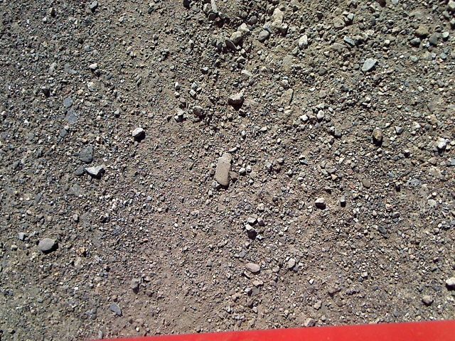
1. Introduction

    Terramechanics was funded in the early 1940s by the necessity to establish a gen-
eral theory studying the overall performance of a machine in relation to its operational
environment: the terrain [57]. Since then, numerous leaps have been accomplished and
terramechanics is broadly used today in many applications: analysis of the performance
of a vehicle over unprepared terrain, ride quality over undulating surfaces, obstacle ne-
gotiation, and study of the performance of terrain-working machinery [33, 50, 58, 59].
Terramechanics is even used for simulating the motion of planetary rovers in Mars
[2, 63].
    Many of the methods found today in the terramechanics literature are inspired by
the pioneering works of Dr. K. Terzaghi, Dr. M.G. Bekker and Dr. J.Y. Wong during
the 1950s and 1960s. The semi-emprical terramechanics model based on their work
has demonstrated a reasonable accuracy for studying vehicle mobility performance
[5, 36, 37, 58]. One of the main aspects of this model is that it requires the knowledge
of certain parameters and variables which are sometimes difficult to measure or esti-
mate online. This aspect is especially important in the context of ground robots where
control and planning methods should consider the physical characteristics of the robot
and its environment to fully utilize the robot’s capabilities [17, 21].
    The limiting factor explained in the previous paragraph partially explains why sev-
eral alternative approaches have been proposed in the field of ground robotics for in-
ferring other variables that also influence the mobility of a robot over a terrain. One
of those broad areas comprises slip estimation. Generally, slip estimation methods
involve either integrating the acceleration measured by an Inertial Measurement Unit
(IMU) [3, 41], or inferring the displacement of the vehicle by using a sequence of im-
ages (i.e. Visual Odometry) [34, 39]. A new area has been recently proposed by the
authors of this paper: it is based on considering slip as a discrete variable and solving
this estimation problem by means of machine learning algorithms [13, 14]. A survey
summarizing the techniques appeared in the literature for slip estimation in the context
of planetary exploration rovers has been already published by the authors in [15].
    Terrain classification represents another wide area within the fields of terramechan-

                                             2
ics and ground robotics. Terrain classification deals with the problem of identifying the
type of the terrain being traversed (or to be traversed) from among a list of candidate
terrains [40]. There are two main bodies of research. The most popular body of re-
search is based on using visual cameras [6, 16, 30, 32]. Terrain classification based
on proprioceptive sensing also comprises numerous references. For example, using
acoustic signals [9, 51], motor current [40] and accelerations [12].
   In parallel to the growing interest in terramechanics and ground robots, another
emerging trend is flooding every area of science and engineering nowadays: deep
learning [18, 24, 26, 25, 27]. Deep learning is becoming popular in countless fields
of the science such as: astronomy where deep learning is applied to locating exo-
planets [46] and finding gravitational lens [43]; satellite image classification [4]; and
medicine where it is used to diagnose certain diseases [49]. In engineering, deep learn-
ing is becoming a must in self-driving cars [8], in face recognition [45], and in speech
recognition [62].
   This paper aims at solving problems found in the areas of terramechanics and
ground robotics by applying the principles of deep learning. As a proof of concept,
deep learning is first applied to two well-known problems: estimating wheel slip and
classifying the terrain being traversed by a robot. In this case, slip estimation is formu-
lated as a classification problem where slip is considered as a discrete variable (i.e. low
slip, moderate slip, and high slip) [13]. Terrain classification is understood as identi-
fying the type of the terrain being traversed, from among a list of candidate terrains
(e.g. gravel, sand, etc.). To date, we are not aware of many publications covering these
specific goals and the two papers found in the literature are only devoted to planetary
exploration rovers (Mars rovers). In [53], the authors employ transfer learning to adapt
a deep neural net (AlexNet) to classify various types of images (Curiosity’s mechani-
cal parts, wheels, etc.). However, this paper neither implement a DNN or a CNN not
compare their performance to other machine learning approaches. In [44], the terrain
classification problem is only solved for Martian terrains. The proposed slip prediction
model neither account for proprioceptive sensor signals nor estimate slip as a discrete
variable.
   This paper is organized as follows. Section 2 reviews the most important concepts

                                            3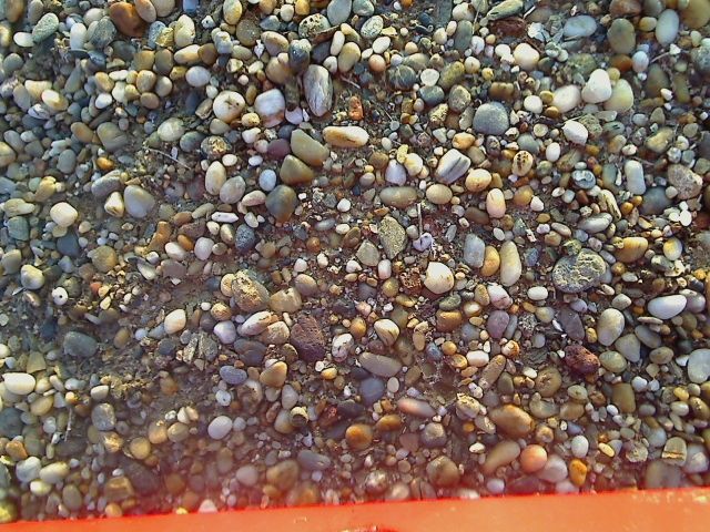
dealing with machine learning and explains the supervised learning methods imple-
mented in this paper. Section 3 overviews the principles of deep learning and intro-
duces the architecture of one of the CNNs implemented in this paper. Section 4 details
the data sets employed in this paper. Section 5 provides experimental results comparing
the performance of traditional machine-learning methods (i.e. SVM and MLP) and the
deep neural networks considered in this work (i.e. DNN and CNN). A deep discussion
of the proposed methodology and the lessons learned while implementing and testing
the deep learning algorithms is addressed in Section 6. Finally, Section 7 concludes the
paper and highlights future efforts.

2. Overview of machine learning

   Machine learning is a branch of computer science based on the study of algorithms
that can learn from and make predictions (generalize) on data [31]. There are two main
types of machine learning algorithms: supervised learning and unsupervised learning.
The supervised learning algorithms aim to minimize some error criterion based on the
difference between the targets (correct responses) and the outputs. On the contrary,
unsupervised learning algorithms exploit similarities between inputs to cluster those
inputs that are similar together. This paper focuses on supervised learning methods.
   One of the most popular supervised learning algorithms is the Support Vector Ma-
chine algorithm (SVM), which was introduced by V. Vapnik in 1992 [52]. It has vastly
demonstrated its suitability in terramechanics mainly dealing with the problem of ter-
rain classification both using proprioceptive signals [22, 56] and exteroceptive signals
[54, 64]. Another popular solution is based on neural networks, which have also proven
to be successful in many areas since McCulloch and Pitts introduced the mathemati-
cal model of a neuron in 1943 [35]. In the context of terramechanics, artificial neural
networks have mostly been applied to terrain classification [40, 55].

2.1. SVM algorithm

   The goal of the SVM algorithm is to find the straight line that leads to the optimal
separation (maximum margin) between the classes or clusters in the input space. The

                                           4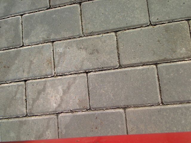
data points that lie closest to the classification line are called support vectors. This
classification line can be written in terms of the input samples as [31]
y = sign(wT x + b), (1)
where y is the output (class label), w is a weight vector, x is an input feature vector,
and b the contribution from the bias weight. Any x value that gives a positive value for
Eq. (1) is above the line and it belongs to the class 0, while any x that gives a negative
value is in the class 1. However, in order to ensure the maximum margin between
both classes, a constrained optimization problem must be formulated to find the w and
b that produce such margin. Thus, this optimization problem must ensure: finding a
decision boundary that classifies well, while also making wT w as small as possible
(widest margin). Mathematically [31]
1
min wT w s.t. ρi (wT xi + b) ≥ 1 ∀i = 1, . . . , l, (2)
2
where ρ is the target or correct response (hand-labeled output), and l is the number of
samples. Notice that both Eqs. (1)-(2) refer to the linear SVM method. Here, a non-
linear SVM formulation has been considered in terms of a radial basis kernel (RBF).
The interested reader can find further details of RBF SVM in [7, 31].
2.2. MLP algorithm
The multi-layer perceptron neural network constitutes one of the most popular feed-
forward artificial neural networks [20, 31, 38]. In this network, the information moves
in only one direction, forward, from the input nodes, through the hidden nodes and to
the output nodes [7]. An MLP usually consists of three layers of nodes (input layer,
hidden layer, and output layer).
The MLP’s algorithm involves a training phase and a recall phase. Initially, the
weights of all neurons in the network are set to a small random number. Next, for each
input vector the activation of each neuron j is computed using an activation function g,
that is [31]
l
wi j xi > 0,
Pl
1 if
X
i=0
= wi j xi ) =
y g( Pl (3)
i=0 0
if i=0 wi j xi ≤ 0.
5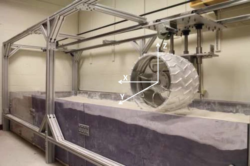
Recall that y is the output (class label), x is the input, w is the neuron weight, and
l is the total number of training samples. After that, each weight in the network is
updated using
wi j = wi j − η(y j − ρ j )wi , (4)
where η is the learning rate and ρ is the target or correct response (hand-labeled
output). Once all outputs of the network are correct (the error with respect to the
targets is zero), the neural network can be used online to predict the class of a new
input. This process is carried out using the activation function previously tuned,
1 i f wi j xi > 0,
Xl
y j = g( wi j xi ) =
(5)
i=0 0 i f w x ≤ 0.
ij i
3. Deep learning framework
Deep learning comprises an extension of the multi-layer perceptron. Recall that
the goal of an MLP is to approximate a function f that maps an input x to a category
y by using a feed-forward neural network [18]. Deep learning extends the traditional
MLP according to the following key principles: (1) the neural network is composed of
many layers and (hidden) neurons (classification layers); and (2) including new layers
in the net such that those layers have the ability to learn and extract features from the
inputs autonomously (feature-extraction layers). This second property means the most
important difference with respect to traditional (shallow) feed-forward neural networks
[31]. In this sense, the term deep of deep learning refers not just to the depth of the
network (many layers of neurons), but to the capability of learning features from the
(raw) data.
One of the most popular and successful architectures in the area of deep learning
is convolutional neural networks (CNNs) [24, 25, 26]. CNNs are characterized by a
grid-like topology composed of a series of layers: convolutional layers, pooling layers,
a dropout layer, a flatten layer, and a set of fully-connected neuron layers. A convolu-
tional layer is a particular type of neural network that manipulates the input image (or
input signal) to highlight certain features, a convolutional layers act as a bank of filters
6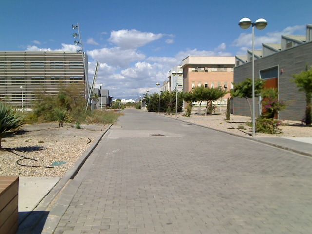
[23, 60]. So, several layers can be stacked in order to highlight different features or
characteristics of the input. After the convolutional layers, a pooling layer is usually
employed. This picks the neurons with the maximum activation value in each grid,
discarding the rest. The convolution layer can be repeated as many times as filters are
desired to apply. Pooling layers are generally placed after every other convolutional
layer or after the whole stack of convolutional layers. The next layer is the dropout
layer which is applied to drop some neurons and their corresponding inputs and out-
puts connections randomly and periodically. This is to ensure that each neuron “learns”
something useful for the network [48]. This dropout layer can be seen as a regulariza-
tion technique for reducing overfitting. Finally, a set of fully-connected (dense) neural
networks are added to the architecture [60, 61].
   Different architectures can be produced by cascading the above-mentioned layers
in various ways. Figure 1 shows one of the deep convolutional neural networks im-
plemented in this work for the terrain classification problem (image classification).
As observed, it is composed of two sets of layers. Feature-extraction layers compris-
ing two 2D convolutional layers with a bank of 32 filters and passing the responses
through a rectified linear function (“ReLu”). A pooling layer creating (2 × 2) grids on
each channel is applied subsequently. After those layers, a new set of two 2D convo-
lutional layers with 64 filters and a polling layer are stacked. The last unit regarding
the feature-extraction part comprises a dropout layer. In order to be able to pass the
output to the dense neural network, the output coming from the dropout layer must be
flatten. The last few layers of the network are conventional fully-connected networks
and the final layer is a “softmax” classifier. This final layer returns the class label for
each input image (e.g. “gravel”, “sand”).

4. Data collection and feature selection

   The generality of the methodology proposed in this work is validated by using
three different data sets. The first dataset represents the lab conditions encountered
in the MIT single-wheel testbed with rippled sandy courses. The second dataset is
composed of images taken by the Mars Science Laboratory rover on Mars (hazcams

                                            7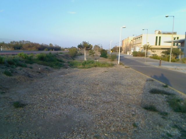
Figure 1: Example of Deep Convolutional Neural Network implemented in this research

and navcams). The third data set comprises images taken by the tracked mobile robot
Fitorobot on Earth (pancam and groundcam).
    At this point, it is interesting to remark that traditional machine learning algorithms
(e.g. SVM and MLP) does not perform well when the input vector(s) used for feeding
the learning model are just raw signals from the sensors. In this sense, a previous
step must be run where the raw data is converted into a different representation (i.e.
filter). This new representation will highlight factors of variation or features in the
observed data [18]. The last part of this section analyzes the features generated for
both the sensor signals used for estimating slip and the images employed for terrain
classification.
    A video showing an experiment with the MIT single-wheel testbed is available at:
https://www.youtube.com/watch?v=kKRSkOrAUdE. Another video with the se-
quence of images used for terrain classification is also available at: http://robonity.
com/video/terrains.mov.

4.1. MIT single-wheel testbed

    Various physical experiments were conducted using a single-wheel testbed devel-
oped by the Robotic Mobility Group (RMG) at MIT, see Figure 2. The system limited
the wheels movement primarily to its longitudinal direction. By driving the wheel and
carriage at different rates, variable slip ratios can be imposed. The bin dimensions are
3.14 [m] length, 1.2 [m] wide, and 0.5 [m] depth.

                                                8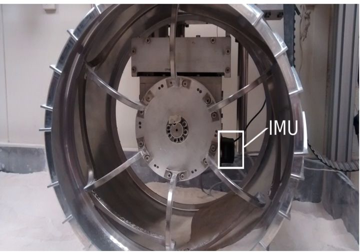
The wheel in use for the experimentation was a Mars Science Laboratory (MSL)
flight spare wheel. The sensing system of the testbed consists of: an IMU (MicroStrain,
3DM-GX2), a torque sensor (Futek, FSH03207), and a displacement sensor (Micro-
epsilon, MK88). Data was recorded at 100 [Hz] in an external computer. A detail of the
placement of the IMU sensor can be seen in Figure 2b. The soil used during testing was
a Mars regolith simulant developed at MIT to replicate conditions being experienced by
the MSL rover on Mars. Numerous experiments were carried out inducing wheel slip
under various operation conditions (i.e., ripple geometries, wheel and pulley velocity
rates) and loading conditions of the carriage pulley. These conditions included small
soil ripples in the path of the wheel to create soil compaction resistance in a manner
similar to what is currently being experienced on Mars by MSL.

    (a) MSL flight spare wheel in MIT’s testbed         (b) Position of the IMU sensor on the MSL wheel

Figure 2: Single-wheel testbed developed by RMG-MIT and used for collecting experimental data. The IMU
constitutes the primary sensor in the proposed methodology.

    For ground-truth purposes, slip was estimated measuring the angular velocity of
the wheel and the angular velocity of the carriage pulley. Outliers were also removed,
for example, when slip had values out of the range [0, 100]. Notice that the dataset
considered in this work comprises a series of ten experiments resulting in a traverse of
approximately 20 [m]. In those experiments the single wheel moved at a fixed velocity
of approximately 0.15 [m/s].
    As explained before, slip has been considered as a discrete variable. In particular,
three discrete classes have been selected regarding the slip estimation problem: low

                                                    9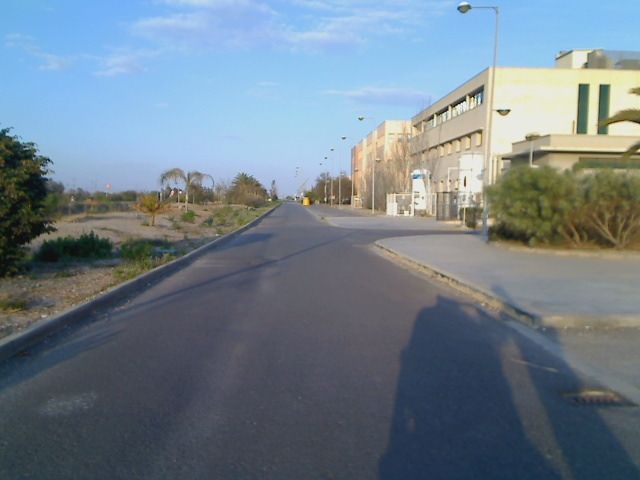
slip (s ≤ 30 [%]), moderate slip (30 < s ≤ 60 [%]), and high slip (s > 60 [%]). The
dataset is composed of 15,000 samples approximately evenly distributed within those
three classes. Further detail can be found in [13].
4.2. MSL Curiosity rover
The second dataset dealing with images in this work has been obtained from the
public NASA’s Planetary Data System (PDS) Imaging Atlas (https://pds-imaging.
jpl.nasa.gov). This dataset contains more than 31 million images, of which 22 mil-
lion are from the planet Mars. The PDS Imaging Atlas allows users to search by mis-
sion, instrument, target, date, and other parameters that filter the set of images. On this
occasion, images have been manually selected and downloaded according to three cat-
egories: “mars clean” (i.e. flat surface with no geometrical hazards), “mars rocks” (i.e.
surface with relatively small rocks and stones) and “mars boulders” (i.e. challenging
surface composed of large rocks). These three categories have been established ac-
cording to the types of terrains and environments that Mars rovers face most frequently
during their operation [1, 2].
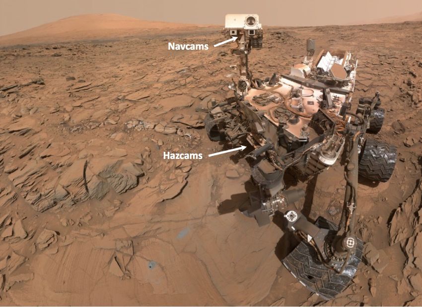
In total, 300 images have been downloaded and distributed evenly in those three
classes. These images were primarily taken by the hazcams and the navcams onboard
Curiosity rover [19, 29]. In the first case, the images represent a close-up look of the
terrain in front of the rover. The images taken by the navcams show the near landscape
surrounding the rover. Figure 3 shows Curiosity’s hazcams and navcams as well as
three representative images of the first data set of images considered in this work.
4.3. Mobile robot Fitorobot
The second data set of images considered in this research was taken by a tracked
mobile robot called Fitorobot that was developed by the University of Almerı́a (Spain)
for experimenting in off-road conditions [17].
As in the previous case, images were taken by two cameras (pancam and ground-
cam). Those images represent five major environments, which are usually found in
the context of ground robotics. More specifically, the categories considered here are:
gravel (ground and panoramic images), sand (ground images), grass (ground images),
10(a) MSL Curiosity rover on Mars
(b) Mars clean (c) Mars rocks (d) Mars boulders
Figure 3: Example images representing three terrain classes used in this research and mobile robot Curiosity
on Mars. Notice that these images have been taken by hazcams and navcams (highlighted in the figure)
pavement (ground and panoramic images), and asphalt (ground and panoramic images)
[16].
A reasonable variety of surface conditions is found for each category. For example,
different grass sizes and differently-sized grains in the gravel terrain. The rectangular
bricks of the pavement surface were not always aligned in exactly the same orientation.
Furthermore, special mention must be made of the fact that the images were taken on
different days and at different hours, so different lighting conditions were ensured. This
second data set of images comprises 800 images evenly distributed within each cate-
gory. Figure 4 shows Fitorobot’s pancam and groundcam as well as six representative
images of this second data set of images.
11(a) Mobile robot Fitorobot
(b) Gravel (pancam) (c) Gravel (groundcam) (d) Asphalt (pancam)
(e) Sand (groundcam) (f) Pavement (pancam) (g) Pavement (groundcam)
Figure 4: Example images representing some terrain classes used in this research and mobile robot Fitorobot
during the experiments
4.4. Feature selection for slip estimation
This section presents the four features that have been chosen to form the feature
input vector to the slip estimation algorithms (i.e. SVM and MLP). The reasoning
behind this choice is based on our experience on this field, see for example [13, 22].
12The first feature is the absolute value of the wheel torque
qi,1 = abs(T i ), (6)
where T i is the i-th instance of motor torque. Notice that during normal outdoor driving,
terrain unevenness leads to variations in wheel torque. This value is increased when
the robot is experiencing moderate or high slip.
The rest of features are collected by an IMU sensor. These features were chosen as
the variance of the Nw element groupings i of the linear acceleration (x-axis), ẋi,Nw , the
degree of pitch (y-axis), φ̇i,Nw , and the vertical acceleration (z-axis), żi,Nw ; see [22] for
further detail of this technique (sliding variance),
qi,2 = var( ẋi,Nw ) = E(( ẋi,Nw − E( ẋi,Nw ))2 ), (7)
qi,3 = var(φ̇i,Nw ) = E((φ̇i,Nw − E(φ̇i,Nw ))2 ), (8)
qi,4 = var(żi,Nw ) = E((żi,Nw − E(żi,Nw ))2 ). (9)
During normal outdoor driving, terrain unevenness leads to variations in those vari-
ables. As in the previous case, this variation is maximized when the robot is experienc-
ing high slip.
4.5. Feature selection for image classification
Traditionally in the field of computer vision, image signatures are employed for
classification purposes. There are several ways to obtain an image signature [11]. One
of the most successful solutions is based on computing a global feature descriptor.
Some of the most well-known global descriptors in the area of computer vision are:
textons [28], GIST [42], and HOG [10]. These descriptors are based on a similar idea,
that is, applying a bank of filters at various locations, scales and orientations to an
image. The average of these filters then gives the image signature [16].
The method employed in this paper is the Histogram of Oriented Gradients (HOG).
As shown in the pioneering paper by [10], the use of HOG descriptor with images
outperforms other image descriptors while considering machine learning algorithms.
This method is based on dividing the image into small spatial regions (cells), for each
cell accumulating a local 1D histogram of gradient directions or edge orientations over
the pixels of the cell. The combined histogram entries form the image signature [10].
135. Experimental results
The main goal of this section is to compare the performance of the two machine
learning algorithms (i.e. SVM and MLP) against the various deep-learning neural nets
considered in this wok (i.e. DNN and CNN).
The results are discussed in terms of two well-known metrics in the field of ma-
chine learning: accuracy and confusion matrix [47]. The hold-out cross-validation
method has been used for selecting the training and testing samples. Additionally, the
performance metrics shown in this section is the average of ten independent runs where
various sizes for the training/testing sets have been considered (e.g. 70/30%, 60/40%,
50/50%). The standard deviation is displayed as well. The experiments have been
run on a standard-performance computer (Intel Core i7, 3 GHz, 16 GB RAM, Ubuntu
16.04). All the software has been implemented in Python using the open source li-
braries: Keras (keras.io), Google’s TensorFlow (tensorflow.org), Scikit-Learn
(scikit-learn.org), and OpenCV (opencv.org).
5.1. Wheel slip estimation based on proprioceptive sensing
This section analyzes the performance of a non-linear SVM algorithm configured
with a kernel based on a radial basis function. The MLP algorithm was tuned with
a hidden layer composed of 30 neurons and a learning rate of 0.01 (as in the previ-
ous case, this configuration has been adopted after running several preliminary experi-
ments).
Regarding the deep learning algorithms (DNN and CNN), the input size has been
established as 4 (four 1D signals coming from the sensors), the batch size was set to
100, the number of epochs was 35. In relation to the DNN algorithm, the network is
composed of one layer of 100 neurons and one final layer of 3 neurons (the three classes
to identify). The activation functions of those layers were “sigmoid” and “softmax”,
respectively. The optimizer used for solving the net was the “adadelta”.
The architecture for the CNN was: three sequential 1D convolutional layers of 128,
64, and 32 filters, respectively. After that, there is 1D pooling layer, a dropout layer
tuned to 0.1, and a flatten layer. The outputs are finally connected to a fully-connected
14neural net composed of two layers, one of 100 neurons and the last layer composed of
3 neurons. In this case, all the intermediate layers have a “relu” activation function, the
activation function for the final layer is “softmax”. This neural net has been solved by
using the optimizer “adadelta” as well.
Figure 5a shows the performance (accuracy) of the learning algorithms. The first
important observation is that the performance of the deep learning algorithms (DNN,
CNN) does not change too much when the signals used for training the algorithms are
filtered or not. On the other hand, the performance of the SVM and MLP algorithms
does depend highly on the way the signals are presented to the algorithm (more than 30
% of difference). This result highlights the key property of deep learning that extract
meaningful information of the input data. Despite the execution of ten independent
experiments with various training and testing set sizes, a small standard deviation is
observed for all the methods. This result reinforces the reliability and generalization of
the learning strategies compared here.
Figures 5b, 5c show the confusion matrices of the SVM (trained with filtered data)
and CNN (trained with raw data) algorithms, respectively. An interesting conclusion
derived from this result is that different algorithms perform differently detecting the
moderate-slip class and the high-slip class. In this case, SVM outperforms CNN while
detecting high-slip samples, but CNN works better than SVM detecting moderate-slip
samples. In any case, the performance of the deep learning approach is certainly re-
markable, specially keeping in mind that SVM is using filtered data and the CNN
algorithm is using raw data coming from the sensors directly (83% vs 88%).
5.2. Terrain classification based on images
This section analyzes the performance of the learning algorithms classifying a set
of grayscale images. All the images have been resized to 128 × 128 pixels. Depending
on the learning algorithm used, the images have been filtered using the HOG algorithm
or have been used directly with no filter (raw pixel values). In particular, raw images
have been used by the two CNN networks implemented here, one DNN algorithm, and
the SVM algorithm. The images filtered with the HOG filter have been used by the
SVM algorithm (same setup than the SVM used with raw images), two different setups
15Performance of the learning algorithms (slip estimation)
100
90
80
70
Accuracy
60
mean
50 std
40
30
20
SVM (raw/filter) MLP (raw/filter) DNN (raw/filter) CNN (raw/filter)
(a) Accuracy (filtered inputs vs raw inputs)
Confusion matrix (SVM) Confusion matrix (CNN)
0.96 0.03 0.01 Low slip 0.90 0.04 0.06 0.8
Low slip 0.8
0.6 0.6
True label
True label
0.22 0.75 0.04 Moderate slip 0.01 0.96 0.04
Moderate slip
0.4 0.4
0.2 0.05 0.31 0.63 0.2
High slip 0.04 0.02 0.94 High slip
p
p
lip
p
p
lip
sli
sli
sli
sli
s
s
w
e
gh
w
e
gh
at
Lo
at
Lo
Hi
Hi
r
r
de
de
Mo
Mo
Predicted label Predicted label
(b) Confusion matrix: SVM (trained with filtered (c) Confusion matrix: CNN (trained with raw
data) data)
Figure 5: Performance of the learning algorithms for estimating wheel slip as a discrete variable (data col-
lected by the MIT single-wheel testbed). Notice that the performance of the algorithms depend on the inputs
(filtered vs raw signals), except for the deep learning algorithms (i.e. DNN, CNN)
16of the MLP algorithm, and the DNN algorithm (same setup than the DNN used with
raw images).
As in the previous section, the non-linear SVM algorithm has been configured with
a radial basis function. Two MLP algorithms have been employed here. One was
tuned with a hidden layer composed of 30 neurons and another one was tuned with two
hidden layers of 15 neurons each. In both cases, the learning rate was set to 0.01.
Regarding the deep learning algorithm (DNN), the input size has been established
as 16384 (128 × 128), the batch size was set to 100, the number of epochs was 35. The
network is composed of one layer of 100 neurons and one final layer of 11 neurons (the
eleven classes to identify). The activation functions of those layers were “sigmoid” and
“softmax”, respectively. The optimizer used for solving the net was the “adadelta”.
With respect to the convolutional neural networks, two different architectures have
been tested. The first architecture (CNN1) was composed of: four sequential 2D con-
volutional layers of 32, 32, 64, and 64 filters, respectively. After that, there is a 2D
pooling layer, a dropout layer tuned to 0.25, and a flatten layer. The outputs are finally
connected to a fully-connected neural net composed of two layers, one of 100 neurons
and the last layer composed of 11 neurons. In this case, all the intermediate layers
have a “relu” activation function, the activation function of the final layer is “softmax”.
This neural net has been solved by using the optimizer “adadelta”. The second con-
volutional neural network (CNN2) was configured as: two 2D convolutional layers,
one pooling layer, two 2D convolutional layers, and another pooling layer. After those
layers, there is a dropout layer tuned to 0.35, and a flatten layer. The outputs are finally
connected to a fully-connected neural net composed of two layers, one of 100 neurons
and the last layer composed of 11 neurons. As in the previous case, all the intermediate
layers have a “relu” activation function, the activation function for the final layer is
“softmax”. This neural net has been solved by using the optimizer “adadelta”.
Figure 6a shows the performance (accuracy) of the learning algorithms. The most
important conclusion is that the performance of the CNN algorithms is quite similar
to the other approaches despite the CNN algorithms are trained with raw images (87%
versus 92% of the best case). Observe the difference in the performance of the SVM
and DNN algorithms when the images are filtered or not (specially dramatic the case
17of the SVM algorithm where performance drops more than 80%). Another interesting
conclusions is related to the behavior of the MLP algorithm. When only one hidden
layer is employed, it leads to the second best accuracy (90%). However, when two
hidden layers are set up, it leads to the second worst accuracy (24%).
Figures 6b, 6c show the confusion matrices of the DNN (trained with filtered data)
and CNN (trained with raw data) algorithms, respectively. As expected after seeing the
plot related to the accuracy, the DNN algorithm classifies almost perfectly every terrain.
An interesting result is obtained by the CNN1 algorithm. It classifies almost perfectly
every terrain, accuracy is higher than 90% in all the cases except for the terrain labeled
as “pavement-ground”. This surprising result is still under research. In any case, this
result does not undermining the satisfactory performance of the CNN algorithm (near
90%).
6. Discussion
The traditional way to operate with machine learning algorithms (i.e. SVM and
MLP) is that the inputs are given as a set of features calculated according to the in-
vestigator’s experience (e.g. filters, global image descriptors). Those derived features
are then fed into the machine learning algorithm. In contrast, deep learning adds gen-
erality to the kind of data that can be processed by a machine learning algorithm as it
does not need any kind of feature extraction step. In this sense, any kind of raw data
coming from the sensors can be directly used for producing a result or making a de-
cision (i.e. signals from IMU sensors or images from stereocameras). This is a major
advantage specially in the area of natural terrain classification where many variables
may affect the image (e.g. lighting conditions, shadows). This advantage can also save
a lot of time while trying to design a pre-processing filter that highlights the main fea-
tures of that signal or image. This property is well observed in this paper by means of
the deep learning algorithms. Figure 7 shows what happens when the best algorithm
used for terrain classification (DNN) is trained with raw images (with no HOG filter).
The performance clearly degrades and many classes are wrongly labeled. On the other
hand, the second deep convolutional neural network implemented for classifying im-
18Performance of the learning algorithms (terrain classification)
100
90
80
70
60
Accuracy
50
mean
40 std
30
20
10
0
SVM+HOG SVM+raw MLP1+HOG MLP2+HOG DNN+HOG DNN+raw CNN1+raw CNN2+raw
Learning algorithms
(a) Accuracy (HOG images vs raw images)
(b) Confusion matrix: DNN (trained with HOG im- (c) Confusion matrix: CNN1 (trained with raw im-
ages) ages)
Figure 6: Performance of the learning algorithms for classifying eleven types of terrains and confusion
matrices of the deep learning algorithms (images captured by MSL Curiosity rover and the tracked robot
Fitorobot). Notice that the performance of the CNN architectures (CNN1, CNN2) perform similarly to the
best algorithms despite they use raw images and the other algorithms use a descriptor for the images (HOG)
ages (CNN2), and trained with raw images, obtains a fairly reasonable result. The
accuracy classifying all the classes is higher than 90% except for the “gravel-pan” and
the “pavement-ground” classes. The accuracy of this CNN algorithm is near 80% and
the accuracy of the DNN trained with raw images is around 65%.
Though the use of deep learning methods result in an attractive solution in the fields
19(a) DNN (trained with raw images) (b) CNN2 (trained with raw images)
Figure 7: Confusion matrices of the DNN algorithm trained with raw images and the second CNN imple-
mented for terrain classification purposes. Compare this result with the one displayed in the previous figure
(specially the DNN case)
of terramechanics and ground robotics, the user must know the following aspects in or-
der to get a proper performance. One of the most important lessons learned during this
research has been related to the number of epochs used for training the deep learning
networks. The point is that that number dramatically impacts on the performance and
the computation time, so a proper balance between the number of epochs and the right
accuracy of the network is needed. In this sense, the network should be trained just the
number of times until the accuracy of the network becomes stable. Figure 8 shows the
evolution of the accuracy of the convolutional neural nets used for estimating slip and
for classifying the terrain. Observe that the accuracy becomes stable when few epochs
are run for the first case (around 10 epochs), but it takes more epochs in the second case
(around 25 epochs). It is important to remark that once the CNN is trained, the testing
time is similar to the other machine learning algorithms (of the order of seconds).
Another critical aspect of convolutional neural nets is related to the training time.
In this sense, the user must be very careful when testing specific aspects of the CNN
as the time to get the result will be very high. In our case, the training time for the
terrain classification problem considering grayscale images is around 3 hours. When
RGB images are used the training time is almost double, around 6 hours. In any case,
20no significant difference has been observed in the performance when RGB images are
used. For that reason, this paper only considers grayscale images.
According to the results obtained when classifying images, there is not a signifi-
cant difference in the two architectures implemented of the convolutional neural nets
(CNN1 and CNN2). This aspect will be further investigated in the future when more
complicated and deeper networks will be analyzed by using Graphical Processing Units
(GPUs).
Other interesting variables that influence the performance of the deep neural net-
works are: (1) the tuning used for the dropout layer; (2) the optimizer used for training
the deep learning network (in this case “adadelta” works better than “sgd” and “mse”);
(3) the activation function at each layer also influences the performance of the whole
neural net (in this case the inner layers used the activation function “relu” and the out-
put layer used the activation function “softmax”).
CNN models accuracy while training
100
90
80
70
60
accuracy
50
CNN images
CNN slip
40
30
20
10
0
0 5 10 15 20 25 30 35
epoch
Figure 8: Evolution of the accuracy of the convolutional neural nets in terms of the number of epochs
(“CNN1” in the previous graphs). In both cases, the net is trained with raw data (sensor signals used for slip
estimation and raw images for terrain classification)
7. Conclusions
This paper aims at applying the trending area of deep learning to the field of ter-
ramechanics and ground robotics. More specifically, state-of-the-art deep convolu-
tional neural networks have been compared to traditional machine learning algorithms
21where a global descriptor of the images and a filter of the signals coming from the
sensors are needed. This comprises a quite different approach to that required by the
deep convolutional neural networks which are fed directly by raw data. The own net-
work extracts the meaningful information from the raw data collected by the sensors.
As explained at the beginning of this paper, the authors are not aware of publications
tackling these same goals in the fields of terramechanics and ground robotics.
Another important aspect derived from this paper is that all the machine learning
algorithms and the deep learning algorithms have been run on a standard-performance
computer with no GPUs. This explains two critical decisions adopted here: (1) the use
of a moderately small image dataset (1100 images), and (2) it has not been possible to
test more complicated architectures for the deep convolutional neural network because
the computation time grows exponentially. For example, in this case, the training time
is around three hours for grayscale images. According to the experience gained during
this research, the performance of the convolutional neural networks will presumably
increase with larger datasets and GPUs. In any case, it is important to remark that this
paper aims at being a proof-of-concept and showing that this trending technology is
ready and can be applied to the particular problems found in terramechanics.
Future efforts will be also devoted to analyzing more challenging phenomena such
as predicting the soil moisture or the thermal inertia of a terrain. For that purpose,
new sensor signals will be considered such as thermal images or signals from ground
penetrating radars.
8. Acknowledgements
The research described in this publication was carried out at robonity’s offices
(Almeria, Spain) and at the Massachusetts Institute of Technology (Cambridge, MA,
USA). This research has been partially funded by NASA under the STTR Contract
NNX15CA25C.
22References
References
[1] Arvidson, R., DeGrosse, P., Grotzinger, J., Heverly, M., Shechet, J., Moreland, S.,
Newby, M., Stein, N., Steffy, A., Zhou, F., Zastrow, A., Vasavada, A., Fraeman,
A., & Stilly, E. (2017). Relating geologic units and mobility system kinematics
contributing to curiosity wheel damage at gale crater, mars. Journal of Terrame-
chanics, 73, 73 – 93.
[2] Arvidson, R., Iagnemma, K., Maimone, M., Fraeman, A., Zhou, F., Heverly, M.,
Bellutta, P., Rubin, D., Stein, N., Grotzinger, J., & Vasavada, A. (2016). Mars
Science Laboratory Curiosity Rover Megaripple Crossings up to Sol 710 in Gale
Crater. Journal of Field Robotics, (pp. 1–24).
[3] Barshan, B., & Durrant-Whyte, H. (1995). Inertial navigation systems for mobile
robots. IEEE Transactions on Robotics and Automation, 11, 328–342.
[4] Basu, S., Ganguly, S., Mukhopadhyay, S., DiBiano, R., Karki, M., & Nemani, R.
(2015). Deepsat – a learning framework for satellite imagery. In Int. Conf. on
Advances in Geographic Information Systems. Seattle, WA, USA.
[5] Bekker, M. (1956). Theory of Land Locomotion. The Mechanics of Vehicle Mo-
bility. (First ed.). Ann Arbor. The Univiersity of Michigan Press, USA.
[6] Bellutta, P., Manduchi, R., Matthies, L., Owens, K., & Rankin, A. (2000). Terrain
Perception for DEMO III. In IEEE Intelligent Vehicles Symposium (pp. 326 –
331).
[7] Bishop, C. (2006). Pattern Recognition and Machine Learning. Information
Science and Statistics. Springer, Berlin, Germany.
[8] Bojarski, M., Testa, D. D., Dworakowski, D., & et al., B. F. (2016). End to end
learning for self-driving cars. ArXiv:1604.07316.
[9] Brooks, C., & Iagnemma, K. (2005). Vibration-based Terrain Classification for
Planetary Exploration Rovers. IEEE Transactions on Robotics, 21, 1185–1191.
23[10] Dalal, N., & Triggs, B. (2005). Histograms of oriented gradients for human de-
tection. In IEEE Computer Society Conference on Computer Vision and Pattern
Recognition. San Diego, CA, USA: IEEE.
[11] Datta, R., Joshi, D., Li, J., & Wang, J. (2008). Image Retrieval: Ideas, Influences,
and Trends of the New Age. ACM Computing Surveys, 40, 1 – 60.
[12] Giguere, P., & Dudek, G. (2009). Clustering Sensor Data for Autonomous Terrain
Identification using Time-Dependency. Autonomous Robots, 26, 171 – 186.
[13] Gonzalez, R., Apostolopoulos, D., & Iagnemma, K. (2018). Slippage and im-
mobilization detection for planetary exploration rovers via machine learning and
proprioceptive sensing. Journal of Field Robotics, 35, 231–247.
[14] Gonzalez, R., Byttner, S., & Iagnemma, K. (2016). Comparison of Machine
Learning Approaches for Soil Embedding Detection of Planetary Exploratory
Rovers. In 8th ISTVS Amercias Conference. Detroit, MI, USA: International
Society for Vehicle-Terrain Systems.
[15] Gonzalez, R., & Iagnemma, K. (2018). Slippage estimation and compensation
for planetary exploration rovers. State of the art and future challenges. Journal of
Field Robotics, 35, 564–577.
[16] Gonzalez, R., Rituerto, A., & Guerrero, J. (2016). Improving Robot Mobility by
Combining Downward-Looking and Frontal Cameras. Robotics, 5, 25 – 44.
[17] Gonzalez, R., Rodriguez, F., & Guzman, J. L. (2014). Autonomous Tracked
Robots in Planar Off-Road Conditions. Modelling, Localization and Motion Con-
trol. Series: Studies in Systems, Decision and Control. Springer, Germany.
[18] Goodfellow, I., Bengio, Y., & Courville, A. (2016). Deep Learning. The MIT
Press, USA.
[19] Grotzinger, J. P., Crisp, J., Vasavada, A., R.C. Anderson, C. B., Barry, R., &
Blake, D. (2012). Mars Science Laboratory Mission and Science Investigation.
Space Science Reviews, 170, 5 – 56.
24[20] Hastie, T., Tibshirani, R., & Friedman, J. (2009). The Elements of Statisti-
cal Learning. Data Mining, Inference, and Prediction. Statistics (Second ed.).
Springer, Germany.
[21] Iagnemma, K., & Dubowsky, S. (2004). Mobile Robots in Rough Terrain. Es-
timation, Motion Planning, and Control with Application to Planetary Rovers.
Springer Tracts in Advanced Robotics. Springer, Germany.
[22] Iagnemma, K., & Ward, C. C. (2009). Classification–based Wheel Slip Detection
and Detector Fusion for Mobile Robots on Outdoor Terrain. Autonomous Robots,
26, 33–46.
[23] Jarrett, K., Kavukcuoglu, K., Ranzato, M., & LeCun, Y. (2009). What is the best
multi-stage architecture for object recognition? In IEEE International Confer-
ence on Computer Vision. Kyoto, Japan: IEEE.
[24] Krizhevsky, A., Sutskever, I., & Hinton, G. (2012). Imagenet classification with
deep convolutional neural networks. In Proc. of the Int. Conf. on Neural Infor-
mation Processing Systems (pp. 1097 – 1105). Lake Tahoe, NV, USA volume 1.
[25] LeCun, Y., Bengio, Y., & Hinton, G. (2015). Deep learning. Nature, 521, 436 –
444.
[26] LeCun, Y., Boser, B., Denker, J., Henderson, D., Howard, R., Hubbard, W., &
Jackel, L. D. (1989). Backpropagation applied to handwritten zip code recogni-
tion. Neural Computation, 1, 541 – 551.
[27] Lee, H., Grosse, R., Ranganath, R., & Ng, A. (2009). Convolutional deep be-
lief networks for scalable unsupervised learning of hierarchical representations.
In International Conference on Machine Learning (pp. 609 – 616). Montreal,
Quebec, Canada.
[28] Leung, T., & Malik, J. (2001). Representing and Recognizing the Visual Appear-
ance of Materials using Three-Dimensional Textons. Int. Journal of Computer
Vision, 43, 29 – 44.
25[29] Maki, J., Thiesses, D., Pourangi, A., Kobzeff, P., Litwin, T., Scherr, L., Elliott, S.,
Dingizian, A., & Maimone, M. (2012). The mars science laboratory engineering
cameras. Space Science Reviews, 170, 77 – 93.
[30] Manduchi, R., Castano, A., Talukder, A., & Matthies, L. (2005). Obstacle De-
tection and Terrain Classification for Autonomous Off-Road Navigation. Au-
tonomous Robots, 18, 81 – 102.
[31] Marsland, S. (2015). Machine Learning. An Algorithmic Perspective. (Second
ed.). CRC Press.
[32] Martinez-Gomez, J., Fernandez-Cabellero, A., Garcia-Varea, I., Rodriguez, L., &
Romero-Gonzalez, C. (2014). A Taxonomy of Vision Systems for Ground Mobile
Robots. Int. J. of Advanced Robotic Systems, 11, 1 – 26.
[33] Mastinu, G., & Ploechl, M. (Eds.) (2017). Road and Off-Road Vehicle System
Dynamics - Handbook. CRC Press, Inc., USA.
[34] Matthies, L., Maimone, M., Johnson, A., Cheng, Y., Willson, R., Villalpando, C.,
Goldberg, S., & Huertas, A. (2007). Computer Vision on Mars. International
Journal of Computer Vision, 75, 67–92.
[35] McCulloch, W., & Pitts, W. (1943). A Logical Calculus of Ideas Imminent in
Nervious Activity. Bulletin of Mathematical Biophysics, 5, 115 – 133.
[36] Meirion-Griffith, G., & Spenko, M. (2011). A modified pressure-sinkage model
for small, rigid wheels on deformable terrains. Journal of Terramechanics, 48,
149 – 155.
[37] Meirion-Griffith, G., & Spenko, M. (2013). A pressure-sinkage model for small-
diameter wheels on compactive, deformable terrain. Journal of Terramechanics,
50, 37 – 44.
[38] Mitchell, T. (1997). Machine Learning. McGraw-Hill.
[39] Nistér, D., Naroditsky, O., & Bergen, J. (2006). Visual Odometry for Ground
Vehicle Applications. Journal of Field Robotics, 23, 3–20.
26[40] Ojeda, L., Borenstein, J., Witus, G., & Karlsen, R. (2006). Terrain Character-
ization and Classification with a Mobile Robot. Journal of Field Robotics, 23,
103–122.
[41] Ojeda, L., Reina, G., & Borenstein, J. (2004). Experimental results from flexnav:
an expert rule-based dead-reckoning system for mars rovers. In IEEE Aerospace
Conference. Big Sky, MT, USA.
[42] Oliva, A., & Torralba, A. (2001). Modeling the shape of the scene: A holistic
representation of the spatial envelope. International Journal of Computer Vision,
42, 145 – 175.
[43] Petrillo, C., Tortora, C., Chatterjee, S., Vernardos, G., & et al., L. K. (2017).
Finding strong gravitational lenses in the kilo degree survey with convolutional
neural networks. Monthly Notices of the Royal Astronomical Society, 472, 1129
– 1150.
[44] Rothrock, B., Kennedy, R., Cunningham, C., Papon, J., Heverly, M., & Ono, M.
(2016). Spoc: Deep learning-based terrain classification for mars rover missions.
In AIAA SPACE and Astronautics Forum and Exposition (pp. 1–12). Long Beach,
CA, USA.
[45] Schroff, F., Kalenichenko, D., & Philbin, J. (2015). Facenet: A unified embedding
for face recognition and clustering. In IEEE Conference on Computer Vision and
Pattern Recognition. Boston, MA, USA: IEEE.
[46] Shallue, C., & Vanderburg, A. (2018). Identifying exoplanets with deep learning:
A five planet resonant chain around kepler-80 and an eighth planet around kepler-
90. Astronomical Journal, [In Press].
[47] Sokolova, M., & Lapalme, G. (2009). A Systematic Analysis of Performance
Measures for Classification Tasks. Information Processing and Management, 45,
427 – 437.
27[48] Srivastava, N., Hinton, G., Krizhevsky, A., Sutskever, I., & Salakhutdinov, R.
(2014). Dropout: A simple way to prevent neural networks from overfitting.
Journal of Machine Learning Research, 15, 1929 – 1958.
[49] Suk, H., & Shen, D. (2015). Deep learning in diagnosis of brain disorders. In S. L.
SW, H. Bulthoff, & K. Muller (Eds.), Recent Progress in Brain and Cognitive
Engineering. Springer, Berlin, Germany volume 5 of Trends in Augmentation of
Human Performance.
[50] Taghavifar, H., & Mardani, A. (2017). Off-Road Vehicle Dynamics. Studies in
Systems, Decision and Control. Springer, Berlin, Germany.
[51] Valada, A., Spinello, L., & Burgard, W. (2018). Deep feature learning for
acoustics-based terrain classification. In A. Bicchi, & W. Burgard (Eds.), Robotics
Research. Springer Proceedings in Advanced Robotics (pp. 21 – 37). Springer,
Berlin, Germany volume 3.
[52] Vapnik, V. (1995). The Nature of Statistical Learning Theory. Springer, Berlin,
Germany.
[53] Wagstaff, K., Y.Lu, Stanboli, A., Grimes, K., Gowda, T., & Padams, J. (2018).
Deep mars: Cnn classification of mars imagery for the pds imaging atlas. In
Conference on Innovative Applications of Artificial Intelligence.
[54] Walas, K. (2015). Terrain Classification and Negotiation with a Walking Robot.
Journal of Intelligent and Robotic Systems, 78, 401 – 432.
[55] Wang, S., Kodagoda, S., Wang, Z., & Dissanayake, G. (2011). Multiple Sen-
sor based Terrain Classification. In Australasian Conference on Robotics and
Automation.
[56] Weiss, C., Frohlich, H., & Zell, A. (2006). Vibration-based Terrain Classification
using Support Vector Machines. In IEEE Int. Conf. on Intelligent Robots and
Systems (IROS) (pp. 4429 – 4434). IEEE.
28[57] Wong, J. (1984). An Introduction to Terramechanics. Journal of Terramechanics,
21, 5–17.
[58] Wong, J. (2001). Theory of Ground Vehicles. (Third ed.). John Wiley & Sons,
Inc., USA.
[59] Wong, J. (2010). Terramechanics and Off-Road Vehicle Engineering. (Second
ed. ed.). Butterworth-Heinemann (Elsevier).
[60] Zeiler, M., & Fergus, R. (2013). Stochastic pooling for regularization of deep
convolutional neural networks. In International Conference on Learning Repre-
sentations. Scottsdale, AZ, USA.
[61] Zeiler, M., & Fergus, R. (2014). Visualizing and understanding convolutional
networks. In European Conference on Computer Vision (pp. 818 – 833). Zurich,
Switzerland.
[62] Zhang, Y., Pezeshki, M., Brakel, P., Zhang, S., Laurent, C., Bengio, Y., &
Courville, A. (2017). Towards end-to-end speech recognition with deep con-
volutional neural networks. ArXiv:1701.02720.
[63] Zhou, F., Arvidson, R., Bennett, K., Trease, B., Lindemann, R., Bellutta, P., Iag-
nemma, K., & Senatore, C. (2014). Simulations of mars rover traverses. Journal
of Field Robotics, 31, 141 – 160.
[64] Zou, Y., Chen, W., Xie, L., & Wu, X. (2014). Comparison of Different Ap-
proaches to Visual Terrain Classification for Outdoor Mobile Robots. Pattern
Recognition Letters, 38, 54 – 62.
29You can also read