Mapping the Mangrove Forest Canopy Using Spectral Unmixing of Very High Spatial Resolution Satellite Images - horizon ird
←
→
Page content transcription
If your browser does not render page correctly, please read the page content below
remote sensing
Article
Mapping the Mangrove Forest Canopy Using Spectral
Unmixing of Very High Spatial Resolution
Satellite Images
Florent Taureau 1, * , Marc Robin 1 , Christophe Proisy 2,3 , François Fromard 4 , Daniel Imbert 5
and Françoise Debaine 1
 1    Université de Nantes, UMR CNRS 6554 Littoral Environnement Télédétection Géomatique, Campus Tertre,
      44312 Nantes, France; marc.robin@univ-nantes.fr (M.R.); francoise.debaine@univ-nantes.fr (F.D.)
 2    AMAP, IRD, CNRS, CIRAD, INRA, Université de Montpellier, 34000 Montpellier, France;
      christophe.proisy@ird.fr
 3    French Institute of Pondicherry, Pondicherry 605001, India
 4    ECOLAB, Université de Toulouse, CNRS, INPT, UPS, 118 route de Narbonne, 31500 Toulouse, France;
      francois.fromard@univ-tlse3.fr
 5    UMR Ecologie des Forêts de Guyane (EcoFoG), INRA, CNRS, Cirad, AgroParisTech, Université des Antilles,
      Université de Guyane, 97310 Kourou, French Guiana, France; daniel.imbert@univ-ag.fr
 *    Correspondence: florent.taureau@univ-nantes.fr; Tel.: +33-253-487-652

 Received: 15 January 2019; Accepted: 8 February 2019; Published: 12 February 2019

 Abstract: Despite the low tree diversity and scarcity of the understory vegetation, the high morphological
 plasticity of mangrove trees induces, at the stand level, a very large variability of forest structures
 that need to be mapped for assessing the functioning of such complex ecosystems. Fully constrained
 linear spectral unmixing (FCLSU) of very high spatial resolution (VHSR) multispectral images was
 tested to fine-scale map mangrove zonations in terms of horizontal variation of forest structure.
 The study was carried out on three Pleiades-1A satellite images covering French island territories
 located in the Atlantic, Indian, and Pacific Oceans, namely Guadeloupe, Mayotte, and New Caledonia
 archipelagos. In each image, FCLSU was trained from the delineation of areas exclusively related to
 four components including either pure vegetation, soil (ferns included), water, or shadows. It was then
 applied to the whole mangrove cover imaged for each island and yielded the respective contributions
 of those four components for each image pixel. On the forest stand scale, the results interestingly
 indicated a close correlation between FCLSU-derived vegetation fractions and canopy closure
 estimated from hemispherical photographs (R2 = 0.95) and a weak relation with the Normalized
 Difference Vegetation Index (R2 = 0.29). Classification of these fractions also offered the opportunity
 to detect and map horizontal patterns of mangrove structure in a given site. K-means classifications
 of fraction indeed showed a global view of mangrove structure organization in the three sites,
 complementary to the outputs obtained from spectral data analysis. Our findings suggest that the
 pixel intensity decomposition applied to VHSR multispectral satellite images can be a simple but
 valuable approach for (i) mangrove canopy monitoring and (ii) mangrove forest structure analysis
 in the perspective of assessing mangrove dynamics and productivity. As with Lidar-based surveys,
 these potential new mapping capabilities deserve further physically based interpretation of sunlight
 scattering mechanisms within forest canopy.

 Keywords: mangrove; Remote Sensing; forest structure; hemispherical photographs; Guadeloupe;
 Mayotte; New Caledonia

Remote Sens. 2019, 11, 367; doi:10.3390/rs11030367                       www.mdpi.com/journal/remotesensing
Remote Sens. 2019, 11, 367                                                                          2 of 17

1. Introduction
       Mangroves are tropical forest ecosystems characterized by trees and shrubs adapted to a high
level of salinity and growing in the tidal zone [1]. The structure of mangrove vegetation may vary a
lot from place to place ranging from very dense forest stands to sparse shrubs according to regional
geomorphic settings, local hydrology and topography, and site history [2,3]. In most mangrove areas,
seaward/landward environmental gradients lead to an organization of the vegetation more or less
parallel to the seashore or riversides, the so-called “zonation” pattern [4].
       Despite increasing awareness of the myriad services provided by mangroves [5], mangroves are
threatened on the global scale [6–11]. Their global extent decreased by about 25% from 1980 to 2005 [12],
and their rate of extinction is estimated to be higher than tropical rainforests [12,13]. Mangroves are
also affected by climate change [14–17] and human activities [18].
       Fine-scale monitoring of mangrove ecosystems over large areas are crucial for national or
international observatories. Those observatories need robust mangrove maps based on vegetation
typologies which are built on both species composition and structural properties of stands.
Characterizing the horizontal structure (zonation) of mangrove vegetation [19] proved essential
for the detection of changes in mangroves submitted to natural or anthropogenic disturbances [20,21].
Such zonation can be revealed by canopy organization. Forest canopy is the highest vegetation
surface that “follows the irregular contour of the upper tree crowns” [20]. It is composed of tree
leaves, branches, fruits and flowers as well as the gaps between and within the tree crowns [22].
The structure of the mangrove canopy evolves in time and space as a resulting component of multiple
factors like species-specific crown morphology, total irradiance, soil conditions, site history, and forest
dynamics [23].
       Satellite or aerial photographs deliver two-dimensional images of forest canopy in which both
spectral and textural signatures are influenced not only by the optical properties but also by the
distributional patterns of leaves, branches and trunks [24]. Assessing mangrove canopy properties
from multispectral (MS) satellites images relies on various methods such as vegetation indices,
particularly the Normalized Difference Vegetation Index [25–27]. This index is often transformed
in several classes of canopy structures (e.g., “dense vegetation” for NDVI > 0.7, “sparse vegetation”
for NDVI < 0.4). However, many studies have shown that NDVI is limited by the reflectance of
background surfaces such as soil and water [28]. Complementary to the use of NDVI is spectral
mixture analysis [29–32]. Studies have used Linear Spectral Unmixing (LSU) algorithm to assess
vegetation organization from moderate to high resolution datasets such as those provided by Landsat,
Aster, SPOT, and, more recently, Sentinel sensors [33–35]. The unmixing process attempts to separate
ground contributions of water, soil and shadow reflectance from pure vegetation reflectance [36] in
order to (i) quantify modelled mangrove canopy closure and (ii) classify mangrove types according to
the four unmixed components. This decomposition is potentially useful for the analysis of canopy
structural properties [37] and particularly advocates for the use of very high spatial resolution (VHSR)
satellite images. Even in small pixels with a size of about one square meter, intensity is often “mixed”
i.e., dependent on the proportion and arrangement of soil and vegetation components illuminated by
sunlight [38]. This also affects any vegetation indices but, on the other hand, may provide valuable
information on spatial patterns of forest zonations characterized by distinct flooding levels, forest
height, leaf area index, or gaps within the tree crowns.
       Even if increasing availability of repeatable VHSR multispectral (MS) satellite images at affordable
cost allows the development of new and promising methods based on spectral and textural analysis [39–42].
Surprisingly, only a few studies have applied LSU on VHSR satellite images even though they provide
promise for assessing canopy properties [42]. For example, flooded mangroves may have a dominant
water fraction, while soil fraction on saltpan areas will be dominant. Moreover, the shadow fraction
may be of importance in tall forest depending on the sun elevation and viewing angles.
       This paper aims at exploring the potential of FCLSU to (i) characterize mangrove canopy density
derived from vegetation fraction and (ii) to therefore map spatial patterns of mangrove zonations in
Remote Sens. 2019, 11, 367 3 of 17
three different sites using the same approach and the same forest structure typology. It is worth noting
that vegetation fraction was compared to canopy closure estimates from hemispherical photographs
analysis. Future research perspectives in both remote sensing and mangrove forest ecology are
then discussed.
2. Materials
2.1. Study Sites
Three sites in the Indian, Atlantic, and Pacific oceans were chosen to test the spatial reproducibility
of the FCLSU approach over a broad range of forest structures.
The Guadeloupe archipelago includes about 3200 hectares of mangroves mainly located in the
region of Grand-Cul-de-Sac Marin Bay (16.312934◦ N; 61.57608◦ W). The bay is sheltered from ocean
currents and waves by a 30-km-long coral reef but can be severely impacted by strong winds generated
by climatic events such as tropical storms and hurricanes [43]. Because of increasing land use activities
such as urbanization and agriculture, the regulations issued by the National Park of Guadeloupe
and the French Coastal Conservancy require baseline data and monitoring methods to assess or even
prevent mangrove disturbances. Avicennia germinans, Rhizophora mangle, and Laguncularia racemosa are
the dominant species, while Conocarpus erectus and Avicennia schaueriana can also be found.
Mayotte is an insular French department (374 km2 ) located in the Northern Mozambique Channel
in the Indian Ocean. This volcanic island has 650 hectares of mangroves, mainly located at the bottom
of bays and protected by a 1500 km2 continuous coral reef [44]. In the south of the island (12.923852◦ S;
45.150654◦ E), the extent of the Bouéni Bay mangroves reached about 182 ha in 2009, as indicated
in [45]. The mangrove surface area is currently decreasing (−4.54 % from 2003 to 2009) because of
the combined effects of coastal erosion [46] and increased anthropogenic pressures directly linked to
high population growth and very rapid economic development [44,45]. The Bouéni Bay mangroves
have been under the protection of both the French Coastal Conservancy since 2007 and the regulations
issued by the Marine National Park of Mayotte created in 2010. About ten mangrove species can be
found. Among the dominant ones are Avicennia marina, Lumnitzera racemosa, Bruguiera gymnorhiza,
Ceriops tagal, Rhizophora mucronata, and Sonneratia alba, while Pemphis acidula, Xylocarpus granatum,
Xylocarpus moluccensis, and Heritiera littoralis are less common.
New Caledonia is a southern island of the Pacific Ocean (Melanesia), located about 1500 km
from the east coast of Australia. The study area in Chasseloup Bay is located on the northwest coast
(20.934534◦ S; 164.655199◦ E) in the Northern Province. In this region, about 1367 ha of mangroves
develop along meanders fed by fresh waters from the Temala River, Wepannook River and Cemetery
Creek. The delta is protected from offshore waves by large coral reefs but inland it is worth noting that
a shrimp farm operates less than two kilometers upstream and near a landfill. Eight mangrove species
can be found [47]: Acanthus ilicifolius, Avicennia marina, Bruguiera gymnorhiza, Excoecaria agallocha,
Lumnitzera racemosa, Rhizophora samoensis, Rhizophora X selala, and Rhizophora stylosa, with Rhizophora sp.
and Avicennia marina representing the most abundant species.
2.2. Forest Data
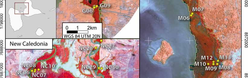
Field experiments were carried out in February, March and May 2014 in Guadeloupe, Mayotte and
New Caledonia, respectively. Forest areas for field sampling were selected from the visual analysis of
satellite images presented in Figure 1 and delineated in situ with the objective of capturing a gradient
of canopy closure within a given study area. The geographic position was recorded using standard
GPS surveys. The resulting sampling areas varied from 25 m2 to 625 m2 relative to the forest stand
structure (i.e., the number and size of trees). The final data set included 10 plots in Guadeloupe,
13 in Mayotte, and 12 in New Caledonia (Table 1). After species identification of each sampled tree,
the diameter at breast height (DBH) was measured, the number of stems per area unit was counted,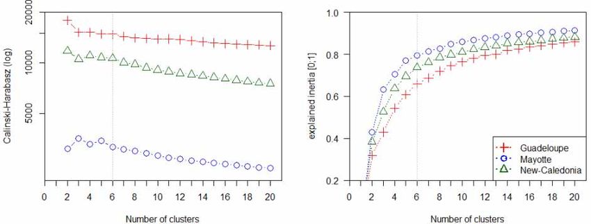
Remote Sens. 2019, 11, 367                                                                                       4 of 17

plot basal area values were computed, and the mean canopy height formed by dominating species
was  evaluated with a hand-held TruePulse® rangefinder.
Remote Sens. 2018, 10, x FOR PEER REVIEW                                                4 of 17

      Figure 1.
      Figure 1. Study
                 Study sites
                       sites and
                             and location
                                 location of
                                          of plots in the
                                                      the three
                                                          three islands
                                                                islands (French Overseas
                                                                                Overseas Territories)
                                                                                         Territories) based
                                                                                                      based on
                                                                                                            on
      Pleiades 1B
      Pleiades  1B images.
                   images.

2.3.
2.2. Hemispherical
     Forest Data Photographs
     Three    series of digital
     Field experiments       were hemispherical     photographs
                                   carried out in February,    March (HP)
                                                                        andwereMay taken
                                                                                    2014 inusing   a GoProMayotte
                                                                                            Guadeloupe,         Hero-3
and
and sensor     sensitivityrespectively.
     New Caledonia,           ranged between
                                           ForestISO   100for
                                                   areas    and   400.
                                                               field      Image were
                                                                      sampling     size was          × 3000
                                                                                              4000from
                                                                                         selected           the pixels.
                                                                                                                  visual
Hemispherical       photographs    were   obtained   with  a  focal  length    of 14 mm   opening
analysis of satellite images presented in Figure 1 and delineated in situ with the objective         at   an  angle ofof
view  of 149.2  ◦ . The shutter speed was adjusted depending on light conditions (between 1/100 and
capturing    a gradient     of canopy closure within a given study area. The geographic position was
1/500s).
recordedAll   photographs
           using     standardwere
                                GPStaken   fromThe
                                     surveys.    the resulting
                                                     forest plotsampling
                                                                 center. Approximatively      15 to25
                                                                              areas varied from     20m²photographs
                                                                                                             to 625 m²
were  taken   for   each  plot with  a one  second   delay  between    each    photo  in order  to have
relative to the forest stand structure (i.e., the number and size of trees). The final data set included   same light 10
exposition  condition    for each photo.  Then  the best photograph     i.e., the photograph   which
plots in Guadeloupe, 13 in Mayotte, and 12 in New Caledonia (Table 1). After species identification    is not  affected
by sunlight
of each       saturation
         sampled            or branches
                      tree, the diametermovement      caused(DBH)
                                           at breast height    by wind washas   been keptthe
                                                                              measured,   and   used for
                                                                                              number     ofanalysis.
                                                                                                             stems per
area The
      unit HP
           wasanalysis
                  counted,consisted
                             plot basalofarea
                                          evaluating   the ratio
                                               values were        betweenand
                                                             computed,        thethe
                                                                                  vegetal
                                                                                     meanand    the free
                                                                                            canopy         skyformed
                                                                                                      height     image
pixels  [48]  using    binarization.    The   Object  Based   Image    Analysis
by dominating species was evaluated with a hand-held TruePulse® rangefinder.       (OBIA)    classification    process
implemented in the eCognition© software was used [49–51]. Each photograph was divided into
several objects. Each object was then classified as sky or vegetation. Objects were determined using
the “Split Contrast” segmentation algorithm, which executes several chessboard segmentations at
different scales before separating the objects into two categories—light and dark—from a threshold
value set after several iterations that maximizes their contrast [52]. The ratio between the number of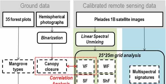
Remote Sens. 2019, 11, 367                                                                                                       5 of 17

pixels classified as “vegetation” and the total number of pixels of the image gave an estimate of the
canopy closure of the forest plot considered.

      Table 1. Ground data with the main forest parameters and canopy closure estimated from hemispherical
      photographs (HP) for all plots in the three sites (G: Guadeloupe; M: Mayotte; NC: New Caledonia).
      The DBH and basal areas represented by “-” are for multi-stem trees. Cluster ID column must be
      interpreted after the reading of the method and result sections. R = Rhizophora sp.; A = Avicennia sp.;
      Lr = Laguncularia racemosa; B = Bruguiera sp.; E = Excoecaria agallocha; Lu = Lumnitzera racemosa;
      Sa = Sonneratia alba; C = Ceriops sp.

                        Stem         Basal       Mean                     Canopy
              DBH                                          Dominating               Vegetation Water        Soil     Shadow     Cluster
   Plot ID.            Density       Area        Height                   Closure
              (cm)                                          Species                 Fraction   Fraction   Fraction   Fraction    ID
                     (Trees.ha−1 ) (m2 .ha−1 )    (m)                   (from HP)
    G02        13        1825          31          4         A+R          0.82        0.68       0.21      0.00       0.09        4
    G04         7        1500           9          3         A+R          0.61        0.64       0.19      0.00       0.14        2
    G05        10        3900          34          6          R           0.82        0.78       0.18      0.00       0.03        2
    G06         7        3700          19          4          Lr          0.54        0.51       0.23      0.02       0.21        4
    G09         9        2100          28          4          R           0.71        0.64       0.26      0.00       0.08        2
    G14         5        3200          13          2          R            0.8        0.78       0.12      0.09       0.00        5
    G15         9        3600          25          7         R+A          0.77        0.80       0.10      0.04       0.04        5
    G19         6        1475           7          4          Lr          0.67        0.65       0.21      0.00       0.13        2
    G20         6        4125          19          4         A+Lr         0.76        0.77       0.08      0.03       0.11        1
    G21        12        2400          34          9         A+R           0.7        0.60       0.16      0.00       0.22        4
    M01         -         300           -           5         Sa          0.26        0.34       0.08      0.23       0.33        5
    M02        23        1400          62          7          R           0.74        0.74       0.00      0.01       0.23        1
    M03        21        1500          90          8         A+R          0.74        0.73       0.00      0.01       0.24        1
    M06         9        4300          51          5        C+B+R         0.72        0.70       0.03      0.12       0.13        3
    M07         4       31,746         45          3        C+B+R         0.77        0.70       0.02      0.06       0.19        3
    M08         4       46,031         57          2          C            0.6        0.48       0.05      0.18       0.27        5
    M09        11        1244          19          4         R+C          0.66        0.57       0.07      0.08       0.26        2
    M10        11         888          11          7        R+B+C         0.58        0.62        0.0      0.03       0.29        2
    M12         3        3100          49          5        R+C+B         0.92        0.93       0.00      0.00       0.06        1
    M13         -         225           -           4         A           0.22        0.24       0.06      0.50       0.18        4
    M14        10        2755          36          4        C+B+R         0.82        0.79       0.02      0.06       0.12        3
    M16        26        1200          64          10         R           0.77        0.71       0.05      0.02       0.19        1
    M17         -         250           -           4         A           0.31        0.39       0.05      0.06       0.48        5
    NC06       20        1000          33          5          R           0.79        0.61       0.00      0.00       0.36        1
    NC07        1       18,400          2          1          A           0.27        0.22       0.01      0.18       0.57        6
    NC08        2        4900           2          1          R           0.38        0.29       0.04      0.14       0.51        3
    NC10        4         825           2           2         R            0.2        0.25       0.01      0.06       0.65        4
    NC16       10        2600          22           3        R+A          0.43        0.39       0.07      0.03       0.49        3
   NC17bis      2       24,000         5            1         A           0.27        0.22       0.05      0.18       0.53        6
   NC17ter      6        1422          4            2         R           0.48        0.35       0.00      0.04       0.59        4
    NC27       18         800          23          6         B+R          0.73        0.70       0.00      0.00       0.29        2
    NC28       13         500           7           6         E           0.68        0.62       0.03      0.01       0.32        1
    NC29        7        1350          16          3          B           0.56        0.40       0.02      0.10       0.46        4
    NC30        6         500           1           3         Lu           0.4        0.35       0.13      0.22       0.29        3
    NC31       12        1400          18           8         R           0.81        0.81       0.12      0.03       0.02        2

2.4. Satellite Image Acquisition and Preprocessing
     Pleiades-1B satellite images were acquired in each study area in a Geotiff format (Table 2) at level
1C. All images were acquired near to high tide time. However, it was difficult to find cloud-free images
with similar viewing and sun angles. We acknowledge that the retrieval of canopy properties can
depend on viewing geometry configurations. For example, acquisition angles can marginally affect
the estimation of canopy closure, which can be overestimated with a high view angle [53], while a
frontward sun-viewing configuration can affect the spectral surface reflectance [54]. To avoid this
problem as much as possible, the images with the smallest angle were favoured, which was not always
possible given the cloud cover and the desired dates of acquisition.
     The intensity of the satellite image pixels was then transformed into radiance values Lλ
(mW.cm2 .sr1 .µm−1 ) using the sensor specific calibration values provided by Airbus Defense and
Space. Then the radiance of each pixel was converted into the top-of-atmosphere (TOA) reflectance ρ
using the following equation (Equation (1)):

                                                                  π.Lλ .D2
                                                          ρλ =                                                                        (1)
                                                                 Esun . cos θs
Remote Sens. 2019, 11, 367                                                                                   6 of 17

where D is the sun-earth distance (expressed in astronomical units), Esun is the corresponding mean
solar exoatmospheric spectral irradiance, and θs is the solar zenithal angle.

      Table 2. Main acquisition parameters of multispectral (MS) Pleiades satellite images. θs and θv are
      the zenithal sun and viewing angles, respectively, while φs-v is the sun-sensor absolute difference
      azimuthal angle.

                                      Bands     Pixel                        High Tide      θs     θv     φs-v
           Site              Sensor                       Acquisition Date
                                      Used      Size                           Time         (◦ )   (◦ )   (◦ )
      Guadeloupe              1B       MS        2m      14 December 2013     2 h before    43      9      25
       Mayotte                1B       MS        2m        18 April 2013       2 h after    33     20     135
     New Caledonia            1B       MS        2m         27 June 2013      1 h before    51     4      149

   Atmospheric corrections were achieved using the FLAASH module process implemented in the
ENVI 5.1®software, this module being based on the MODTRAN radiative transfer model [55].

3. Methods
     As shown in Figure 2, the method consisted of three steps. First, satellite images were analyzed
according to the FCLSU method. Then, vegetation fractions were compared to canopy closure
estimations from analyses of HP through linear regressions. Lastly, the vegetation structure was
mapped    across
Remote Sens.        a k-mean
             2018, 10,         classification
                       x FOR PEER REVIEW      of all fractions resulting from the FCLSU process. 7 of 17

                              Figure 2. Flowchart of data processing in mangrove mapping.
                                                                                 mapping.

3.1.
3.1. Fully
     Fully Constrained
           Constrained Linear
                       Linear Spectral
                               Spectral Unmixing
                                        Unmixing (FCLSU)
                                                    (FCLSU)
      The
      The algorithm
           algorithmprogresses
                       progresses in two  steps:
                                     in two      first, first,
                                              steps:     the endmember     selection,
                                                               the endmember           which consists
                                                                                    selection,  which of selecting
                                                                                                      consists  of
different  pure spectra  representative    of the  different    surfaces  composing     the  image,
selecting different pure spectra representative of the different surfaces composing the image, and  and  then  the
decomposition    of pixel reflectance
then the decomposition                 in order toinquantify
                           of pixel reflectance       order tothe   fractionthe
                                                                 quantify     of fraction
                                                                                  endmembers    within the pixel.
                                                                                           of endmembers   within
the pixel.

3.1.1. Endmember Selection
      Spectral mixture analysis assumes that pixels can be modeled as a linear combination of the
spectral contribution of spectrally pure land cover components called endmembers [33]. To study
the mangrove canopy, the pixel intensity was decomposed into four endmembers: vegetation, water,
soil, and shadow. The spectral satellite multispectral signature of each endmember was derived
Remote Sens. 2019, 11, 367 7 of 17
3.1.1. Endmember Selection
Spectral mixture analysis assumes that pixels can be modeled as a linear combination of the
spectral contribution of spectrally pure land cover components called endmembers [33]. To study
the mangrove canopy, the pixel intensity was decomposed into four endmembers: vegetation, water,
soil, and shadow. The spectral satellite multispectral signature of each endmember was derived
from the average reflectance over more than 10 pixels on MS bands at native spatial resolution (2 m).
The vegetation endmember was obtained over dense mangrove areas showing the highest degrees
of canopy closure, the water spectra were taken from non-turbid water in order to avoid the mixing
with soil spectral properties that occurs with turbid water, and the soil spectra were selected on dry
bare soil in order to avoid the mixing with water that occurs with wet soils. Shadow spectra were
taken from soil surfaces shaded by high mangrove trees and expanded over more than nine pixels [56].
These spectra composed the spectral library used to set the FCLSU algorithm.
3.1.2. Decomposition of Pixel Spectra according to Endmember Spectral Contributions
The decomposition of pixels consisted of evaluating the fractional cover of endmembers of each
pixel according to the following equation (Equation (2)):
n
Rk = ∑ ai Ei,k + ξ k (2)
i
with Rk = pixel reflectance value at k wavelength, ai = abundance of endmember i, Ei,k = reflectance of
endmember i at k wavelength, ξ k = error at k wavelength, and n = number of endmembers.
The results of FCLSU, called "fractions,” are proportional to the contribution of each “endmember”
in the global spectral signature of the pixel. FCLSU takes into account two additional major constraints
(Equation (3)): the sum of the endmember fractions within one pixel must be equal to 1 (sum constraint)
and these fractions must be positive (non-negativity constraint). These constraints enable interpretable
fraction values to be obtained [57].
n
∑ αi = 1
j =1 (3)
with 0 ≤ αi ≤ 1, f or 1 ≤ n ≤ k
and with n = number of endmembers, α = fraction of endmembers i, and k = number of spectral bands.
Applying this algorithm to satellite images with the selected endmembers provided four
images representing vegetation (VF), water (WF), soil (SF), and shadow (ShF) fractions, respectively.
The Sentinel Application Platform software (SNAP v.5.0.0) was used to perform the FCLSU.
3.2. Validation of the FCLSU
A grid composed of 25 m × 25 m polygons was built on unmixed images to fit the swath captured
by hemispherical photographs. Mean values of all fractions were calculated for all polygons of the grid.
In order to validate the model, polygons were selected corresponding to the HP location. Values of
mean VF were then compared with canopy closure estimated from HP. NDVI mean values of polygons
were also compared with canopy closure from HP.
3.3. Vegetation Structure Mapping
The potential of unmixing four components from satellite images of mangroves to characterize
vegetation structure was then analyzed. To do so, a classification applied on the mean fraction values
(fraction classification) was compared with a classification applied on the mean spectral values (spectral
classification) calculated inside all the polygons of the 25 × 25 m grid.of polygons were also compared with canopy closure from HP.
3.3. Vegetation Structure Mapping
The potential of unmixing four components from satellite images of mangroves to characterize
vegetation
Remote structure
Sens. 2019, 11, 367 was then analyzed. To do so, a classification applied on the mean fraction 8 of 17
values (fraction classification) was compared with a classification applied on the mean spectral
values (spectral classification) calculated inside all the polygons of the 25 × 25 m grid.
Both classifications
Both classificationswere performed
were performedwith a 6-cluster
with K-mean
a 6-cluster classification.
K-mean The number
classification. of clusters
The number of
was chosen according to two indices: explained inertia and Calinski-Harabzs index [58]
clusters was chosen according to two indices: explained inertia and Calinski-Harabzs index [58] presented in
Figure 3. in Figure 3.
presented
Figure 3.3. Calinski-Harabasz
Calinski-Harabaszindex
index and
and explained
explained inertia
inertia values
values according
according to different
to different numbernumber of
of cluster.
cluster.
Classifications were then evaluated with confusion matrices built with six photo-interpreted
samples composed ofwere
Classifications one hundred polygons
then evaluated per class.
with The results
confusion are built
matrices presented
withinsix
thephoto-interpreted
following section.
samples composed of one hundred polygons per class. The results are presented in the following
4. Results
section.
4.1. Performance of the FCLSU Approach for Characterizing Mangrove Forest Structures
Average values of the four FCLSU endmembers were compared to canopy closure estimates from
hemispherical photographs and the Normalized Difference Vegetation Index over the 35 forest plots
(Table 1; Figure 4). The FCLSU-derived vegetation fraction was first tested before the potential of the
full decomposition was examined for mangrove forest mapping.
Canopy closure estimates and vegetation fraction values were strongly and linearly correlated
(Figure 4, top left) with R2 = 0.91 (p-value = 2.2 × 10⁻¹⁶ ) over the image dataset and forest plots.
In addition, a Shapiro-Wilk test of normality on residues between the previous relationship and the
extracted values of VF (W = 0.982, p-value = 0.815) showed a normal distribution suggesting that
extreme values did not influence the relationship too significantly. NDVI was poorly correlated
with the vegetation fraction (bottom left) with R2 = 0.34 (Figure 4) and also with the canopy closure
(R2 = 0.29).
Graphs of the regressions showed that the relationship between CC and VF was linear and near
the 1:1 line, regardless of the canopy structure. The relationship between CC and NDVI was near the 1:1
line when the canopy closure reached high values (more than 0.5). The same observation was made for
the VF and NDVI regression line. For open canopies with a low value of CC, the relationship between
CC and NDVI clearly became non-linear and deviated from the 1:1 line. This tends to demonstrate
that the NDVI is dependent on the canopy structure; more precisely, with an open canopy the NDVI is
very inconstant.
The variability of FCLSU vegetation fractions, canopy closure, and NDVI values was analyzed
between and across regional sites (Figure 5). Overall, FCLSU vegetation fractions and canopy closure
exhibited similar variability patterns, distinct from those of the NDVI signatures. Estimates of canopy
closure and vegetation fraction for all plots varied from 0.20 to 0.92 and from 0.24 to 0.93, respectively.
The NDVI responses of mangrove forest plots remained between 0.59 and 0.97. This result suggests a
lack of sensitivity of NDVI but a close match between VF and canopy closure estimates.the 1:1 line, regardless of the canopy structure. The relationship between CC and NDVI was near the
1:1 line when the canopy closure reached high values (more than 0.5). The same observation was
made for the VF and NDVI regression line. For open canopies with a low value of CC, the
relationship between CC and NDVI clearly became non-linear and deviated from the 1:1 line. This
tends to demonstrate that the NDVI is dependent on the canopy structure; more precisely, with an
Remote Sens. 2019, 11, 367 9 of 17
open canopy the NDVI is very inconstant.
Remote Sens. 2018, 10, x FOR PEER REVIEW 10 of 17
The variability of FCLSU vegetation fractions, canopy closure, and NDVI values was analyzed
between and across regional sites (Figure 5). Overall, FCLSU vegetation fractions and canopy
closure exhibited similar variability patterns, distinct from those of the NDVI signatures. Estimates
of canopy closure and vegetation fraction for all plots varied from 0.20 to 0.92 and from 0.24 to 0.93,
respectively. The NDVI responses of mangrove forest plots remained between 0.59 and 0.97. This
result suggests a lack of sensitivity of NDVI but a close match between VF and canopy closure
estimates.
In Guadeloupe, the lowest variation range and the highest mean value were observed of each of
the three parameters considered.
In Mayotte, the VF and canopy closure had close mean values of 0.63 and 0.62, respectively, and
close variation ranges of 0.22 to 0.92 and 0.24 to 0.93, respectively. The NDVI showed a very high
mean value of 0.9 with a tight box plot. The sensitivity of the FCLSU vegetation fraction estimates to
canopy closure was confirmed, as was the irrelevance of NDVI for capturing the variability of
mangrove canopy structure (see the circles in Figure 4, right).
Figure
Figure 4.4. Relationships
In New Relationships
Caledonia, meanbetween
between FCLSU-derived
values vegetation
reached the vegetation
FCLSU-derived fraction
lowest levels values
for both
fraction and canopy
canopy
values and canopy closure
closureclosure
and
estimates
vegetation from
fraction hemispherical
(0.2 and 0.22, photographs
respectively). (left)
The and
mean NDVI
value andvalues
the (right).
height of The
the continuous
NDVI box
estimates from hemispherical photographs (left) and NDVI values (right). The continuous line indicates line
plot
suggest
the besta linear
indicateshigher sensitivity
the best
modellinear thaneach
model
between those observed
between
pair in Guadeloupe
each pair
values. values. and Mayotte.
Figure
Figure 5. Range
5. Range ofofvariations
variations of
of canopy
canopy closure,
closure,VFVF and NDVI
and NDVI values obtained
values from from
obtained the analysis of
the analysis of
Pleiades-1B images acquired over the regional sites. Box plots give the mean, median, quartiles,
Pleiades-1B images acquired over the regional sites. Box plots give the mean, median, quartiles, min min
andand
maxmax values.
values.
4.2. Potential of Fraction Classification for Mapping Mangrove Forest Structures
In Guadeloupe, the lowest variation range and the highest mean value were observed of each of
the threeThe contributions
parameters of the water, shadow and soil fractions were examined as a function of the
considered.
vegetation fraction. Mapping
In Mayotte, the VF and canopy fractions helps in
closure hadunderstanding mangrove
close mean values zonation
of 0.63 and (Figures 6 and 7). and
0.62, respectively,
The classes correspond to different mangrove types interpreted from field data and
close variation ranges of 0.22 to 0.92 and 0.24 to 0.93, respectively. The NDVI showed a very are mainly
high mean
spatially distributed according to a VF intensity gradient.
value of 0.9 with a tight box plot. The sensitivity of the FCLSU vegetation fraction estimates to canopyRemote Sens. 2019, 11, 367 10 of 17
closure was confirmed, as was the irrelevance of NDVI for capturing the variability of mangrove
canopy structure (see the circles in Figure 4, right).
In New Caledonia, mean values reached the lowest levels for both canopy closure and vegetation
fraction (0.2 and 0.22, respectively). The mean value and the height of the NDVI box plot suggest a
higher sensitivity than those observed in Guadeloupe and Mayotte.
4.2. Potential of Fraction Classification for Mapping Mangrove Forest Structures
The contributions of the water, shadow and soil fractions were examined as a function of the
vegetation fraction. Mapping fractions helps in understanding mangrove zonation (Figures 6 and 7).
The classes correspond to different mangrove types interpreted from field data and are mainly spatially
distributed according to a VF intensity gradient.
Mapping of pixel fractions yields vegetation classes that correspond quite closely to different
mangrove structures measured during field campaigns. For the three sites, VF classification is useful
to distinguish dense and canopy closed Rhizophora dominant vegetation from sparse and/or low
Avicennia or Sonneratia open canopy vegetation. Between these two types, a gradient composed of
mixed mangroves shows a decreasing VF from the landward border to the center of the mangrove areas.
On the other hand, some differences can be observed between the sites: for Mayotte and Guadeloupe,
classes 4, 5, and 6 have a low VF and show a high standard deviation, which is not the case in New
Caledonia. This is explained by the composition of mangroves. For example, in Guadeloupe and
Mayotte, polygons of classes 4, 5, and 6 include some pixels covering the crowns of tall and sparse trees
and others covering the gaps between trees. In New Caledonia, classes with a low VF correspond to
homogeneous low Avicennia shrubs with low density foliage and so the variability of the pixel values
is smaller in such a structure than in other territories.
More precisely, in Guadeloupe Island the WF for Avicennia stands is larger than for the other
classes because the trees are sparse and the soil is covered by water during the rainy season (classes 6
and 3). Mixed mangroves dominated by Rhizophora (MIXRHI; class 5) are located in a transition with
other vegetation areas, which explains why they are not very well detected. In Mayotte, the fraction
classification highlights the three types of mangrove: fringe stands composed of Sonneratia alba, inner
mangrove stands dominated by Rhizophora, and landward sparse Avicennia and Ceriops stands located
in the border of tannes. This classification can even distinguish the Bruguiera sp. stand. In New
Caledonia, Rhizophora stands comprised both low, sparse stands and tall, closed stands. This large
gradient generates confusion between all the RHIDOM classes because they are not actually so different
from each other. In fact classes 1 and 2 could be merged as well as classes 3 and 4. Concerning Avicennia,
class 5 is not so different from class 6, which explains why this class is not well detected and is confused
with class 6.
For the three sites, some bias in the classification analyses resulted from a border effect explained
by the size of the polygons (625 m2 ). For fringe stands, like class 6 of Sonneratia in Mayotte,
the encroachment of the polygons on some pixels located on the nearby open-water areas resulted in a
low vegetation fraction and a high water fraction.Remote Sens.Sens.
Remote 2018, 10, x11,
2019, FOR367PEER REVIEW 11 of 17 11 of 17
Figure
Figure 6.
6. K-mean
K-mean classifications
classifications (6
(6 clusters)
clusters) of
of mangrove
mangrove vegetation
vegetation structures based on
structures based on fractions
fractions for
for the
the three
three sites.
sites.Remote Sens. 2019, 11, 367 12 of 17
Remote Sens. 2018, 10, x FOR PEER REVIEW 12 of 17
Figure 7. Component
Figure 7. Component diagrams of of
diagrams the
thefour
fourfractions
fractionsshowing
showing main mangrove vegetation
main mangrove vegetation structures.
structures.Coloured
Colouredpolygons:
polygons:mean
meanfractions
fractions
forfor each
each class.
class. Dotted
Dotted line:line:
standard deviation of the corresponding class. Percentage: user accuracy of the class.
standard deviation of the corresponding class. Percentage: user accuracy of the class.Remote Sens. 2019, 11, 367 13 of 17
4.3. Fraction versus Spectral Classification
In order to validate the fraction classification, a second K-means classification of the grid was
carried out with mean spectral information. The classification results based on the mean values of
spectral bands show an overall accuracy of 38.3% in Guadeloupe, 55% in Mayotte, and 63% in New
Caledonia, while fraction classification shows better accuracies of 78, 73, and 68%, respectively.
However, some classes are better detected with spectral information than with fractions, such
as the AVIDOM class in Guadeloupe, which reaches a user accuracy of 84% (77% with fractions),
the MIXRHI class in Mayotte, which reaches 94.5% accuracy (82% with fractions), and AVIDOM in
New Caledonia, which reaches 88.7% accuracy instead of 49% with fractions. This is explained by the
spectral properties of mangrove species, which play a major role in discriminating mangrove types
when these are composed of different species. This is not the case when the types are composed of the
same species with different patterns of canopy closure. This explains why MIXAVI and AVIDOM can
be clearly detected by fraction classification but not by spectral classification (because both classes are
mainly composed of the same species). It also explains why the fringe stands of Sonneratia alba form
one class with spectral classification and two classes with fraction classification. In New Caledonia,
the RHIDOM mangroves are split into only three classes with spectral classification instead of four
classes with fraction classification, while AVIDOM forms three classes instead of two. So, fraction
classification is globally more adapted to mangrove typology based on species composition than
spectral classification.
Moreover, fractions provide quantitative and standardized information that can be used to create
standard typologies based only on canopy structure such as closed, medium and open mangroves
stands. For example, the closed mangrove can be characterized by vegetation fractions up to 75%, no
matter the location in the world or in the season (that is not the case with NDVI). This represents an
advantage in using standardized typologies for national or international observatories.
5. Discussion and Conclusions
The reliability of FCLSU in monitoring mangrove canopy closure, and its ability to monitor canopy
structure of a broad range of mangrove stands, is demonstrated by the strong correlation (R2 = 0.91)
found between the canopy closure estimated from field hemispherical photographs and vegetation
fraction in image pixels. We also confirmed that NDVI is poorly sensitive to canopy structure in
agreement with a number of previous works [59]. K-means classification of FCLSU-derived fractions
also proved useful for mapping distributional patterns of mangrove zonations.
However, some limitations were encountered during this study. The exploitation of hemispherical
photographs collected in the centre of each plot with lens pointing the sky works well under closed
vegetation. But this HP acquisition approach is to be questioned for low or sparse vegetation.
For low vegetation, HP acquisition could be done by pointing the ground combined with photograph
binarisation applied to discriminate vegetation from soil. For sparse vegetation, the number of
photographs must be adapted to the spatial heterogeneity.
Spectral mixture analysis of satellite images is dependent on solar illumination and viewing angles
as stated in [60]. In New Caledonia, the shadow fraction is observed higher than in the other territories
due probably to the combined effect of canopy gaps and low sun position (high solar zenithal angle)
during the image acquisitions, this resulting in larger shadowed areas. We thus recommend prioritizing
zenithal sun and viewing angles below 20◦ and avoiding grazing sun and hot-spot configurations as
stated in [61] and illustrated through a textural analysis in [62]. Taking care of the flooding level at the
image acquisition time is also crucial for evaluating the soil contribution. We also insist on the need
to carry out physically-based works to interpret scattering mechanisms within forest canopies [63].
Finally, the method developed in this study is specific to mangrove forests characterized by low
understory vegetation which is not the case of tall equatorial mangroves or terrestrial tropical forests
for which interesting research are still to be carried out [64].Remote Sens. 2019, 11, 367 14 of 17
The use of the k-means classification for deriving mangrove classes based on vegetation fractions
appears to be a valuable approach for analyzing and comparing vegetation structure composed of
different species in different regions and distinguishing a broad range of mangrove types. Compared
to a spectral-based classification approach, fraction classification shows higher overall accuracy for the
three sites. This algorithm is also adapted to blind classification of mangrove types across a number
of regions since the use of only six clusters showed good potential in the delineation of mangrove
types, as demonstrated in Figure 6. This component diagram could then act as a learning sample in
the perspective of generalizing classification over larger areas [62]. Moreover, the overall accuracy of
the maps reaching 78% at best may be improved with the support of calibration or validation forest
data derived from LiDAR, stereoscopic, and hyperspectral surveys.
From an ecological perspective, FCLSU advantageously proposes standardized outputs that
can be compared from one site to another. For example, a clear “radial” organization consisting
of Rhizophora stands seaward and Avicennia landward is observed on each of the three study sites.
Very interesting is the sensitivity of our approach that varying vegetation fraction levels among and
between Sonneratia-, Rhizophora-, and Avicennia-dominated stands suggest. This latter point may
prefigure new insights in the assessment of species composition of mangrove stands from satellite
data. The case study of 30–40 m high French Guiana mangroves [65] deserves our future interest for
deeper understanding of FCLSU approach in a vast mangrove region where canopy height and forest
structure develop from seaward to landward in a mosaic of distinct forest stands where Avicennia
compete with Rhizophora species [42].
Measurement of the canopy closure using FCLSU applied to VHSR satellite images may prefigure
future operational monitoring of mangroves over time and yield pivotal data for the assessment of
mangrove resilience to natural or man-induced disturbances.
Author Contributions: Conceptualization: F.T., M.R., F.D. and C.P.; Metholodogy: F.T., M.R., F.D., C.P, F.F. and
D.I.; Field data acquisition: F.T., M.R., F.F., D.I. and C.P.; Writing-review and editing: F.T., M.R. and C.P.
Funding: A part of this study was funded by the French Coastal Conservancy Institute. It was conducted as part
of the PhD work of Florent Taureau supported by the University of Nantes.
Acknowledgments: The authors thank Kildine Veau and Marie Windstein for their help during the field measurements
in the mangroves and Carol Robins for correcting the English of the paper.
Conflicts of Interest: The authors declare no conflict of interest.
References
1. Duke, N.C. Mangrove Coast. In Encyclopedia of Marine Geosciences; Harff, J., Meschede, M., Petersen, S.,
Thiede, J., Eds.; Springer: Berlin, Germany, 2014; pp. 1–17.
2. Feller, I.C.; Lovelock, C.E.; Berger, U.; McKee, K.L.; Joye, S.B.; Ball, M.C. Biocomplexity in Mangrove
Ecosystems. Annu. Rev. Mar. Sci. 2010, 2, 395–417. [CrossRef] [PubMed]
3. Krauss, K.W.; Lovelock, C.E.; McKee, K.L.; López-Hoffman, L.; Ewe, S.M.; Sousa, W.P. Environmental drivers
in mangrove establishment and early development: A review. Aquat. Bot. 2008, 89, 105–127. [CrossRef]
4. Chapman, V.J. Mangrove Vegetation; Cramer: Vaduz, Liechtenstein, 1976.
5. Friess, D.A.; Lee, S.Y.; Primavera, J.H. Turning the tide on mangrove loss. Mar. Pollut. Bull. 2016, 109,
673–675. [CrossRef] [PubMed]
6. Alongi, D.M. Mangrove forests: Resilience, protection from tsunamis, and responses to global climate change.
Estuar. Coast. Shelf Sci. 2008, 76, 1–13. [CrossRef]
7. Bouillon, S.; Borges, A.V.; Castañeda-Moya, E.; Diele, K.; Dittmar, T.; Duke, N.C.; Kristensen, E.; Lee, S.Y.;
Marchand, C.; Rivera-Monroy, V.H.; et al. Mangrove production and carbon sinks: A revision of global
budget estimates: Global mangrove carbon budgets. Glob. Biogeochem. Cycles 2008, 22. [CrossRef]
8. Donato, D.C.; Kauffman, J.B.; Murdiyarso, D.; Kurnianto, S.; Stidham, M.; Kanninen, M. Mangroves among
the most carbon-rich forests in the tropics. Nat. Geosci. 2011, 4, 293–297. [CrossRef]Remote Sens. 2019, 11, 367 15 of 17
9. Duke, N.C.; Nagelkerken, I.; Agardy, T.; Wells, S.; van Bochove, J.-W. The Importance of Mangroves to People: A
Call to Action; United Nations Environment Programme World Conservation Monitoring Centre: Cambridge,
UK, 2014.
10. De Lacerda, L.D. Mangrove Ecosystems: Function and Management; Springer: Berlin, Germany, 2010.
11. Lee, S.Y.; Primavera, J.H.; Dahdouh-Guebas, F.; McKee, K.; Bosire, J.O.; Cannicci, S.; Diele, K.; Fromard, F.;
Koedam, N. Cyril Marchand Ecological role and services of tropical mangrove ecosystems: a reassessment:
Reassessment of mangrove ecosystem services. Glob. Ecol. Biogeogr. 2014, 23, 726–743. [CrossRef]
12. Spalding, M.; Kainuma, M.; Collins, L. World Atlas of Mangroves; Routledge: Abingdon, UK, 2010.
13. Food and Agriculture Organization of the United Nations (FAO). The World’s Mangroves 1980–2005: A
Thematic Study Prepared in the Framework of the Global Forest Resources Assessment 2005; Food and Agriculture
Organization of the United Nations: Rome, Italy, 2007.
14. Ellison, J.C. Vulnerability assessment of mangroves to climate change and sea-level rise impacts.
Wetl. Ecol. Manag. 2015, 23, 115–137. [CrossRef]
15. Ellison, J.; Zouh, I. Vulnerability to Climate Change of Mangroves: Assessment from Cameroon, Central
Africa. Biology 2012, 1, 617–638. [CrossRef]
16. Gilman, E.L.; Ellison, J.; Duke, N.C.; Field, C. Threats to mangroves from climate change and adaptation
options: A review. Aquat. Bot. 2008, 89, 237–250. [CrossRef]
17. Li, S.; Meng, X.; Ge, Z.; Zhang, L. Evaluation of the threat from sea-level rise to the mangrove ecosystems in
Tieshangang Bay, Southern China. Ocean Coast. Manag. 2015, 109, 1–8. [CrossRef]
18. Alongi, D.M. Present state and future of the world’s mangrove forests. Environ. Conserv. 2002, 29, 331–349.
[CrossRef]
19. Panta, M. Analisys of Forest Canopy Density and Factors Affecting It Using RS and GIS Techniques—A Case Study
from Chitwan District of Nepal; International Institue for Geo-Information Science and Earth Observation:
Hengelosestraat, The Netherlands, 2003.
20. Birnbaum, P. Canopy surface topography in a French Guiana forest and the folded forest theory. Plant Ecol.
2001, 153, 293–300. [CrossRef]
21. Lowman, M.D.; Schowalter, T.; Franklin, J. Methods in Forest Canopy Research; University of California Press:
Berkeley, CA, USA, 2012.
22. Parker, G.G. Structure and microclimate of forest canopies. In Forest Canopies: A Review of Research on a
Biological Frontier; Lowman, M., Nadkarni, N., Eds.; Academic Press: San Diego, CA, USA, 1995; pp. 73–106.
23. Frazer, G.W.; Trofymow, J.A.; Lertzman, K.P. A Method for Estimating Canopy Openness, Effective Leaf Area
Index, and Photosynthetically Active Photon Flux Density Using Hemispherical Photography and Computerized
Image Analysis Techniques; Canadian Forest Service, Pacific Forestry Centre: Victoria, BC, Canada, 1997.
24. Smith, M.-L.; Anderson, J.; Fladeland, M. Forest canopy structural properties. In Field Measurements for Forest
Carbon Monitoring: A Landscape-Scale Approach; Springer: Berlin, Germany, 2008; pp. 179–196.
25. Green, E.P.; Clark, C.D.; Mumby, P.J.; Edwards, A.J.; Ellis, A.C. Remote sensing techniques for mangrove
mapping. Int. J. Remote Sens. 1998, 19, 935–956. [CrossRef]
26. Sari, S.P.; Rosalina, D. Mapping and Monitoring of Mangrove Density Changes on tin Mining Area.
Procedia Environ. Sci. 2016, 33, 436–442. [CrossRef]
27. Yuvaraj, E.; Dharanirajan, K.; Saravanan, N.; Karpoorasundarapandian, N. Evaluation of Vegetation Density of
the Mangrove Forest in South Andaman Island Using Remote Sensing and GIS Techniques; International Science
Congress Association: India, 2014; pp. 19–25.
28. Garcia-Haro, F.J.; Gilabert, M.A.; Melia, J. Linear spectral mixture modelling to estimate vegetation amount
from optical spectral data. Int. J. Remote Sens. 1996, 17, 3373–3400. [CrossRef]
29. Braun, M.; Martin, H. Mapping imperviousness using NDVI and linear spectral unmixing of ASTER data in
the Cologne-Bonn region (Germany). In Proceedings of the SPIE 10th International Symposium on Remote
Sensing, Barcelona, Spain, 8–12 September 2003.
30. Drake, N.A.; Mackin, S.; Settle, J.J. Mapping Vegetation, Soils, and Geology in Semiarid Shrublands Using
Spectral Matching and Mixture Modeling of SWIR AVIRIS Imagery. Remote Sens. Environ. 1999, 68, 12–25.
[CrossRef]Remote Sens. 2019, 11, 367 16 of 17
31. Guerschman, J.P.; Scarth, P.F.; McVicar, T.R.; Renzullo, L.J.; Malthus, T.J.; Stewart, J.B.; Rickards, J.E.;
Trevithick, R. Assessing the effects of site heterogeneity and soil properties when unmixing photosynthetic
vegetation, non-photosynthetic vegetation and bare soil fractions from Landsat and MODIS data. Remote Sens.
Environ. 2015, 161, 12–26. [CrossRef]
32. Stagakis, S.; Vanikiotis, T.; Sykioti, O. Estimating forest species abundance through linear unmixing of
CHRIS/PROBA imagery. ISPRS J. Photogramm. Remote Sens. 2016, 119, 79–89. [CrossRef]
33. Liu, T.; Yang, X. Mapping vegetation in an urban area with stratified classification and multiple endmember
spectral mixture analysis. Remote Sens. Environ. 2013, 133, 251–264. [CrossRef]
34. Silvan-Cardenas, J.L.; Wang, L. Fully Constrained Linear Spectral Unmixing: Analytic Solution Using Fuzzy
Sets. IEEE Trans. Geosci. Remote Sens. 2010, 48, 3992–4002.
35. Souza, C. Mapping forest degradation in the Eastern Amazon from SPOT 4 through spectral mixture models.
Remote Sens. Environ. 2003, 87, 494–506. [CrossRef]
36. Ji, M.; Feng, J. Subpixel measurement of mangrove canopy closure via spectral mixture analysis.
Front. Earth Sci. 2011, 5, 130–137. [CrossRef]
37. Tiner, R.W.; Lang, M.W.; Klemas, V.V. Remote Sensing of Wetlands: Applications and Advances; CRC Press:
Boca Raton, FL, USA, 2015.
38. Haase, D.; Jänicke, C.; Wellmann, T. Front and back yard green analysis with subpixel vegetation fractions
from earth observation data in a city. Landsc. Urban Plan. 2019, 182, 44–54. [CrossRef]
39. Dronova, I. Object-Based Image Analysis in Wetland Research: A Review. Remote Sens. 2015, 7, 6380–6413.
[CrossRef]
40. Fei, S.X.; Shan, C.H.; Hua, G.Z. Remote Sensing of Mangrove Wetlands Identification. Procedia Environ. Sci.
2011, 10, 2287–2293. [CrossRef]
41. Heumann, B.W. Satellite remote sensing of mangrove forests: Recent advances and future opportunities.
Prog. Phys. Geogr. 2011, 35, 87–108. [CrossRef]
42. Proisy, C.; Couteron, P.; Fromard, F. Predicting and mapping mangrove biomass from canopy grain analysis
using Fourier-based textural ordination of IKONOS images. Remote Sens. Environ. 2007, 109, 379–392.
[CrossRef]
43. Imbert, D.; Labbé, P.; Rousteau, A. Hurricane damage and forest structure in Guadeloupe, French West
Indies. J. Trop. Ecol. 1996, 12, 663–680. [CrossRef]
44. Herteman, M.; Fromard, F.; Lambs, L. Effects of pretreated domestic wastewater supplies on leaf pigment
content, photosynthesis rate and growth of mangrove trees: A field study from Mayotte Island, SW Indian
Ocean. Ecol. Eng. 2011, 37, 1283–1291. [CrossRef]
45. Cremades, C. Cartographie des Habitats Naturels des Mangroves de Mayotte; Direction de l’Agriculture et de la
Forêt Service Environnement et Forêt: Mamoudzou, Mayotte, 2010.
46. Jeanson, M. Morphodynamique du Littoral de Mayotte: des Processus au Réseau de Surveillance; Université du
Littoral Côte d’Opale: Dunkerque, France, 2009.
47. Marchand, C.; Dumas, P. Typologies et Biodiversité des Mangroves de Nouvelle-Calédonie; IRD: Nouméa,
Nouvelle-Calédonie, 2007.
48. Glatthorn, J.; Beckschäfer, P. Standardizing the Protocol for Hemispherical Photographs: Accuracy Assessment of
Binarization Algorithms. PLoS ONE 2014, 9, e111924. [CrossRef] [PubMed]
49. Betbeder, J.; Nabucet, J.; Pottier, E.; Baudry, J.; Corgne, S.; Hubert-Moy, L. Detection and Characterization of
Hedgerows Using TerraSAR-X Imagery. Remote Sens. 2014, 6, 3752–3769. [CrossRef]
50. Betbeder, J.; Hubert-Moy, L.; Burel, F.; Corgne, S.; Baudry, J. Assessing ecological habitat structure from local
to landscape scales using synthetic aperture radar. Ecol. Indic. 2015, 52, 545–557. [CrossRef]
51. Betbeder, J.; Rapinel, S.; Corgne, S.; Pottier, E.; Hubert-Moy, L. TerraSAR-X dual-pol time-series for mapping
of wetland vegetation. ISPRS J. Photogramm. Remote Sens. 2015, 107, 90–98. [CrossRef]
52. Reference Book, eCognition Developer 8.9’; Trimble: Sunnyvale, CA, USA, 2013.
53. Lobell, D.B.; Asner, G.P.; Law, B.E.; Treuhaft, R.N. View angle effects on canopy reflectance and spectral
mixture analysis of coniferous forests using AVIRIS. Int. J. Remote Sens. 2002, 23, 2247–2262. [CrossRef]
54. Viennois, G.; Proisy, C.; Feret, J.B.; Prosperi, J.; Sidik, F.; Suhardjono; Rahmania, R.; Longépé, N.; Germain, O.;
Gaspar, P. Multitemporal Analysis of High-Spatial-Resolution Optical Satellite Imagery for Mangrove Species
Mapping in Bali, Indonesia. IEEE J. Sel. Top. Appl. Earth Obs. Remote Sens. 2016, 9, 3680–3686. [CrossRef]Remote Sens. 2019, 11, 367 17 of 17
55. Adler-Golden, S.M.; Matthew, M.W.; Bernstein, L.S.; Levine, R.Y.; Berk, A.; Richtsmeier, S.C.; Acharya, P.K.;
Anderson, G.P.; Felde, J.W.; Hoke, M.L.; et al. Atmospheric Correction for Short-wave Spectral Imagery
Based on MODTRAN4. Soc. Photo-Opt. Instrum. Eng. 1999, 3753, 61–70.
56. Adeline, K.R.M.; Chen, M.; Briottet, X.; Pang, S.K.; Paparoditis, N. Shadow detection in very high spatial
resolution aerial images: A comparative study. ISPRS J. Photogramm. Remote Sens. 2013, 80, 21–38. [CrossRef]
57. Heinz, D.C. Fully constrained least squares linear spectral mixture analysis method for material quantification
in hyperspectral imagery. IEEE Trans. Geosci. Remote Sens. 2001, 39, 529–545. [CrossRef]
58. Caliński, T.; Harabasz, J. A dendrite method for cluster analysis. Commun. Stat. 1974, 3, 1–27.
59. Asner, G.P.; Warner, A.S. Canopy shadow in IKONOS satellite observations of tropical forests and savannas.
Remote Sens. Environ. 2003, 87, 521–533. [CrossRef]
60. Dennison, P.E.; Halligan, K.Q.; Roberts, D.A. A comparison of error metrics and constraints for multiple
endmember spectral mixture analysis and spectral angle mapper. Remote Sens. Environ. 2004, 93, 359–367.
[CrossRef]
61. Kuusk, A. The Hot Spot Effect in Plant Canopy Reflectance. In Photon-Vegetation Interactions: Applications in
Optical Remote Sensing and Plant Ecology; Myneni, R.B., Ross, J., Eds.; Springer: Berlin/Heidelberg, Germany,
1991; pp. 139–159.
62. Barbier, N.; Proisy, C.; Véga, C.; Sabatier, D.; Couteron, P. Bidirectional texture function of high resolution
optical images of tropical forest: An approach using LiDAR hillshade simulations. Remote Sens. Environ.
2011, 115, 167–179. [CrossRef]
63. Fromard, F.; Vega, C.; Proisy, C. Half a century of dynamic coastal change affecting mangrove shorelines of
French Guiana. A case study based on remote sensing data analyses and field surveys. Mar. Geol. 2004, 208,
265–280. [CrossRef]
64. Ozdemir, I. Linear transformation to minimize the effects of variability in understory to estimate percent
tree canopy cover using RapidEye data. GIS Remote Sens. 2014, 51, 288–300. [CrossRef]
65. Proisy, C.; Féret, J.B.; Lauret, N.; Gastellu-Etchegorry, J.P. Mangrove Forest Dynamics Using Very High
Spatial Resolution Optical Remote Sensing A2—Baghdadi, Nicolas. In Land Surface Remote Sensing in Urban
and Coastal Areas; Zribi, M., Ed.; Elsevier: Amsterdam, The Netherlands, 2016; pp. 269–295.
© 2019 by the authors. Licensee MDPI, Basel, Switzerland. This article is an open access
article distributed under the terms and conditions of the Creative Commons Attribution
(CC BY) license (http://creativecommons.org/licenses/by/4.0/).You can also read