Monitoring pigment-driven vegetation changes in a low-Arctic tundra ecosystem using digital cameras - GFZpublic
←
→
Page content transcription
If your browser does not render page correctly, please read the page content below
Monitoring pigment-driven vegetation changes in a low-Arctic
             tundra ecosystem using digital cameras
 ALISON L. BEAMISH,1, NICHOLAS C. COOPS,2 TXOMIN HERMOSILLA,2 SABINE CHABRILLAT,3 AND BIRGIT HEIM1
                  1
                    Alfred Wegener Institute, Periglacial Research, Telegrafenberg A45, 14473 Potsdam, Germany
          2
           Integrated Remote Sensing Studio (IRSS), Faculty of Forestry, University of British Columbia, 2424 Main Mall,
                                           Vancouver, British Columbia V6T1Z4 Canada
     3
       Helmholtz Centre Potsdam (GFZ), German Research Centre for Geosciences, Telegrafenberg A17, 14473 Potsdam, Germany

  Citation: Beamish, A. L., N. C. Coops, T. Hermosilla, S. Chabrillat, and B. Heim. 2018. Monitoring pigment-driven
  vegetation changes in a low-Arctic tundra ecosystem using digital cameras. Ecosphere 9(2):e02123. 10.1002/ecs2.2123

  Abstract. Arctic vegetation phenology is a sensitive indicator of a changing climate, and rapid assess-
  ment of vegetation status is necessary to more comprehensively understand the impacts on foliar condition
  and photosynthetic activity. Airborne and space-borne optical remote sensing has been successfully used
  to monitor vegetation phenology in Arctic ecosystems by exploiting the biophysical and biochemical
  changes associated with vegetation growth and senescence. However, persistent cloud cover and low sun
  angles in the region make the acquisition of high-quality temporal optical data within one growing season
  challenging. In the following study, we examine the capability of “near-field” remote sensing technologies,
  in this case digital, true-color cameras to produce surrogate in situ spectral data to characterize changes in
  vegetation driven by seasonal pigment dynamics. Simple linear regression was used to investigate relation-
  ships between common pigment-driven spectral indices calculated from field-based spectrometry and red,
  green, and blue (RGB) indices from corresponding digital photographs in three dominant vegetation com-
  munities across three major seasons at Toolik Lake, North Slope, Alaska. We chose the strongest and most
  consistent RGB index across all communities to represent each spectral index. Next, linear regressions were
  used to relate RGB indices and extracted leaf-level pigment content with a simple additive error propaga-
  tion of the root mean square error. Results indicate that the green-based RGB indices had the strongest rela-
  tionship with chlorophyll a and total chlorophyll, while a red-based RGB index showed moderate
  relationships with the chlorophyll to carotenoid ratio. The results suggest that vegetation color contributes
  strongly to the response of pigment-driven spectral indices and RGB data can act as a surrogate to track
  seasonal vegetation change associated with pigment development and degradation. Overall, we find that
  low-cost, easy-to-use digital cameras can monitor vegetation status and changes related to seasonal foliar
  condition and photosynthetic activity in three dominant, low-Arctic vegetation communities.

  Key words: hyperspectral; low-Arctic; red, green, and blue indices; true-color digital photography; vegetation
  pigments.

  Received 20 January 2018; accepted 24 January 2018. Corresponding Editor: Debra P. C. Peters.
  Copyright: © 2018 Beamish et al. This is an open access article under the terms of the Creative Commons Attribution
  License, which permits use, distribution and reproduction in any medium, provided the original work is properly cited.
    E-mail: abeamish@awi.de

INTRODUCTION                                                      feedbacks (Zhang et al. 2007, Bhatt et al. 2010,
                                                                  Parmentier and Christensen 2013). Climatic
  Changes to the functioning of Arctic ecosys-                    changes have been accompanied by broad-scale
tems, such as shifts in photosynthetic activity, net              shifts in Arctic vegetation community composi-
primary productivity, and species composition                     tion and species distribution, as well as fine-scale
influence global climate change and the resulting                  shifts in individual plant reproduction and

                ❖ www.esajournals.org                         1             February 2018   ❖ Volume 9(2) ❖ Article e02123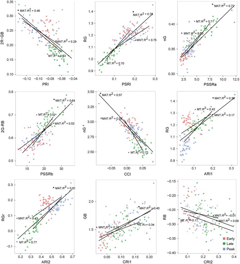
BEAMISH ET AL.

phenology (Walker et al. 2006, Bhatt et al. 2010,         activity and foliar condition at key phenological
Elmendorf et al. 2012a, Bjorkman et al. 2015, Pre-        phases of Arctic vegetation.
vey et al. 2017). Changes in vegetation phenol-             The major photosynthetic pigment groups of
ogy can impact overall ecosystem functioning as           chlorophyll and carotenoids absorb strongly in
a result of mismatched species–climate interac-           the visible spectrum creating unique spectral sig-
tions. This in turn can impact species photosyn-          natures (Curran 1989, Gitelson and Merzlyak
thetic activity and growth through increased              1998, Gitelson et al. 2002, Coops et al. 2003).
vulnerability to events such as frost, soil satura-       Chlorophyll pigments are the dominant factor
tion, or disruption to species chilling require-          controlling the amount of light absorbed by a
ments (Inouye and McGuire 1991, Yu et al. 2010,           plant and therefore photosynthetic potential,
Cook and Wolkovich 2012, Høye et al. 2013,                which ultimately dictates primary productivity.
Wheeler et al. 2015).                                     Carotenoids (carotenes and xanthophylls) are
   In Arctic ecosystems, snow pack conditions             responsible for absorbing incident radiation and
and timing of snowmelt, rather than temperature,          providing energy to the photosynthetic process
are primary drivers of the onset of vegetation phe-       and are often used to provide information on the
nology (Billings and Bliss 1959, Bjorkman et al.          physiological status of vegetation (Young and
2015). Changing snowmelt dynamics due to                  Britton 1990, Bartley and Scolnik 1995). The third
changes in winter precipitation and spring tem-           major pigment group of anthocyanins (water-
peratures have been shown to directly influence            soluble flavonoids) has a less concise function in
tundra vegetation phenology throughout the                vegetation providing photoprotection (Steyn
growing season (Bjorkman et al. 2015). Thus, the          et al. 2002, Close and Beadle 2003), drought and
onset of the growing season, or the leaf-out stage,       freezing protection (Chalker-Scott 1999), and
acts as a benchmark of phenology, and identifica-          they have been shown to play a role in recovery
tion and characterization of this stage are key to        from foliar damage (Gould et al. 2002). Photo-
understanding the overall and subsequent phe-             synthetic pigments influence a wide range of
nology and fitness of tundra vegetation (Iler et al.       plant functioning from photosynthetic efficiency
2013, Wheeler et al. 2015). The timing of maxi-           to protective functions (Demmig-Adams and
mum expansion and elongation of leaves and                Adams 1996) and can be measured destructively
stems and when vegetation is at, or near, peak            through laboratory analysis or non-destructively
photosynthetic activity, or peak greenness, are           using high spectral resolution remote sensing
also important benchmarks of phenological                 (Gitelson et al. 1996, 2001, 2002, 2006).
phases. Peak greenness marks the climax of the               The development and degradation of chloro-
growing season, the timing and magnitude of               phyll pigments as a result of vegetation emer-
which can indicate ecosystem functioning, and             gence, stress, or senescence causes a distinct shift
acts as a benchmark for long-term monitoring of           in spectral signatures in the visible spectrum to
tundra productivity (Bhatt et al. 2010, 2013). A          shorter wavelengths due to a narrowing of the
final benchmark of phenological phase is the end           major chlorophyll absorption feature (550–
of the growing season, or senescence. In combina-         750 nm) and an overall reduction in spectral
tion with leaf-out, senescence dictates growing           absorption (Ustin and Curtiss 1990). Carotenoids
season length and has implications for overall sea-       (yellow to orange) and anthocyanins (blue to red)
sonal productivity and carbon assimilation (Park          have less straightforward seasonal, and therefore
et al. 2016). Characterizing key biophysical prop-        spectral, shifts. The spectral absorption by carote-
erties of Arctic vegetation associated with these         noid pigments can result in mixed or masked
three benchmark phenological phases is impor-             spectral absorption with chlorophyll signals due
tant for accurate monitoring and quantification of         to overlapping absorption features in the visible
local and regional changes in Arctic vegetation           spectrum (400–700 nm). Carotenoids and antho-
and in turn Arctic and global changes to energy           cyanins often have relatively higher concentra-
and carbon cycling, as well as associated feed-           tions in senesced and young leaves when
backs. The presence and seasonal changes in veg-          chlorophyll concentrations are relatively low
etation pigment content can be used to infer              (Tieszen 1972, Sims and Gamon 2002, Stylinski
biophysical properties including photosynthetic           et al. 2002). However, in general, the predictable

              ❖ www.esajournals.org                   2            February 2018   ❖ Volume 9(2) ❖ Article e02123
BEAMISH ET AL.
and distinct spectral features created by changes consumer-grade digital cameras have extremely
in vegetation pigment content allow inferences of high spatial resolution and high data collection
ecological parameters such as photosynthetic capabilities and are less weather dependent than
activity, nutrient concentration, and biomass airborne and optical satellite remote sensing as
(Mutanga and Prins 2004, Mutanga and Skidmore varying illumination can be easily corrected
2004, Asner and Martin 2008, Ustin et al. 2009). (Richardson et al. 2007, Nijland et al. 2014).
Of particular interest for in situ and laboratory Large-scale, true-color, repeatable digital photog-
spectroscopy of vegetation and phenology are the raphy networks in temperate ecosystems such as
spectral characterization of the xanthophyll cycle the PhenoCam network (http://phenocam.sr.
(carotenoids) and the ratio between photosynthetic unh.edu/webcam/) highlight the existing ecologi-
pigments of carotenoids and chlorophyll as they cal applications of this method. Additional work
relate to radiation use efficiency and in turn radia- by Richardson et al. (2007) and Coops et al. (2012)
tive transfer models (Blackburn 2007, Garbulsky demonstrates the link between ground-based
et al. 2011, Gamon et al. 2016). Radiative transfer true-color camera systems and satellite-scale
models are used to simulate leaf and canopy spec- (Landsat and MODIS) observations. In addition
tral reflectance and transmittance, and have been to phenological parameters, well-established RGB
the basis for the inverse determination of biophysi- indices derived from consumer-grade digital
cal and biochemical parameters of vegetation cameras have been shown to accurately identify
based on spectral reflectance (Feret et al. 2011). vegetation cover in Arctic tundra and temperate
Even at lower spectral resolution, the importance forests (Richardson et al. 2007, Ide and Oguma
of pigments and pigment dynamics related to the 2010, Nijland et al. 2014, Beamish et al. 2016) and
xanthophyll cycle can be seen in available products can be closely related to gross primary production
for recent satellite missions; for example, the Euro- in grasslands, temperate forests, Arctic tundra,
pean Space Agency’s (ESA) Sentinel-2 provides and wetlands (Ahrends et al. 2009, Migliavacca
many pigment-driven vegetation indices (see et al. 2011, Westergaard-Nielsen et al. 2013,
https://www.sentinel-hub.com/develop/documenta Anderson et al. 2016), as well as containing a sen-
tion/eo_products/Sentinel2EOproducts). sitivity to changes in plant photosynthetic pig-
While highly valuable, in situ reflectance spec- ments (Ide and Oguma 2013).
troscopy, like optical remote sensing, is challeng- In this study, we examine the capability of
ing for remote Arctic field sites. Remote locations, in situ, true-color digital photography to act as a
challenges associated with field-based monitor- surrogate for in situ spectral data in assessing pig-
ing, and atmospheric and illumination conditions ment-driven vegetation changes associated with
of optical satellite imagery of these areas limit three key seasons representing early, peak, and
available optical data, hindering phenological late season, in three dominant, low-Arctic tundra
studies. To complement the use of airborne and vegetation communities. To do this, we asked the
satellite imagery to measure vegetation pigments following research questions: (1) What are the
and classify biophysical properties in Arctic relationships between RGB indices and in situ,
ecosystems, the use of true-color digital photogra- pigment-driven spectral indices? (2) How do
phy and red, green, and blue (RGB) indices to these relationships change with community type
infer photosynthetic activity and foliar condition and season? (3) To what extent do the indices rep-
is a promising area of study and should be exam- resent actual chlorophyll and carotenoid content?
ined (Anderson et al. 2016, Beamish et al. 2016). We conclude with proposing the RGB indices best
Research has shown that Arctic vegetation suited as proxies for in situ spectral data for moni-
changes are complex with strong site and species- toring seasonal vegetation change and the related
specific responses through space and time pigment dynamics in a low-Arctic tundra.
(Walker et al. 2006, Bhatt et al. 2010, Elmendorf
et al. 2012b, Bjorkman et al. 2015, Prevey et al. METHODS
2017). True-color digital photography represents
both a simple and cost-effective way to increase Study site
data volume both spatially and temporally to cap- Data were collected at the Toolik Field Station
ture site and species-specific responses. Data from (68°62.570 N, 149°61.430 W) on the North Slope of
❖ www.esajournals.org 3 February 2018 ❖ Volume 9(2) ❖ Article e02123BEAMISH ET AL.
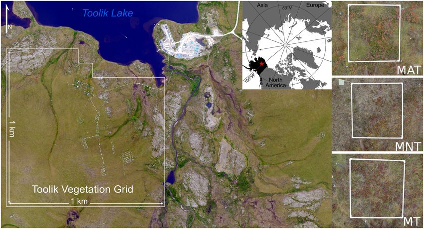
Fig. 1. Toolik Vegetation Grid located in the Toolik Research Area on the North Slope of the Brooks Range in
northern Alaska and a late season example plots of the three vegetation communities monitored in the study.
MAT, moist acidic tussock tundra; MNT, moist non-acidic tundra; MT, moss tundra.
the Brooks Range, in north central Alaska in the within the Long-term Toolik Vegetation Grid are
growing season of 2016. The Toolik Area is repre- shown in Table 1.
sentative of the southern Arctic Foothills, a phys-
iographic province of the North Slope (Walker Digital photographs
et al. 1989). Vegetation is a combination of moist In order to capture the three major seasons of
tussock tundra, wet sedge meadows, and dry early, peak, and late, we acquired true-color digi-
upland heaths. Data were acquired in the Toolik tal photographs on three days in the 2016 grow-
Vegetation Grid, a 1 9 1 km long-term monitor- ing season (June 16, day of year [DOY] 165; July
ing site established by the National Science Foun- 11, DOY 192; August 17, DOY 229). Images were
dation (NSF) as part of the Department of taken at nadir approximately 1 m off the ground
Energy’s R4D (Response, Resistance, Resilience, with a white 1 9 1 m frame for registration of
and Recovery to Disturbance in Arctic Ecosys- off nadir images (Fig. 1). According to the Toolik
tems) project (Fig. 1). Vegetation monitoring Lake Environmental Data Centre (https://toolik.
plots (1 9 1 m) are positioned in close proximity alaska.edu/edc/, 2017) phenology record that
to equally spaced site markers delineating the monitors 15 dominant species at the Toolik Field
intersection of the Universal Transverse Mercator Station, the first image acquisition date occurred
(UTM) coordinates and each point within the two weeks after the average date of first leaf-out
grid. A subset of the grid was sampled for the (May 29, DOY 149) accurately capturing the peak
purpose of this study representing three distinct of the early leaf-out phase. The second acquisi-
and dominant vegetation communities as tion took place one week after average date of
defined by Bratsch et al. (2016) (Fig. 1). The com- last flower petal drop (July 3, DOY 185) and
munities include moist acidic tundra (MAT), within one week of recorded full green-up (end
moist non-acidic tundra (MNT), and moss tun- of June). The final acquisition took place three
dra (MT). A detailed description and representa- weeks after average first day of fall color change
tiveness (% cover of the Toolik Vegetation Grid) (July 27, DOY 209) and within the range of
of the three vegetation communities sampled recorded peak fall colors (mid-August).
❖ www.esajournals.org 4 February 2018 ❖ Volume 9(2) ❖ Article e02123BEAMISH ET AL.
Table 1. Description of the three vegetation communities monitored in this study.
Community Description Detailed description % cover
Moist acidic Occurs on soils with pH < 5.0–5.5 Betula nana–Eriophorum vaginatum. Dwarf-shrub, sedge, 6.1
tussock and is dominated by dwarf erect moss tundra (shrubby tussock tundra dominated by
tundra shrubs such as Betula nana and dwarf birch, Betula nana). Mesic to subhygric, acidic,
Salix pulchra, graminoids species moderate snow. Lower slopes and water-track margins.
(Eriophorum vaginatum), and Mostly on Itkillik I glacial surfaces
acidophilous mosses Salix pulchra–Carex bigelowii. Dwarf-shrub, sedge, moss
tundra (shrubby tussock tundra dominated by diamond-
leaf willow, Salix pulchra). Subhygric, moderate snow,
lower slopes with solifluction
Moist Dominated by mosses, Carex bigelowii–Dryas integrifolia, typical subtype; 5.8
non-acidic graminoids (Carex bigelowii), and Tomentypnum nitens–Carex bigelowii, Salix glauca subtype:
tundra prostrate dwarf shrubs (Dryas nontussock sedge, dwarf-shrub, moss tundra (moist
integrifolia) non-acidic tundra). Mesic to subhygric, non-acidic
(pH > 5.5), shallow to moderate snow. Solifluction areas
and somewhat unstable slopes. Some south-facing slopes
have scattered glaucous willow (Salix glauca)
Mossy A moist acidic tussock tundra- Eriophorum vaginatum–Sphagnum; Carex bigelowii– 54.2
tussock type community dominated by Sphagnum: tussock sedge, dwarf-shrub, moss tundra
tundra sedges (E. vaginatum) and (tussock tundra, moist acidic tundra). Mesic to
abundant Sphagnum spp. subhygric, acidic, shallow to moderate snow, stable. This
unit is the zonal vegetation on fine-grained substrates
with ice-rich permafrost. Some areas on steeper slopes
with solifluction are dominated by Bigelow sedge
(Carex bigelowii)
Images were acquired with a consumer-grade Digital camera indices 2G-RB and nG have
digital camera (Panasonic DM3 LMX, Osaka, been used to monitor vegetation phenology and
Japan) in raw format, between 10:00 h and biomass extensively (Richardson et al. 2007, Ide
14:00 h, under uniform cloud cover to reduce the and Oguma 2013, Beamish et al. 2016). Addition-
influence of shadow and illumination differ- ally, we defined new RGB indices to examine
ences. The digital camera collects color values by their representativeness to selected pigment-
means of the Bayer matrix (Bayer 1976) with driven spectral indices (Table 3). We chose these
individual pixels coded with a red, green, and RGB indices as they represented as closely as
blue value between 0 and 256. RGB values of possible the mathematical formulas of selected
each pixel in each image were extracted using pigment-driven indices presented in the Field-
ENVI+IDL (Version 4.8; Harris Geospatial, Boul- based spectral data section.
der, Colorado, USA). To reduce the impact of
non-nadir acquisitions, photo registration was Field-based spectral data
undertaken using the 1 9 1 m apart. Table 2 Within one week of the digital photographs,
shows the normalized RGB channels and RGB field-based spectral measurements of each vege-
indices calculated based on the normalized red, tation plot were acquired using a GER 1500 field
green, and blue values of the digital pho- spectroradiometer (Spectra Vista Corporation,
tographs, hereafter referred to as RGB indices. New York, New York, USA). Spectral data were
Table 2. Calculated red, green, and blue (RGB) indices Table 3. Pseudo pigment-driven red, green, and blue
from RGB channels of digital photographs. (RGB) indices calculated from RGB channels of digi-
tal photographs.
Index Formula Source
Indices Formula
nG G/(R+B+G)
nR R/(R+B+G) nBG (nBnG)/(nB+nG)
nB B/(R+B+G) nRG (nRnG)/(nR+nG)
GR nG/nR RGr ((nRnG)/nR)
GB nG/nB nG1 (1/nG)
2G-RB 2 9 nG (nR + nB) Richardson et al. (2007) 2R-GB 2 9 nR (nG + nB)
❖ www.esajournals.org 5 February 2018 ❖ Volume 9(2) ❖ Article e02123BEAMISH ET AL.
acquired on June 14 (DOY 165), July 8 (DOY The Plant Senescence Reflectance Index (PSRI) is
189), and August 23 (DOY 235) in 2016 with a sensitive to senescence-induced reflectance changes
spectral range of 350–1050 nm, 512 bands, a from changes in chlorophyll and carotenoid con-
spectral resolution of 3 nm, a spectral sampling tent and was proposed by Merzlyak et al. (1999).
of 1.5 nm, and an 8° field of view. Data were The Pigment Specific Simple Ratios (PSSRa and b)
acquired under clear weather conditions between aim to model chlorophyll a and b, respectively
10:00 and 14:00 local time corresponding to the (Blackburn 1998, 1999, Sims and Gamon 2002).
highest solar zenith angle. In each plot, radiance Chlorophyll Carotenoid Index (CCI) was devel-
data were acquired at nadir approximately 1 m oped to track the phenology of photosynthetic
off the ground resulting in an approximately activity of evergreen species by Gamon et al.
15 cm diameter ground instantaneous field of (2016). The carotenoid reflectance indices (CRI1
view. To reduce noise and characterize the spec- and CRI2) use the reciprocal reflectance at 508 and
tral variability in each plot, an average of nine 548 nm and 508 and 698 nm, respectively, in order
point measurements of upwelling radiance (Lup) to remove the effect of chlorophyll (Gitelson et al.
in each of the 1 9 1 m plots was used. Down- 2002). The anthocyanin reflectance indices (ARI1
welling radiance (Ldown) was measured as the and ARI2) developed by Gitelson et al. (2001,
reflection from a white Spectralon© plate. Sur- 2006) are designed to reduce the influence of
face reflectance (R) was processed as: chlorophyll absorption to isolate the anthocyanin
absorption by taking the difference between the
Lup
R¼ 100 (1) reciprocal of green (550 nm) and the red-edge
Ldown (700 nm). ARI2 includes a multiplication by the
Reflectance spectra (0–100%) were prepro- near infrared (NIR) to reduce the influence of leaf
cessed with a Savitzky-Golay smoothing filter thickness and density.
(n = 11), and to remove sensor noise at the spec-
tral limits of the radiometer, data were subset to Vegetation pigment concentration
400–985 nm. To estimate how accurately plot-level indices
Using the spectral reflectance data, we calcu- represent actual leaf-level pigment content,
lated common pigment-driven vegetation indices, leaves and stems (n = 213) of the dominant vas-
focusing on vegetation color, and those produced cular species in a subset of the sampled plots
as remote sensing products by the ESA and the were collected at early, peak, and late season for
North American Space Agency (NASA); a brief chlorophyll and carotenoid analysis. Samples
description of each is provided below (Table 4). were placed in porous tea bags and preserved in
The indices that were calculated from the field- a silica gel desiccant in an opaque container for
based GER data are hereafter referred to as pig- up to 3 months until pigment extraction (Esteban
ment-driven spectral indices. et al. 2009). Each sample was homogenized by
The Photochemical Reflectance Index (PRI) is an grinding with a mortar and pestle. Approxi-
indicator of photosynthetic radiation use efficiency mately 1.00 mg (0.05 mg) of homogenized
and was first proposed by Gamon et al. (1992). sample was placed into a vial with 2 mL of
Table 4. Pigment-driven spectral indices.
Indices Short Formula Source
Photochemical Reflectance Index PRI (q533 q569)/(q533 + q569) Gamon et al. (1992)
Plant Senescence Reflectance Index PSRI (q678 q498)/q748 Merzlyak et al. (1999)
Pigment Specific Simple Ratio PSSR PSSRa = q800/q671 Blackburn (1998, 1999);
PSSRb = q800/q652 Sims and Gamon (2002)
Chlorophyll Carotenoid Index CCI (q531 q645)/(q531 + q645) Gamon et al. (2016)
Carotenoid Reflectance Index 1 CRI1 (1/q508) (1/q548) Gitelson et al. (2002)
Carotenoid Reflectance Index 2 CRI2 (1/q508) (1/q698) Gitelson et al. (2002)
Anthocyanin Reflectance Index 1 ARI1 (1/q550) (1/q700) Gitelson et al. (2001)
Anthocyanin Reflectance Index 2 ARI2 q800 9 [(1/q550) (1/q700)] Gitelson et al. (2001)
❖ www.esajournals.org 6 February 2018 ❖ Volume 9(2) ❖ Article e02123BEAMISH ET AL.
sffiffiffiffiffiffiffiffiffiffiffiffiffiffiffiffiffiffiffiffiffiffiffiffiffiffiffiffiffiffiffiffiffiffiffiffiffiffiffiffiffiffiffiffiffiffiffiffiffi
dimethylformamide (DMF). Vials were then Pn 2
wrapped in aluminum foil to eliminate any t¼1 ðXobs;t Xmodel;t Þ
RMSE ¼ (6)
degradation of pigments due to UV light and n
stored in a fridge (4°C) for 24 h. Samples were qffiffiffiffiffiffiffiffiffiffiffiffiffiffiffiffiffiffiffiffiffiffiffiffiffiffiffiffiffiffiffiffiffiffiffiffiffiffiffiffiffiffiffiffiffiffiffiffiffiffiffiffiffiffiffiffiffiffi
2ffi
measured into a cuvette prior to spectrophoto- RMSEprop ¼ ðRMSEz y Þ2 þ RMSEx y (7)
metric analysis. Bulk pigment concentrations
were then estimated using a spectrophotometer where RMSE is the root mean square error, Xobs;t
measuring absorption at 646.8, 663.8, and and Xmodel;t are the actual and predicted values
480 nm (Porra et al. 1989). Absorbance (A) val- of the linear regression t, respectively, and where
ues at specific wavelengths were transformed RMSEprop is the propagated RMSE of RGB~
into lg/mg concentrations of chlorophyll a, Chla; pigment regressions using the RMSE of the
chlorophyll b, Chlb; total chlorophyll, Chla+b; car- RGB~pigment regressions (RMSEz y ) and the
otenoids, Car, using the following equations: RMSE of the spectral~pigment regressions
(RMSEx y ; Appendix S1: Table S2). All analyses
Chla ¼ 12:00 A663:8 3:11 A646:8 (2) were performed in R (R Development Core Team
2007), and an alpha of 0.05 was used.
Chlb ¼ 20:78 A646:8 4:88 A663:8 (3)
RESULTS
Chlaþb ¼ 17:67 A646:8 þ 7:12 A663:8 (4)
RGB indices as a surrogate for pigment-driven
Car ¼ A480 Chla =245 (5)
spectral indices
The chlorophyll a to chlorophyll b (Chla:b) and The strength of the relationships between the
the chlorophyll to carotenoid ratios (Chl:Car) RGB indices and the pigment-driven spectral
were calculated by dividing Eq. 2 by Eq. 3 and indices was variable between vegetation commu-
Eq. 4 by Eq. 5, respectively. Pigment concentra- nities (Appendix S1). The most consistent and
tion was calculated as the average concentration strongest regressions across the three vegetation
of the dominant species in each plot. communities were selected and are presented in
Table 5 and Fig. 2. The strongest three regres-
Data analysis sions were observed between RGr and ARI2 in
We examined the potential of digital camera MT (R2 = 0.77, P < 0.01, RMSE = 0.04), followed
RGB data as a proxy for identified pigment- by RG and PSRI in MAT (R2 = 0.75, P < 0.01,
driven vegetation indices using existing and new RMSE = 0.05) and MNT (R2 = 0.75, P < 0.01,
RGB indices. Simple linear regression was per- RMSE = 0.04; Fig. 2). PSRI had the strongest
formed between RGB indices defined in Tables 2 relationships across the three communities, while
and 3, and hyperspectral PRI, PSRI, PSSR, CCI, the carotenoid reflectance indices of CRI1 and
CRI, and ARI indices defined in Table 4 (App- CRI2 and the anthocyanin index of ARI1 had the
endix S1: Table S1). The RGB and spectral indices weakest relationships. In general, MT had the
from significant RGB/spectral linear regressions strongest and most consistent regressions across
were then chosen for linear regression with Chla, all indices followed by MAT and finally MNT.
Chlb, Chla:b, and Car:Chl for each vegetation com- We chose the following six RGB indices, 2G-RB,
munity to explore how well the chosen indices 2R-GB, nG, nG1, RG, and RGr, representing the
represent actual leaf-level pigment content. pigment-driven indices of PSSRb, PRI, PSSRa,
As we assume RGB indices can be used in CCI, PSRI, and ARI2, respectively, for linear
place of pigment-driven spectral indices, we regression with leaf-level pigment content.
wanted to include the error associated with spec-
tral indices as a proxy for leaf-level pigments to RGB indices as a surrogate for leaf-level
more accurately estimate uncertainties. To do pigment content
this, we used a simple additive error propagation The relationships between selected RGB indices
of root mean square error of the selected RGB/ and pigment content suggest high variability in
pigment and spectral/pigment regressions using both fit and uncertainty across the three vegeta-
the following equations: tion communities (Table 6). In general, the indices
❖ www.esajournals.org 7 February 2018 ❖ Volume 9(2) ❖ Article e02123BEAMISH ET AL.
Table 5. The most consistent, significant linear regressions between red, green, and blue (RGB) indices and
pigment-driven spectral indices in the three communities.
MAT MNT MT
Spectral RGB R2 P-value RMSE R2 P-value RMSE R2 P-value RMSE
PRI 2R-GB 0.46BEAMISH ET AL.
Fig. 2. Simple linear regression between the six best RGB indices and pigment-driven spectral indices across
three seasons in each community type. MAT, moist acidic tussock tundra; MNT, moist non-acidic tundra; MT,
moss tundra; RMSE, root mean square error.
would presumably reduce the correlation in the as in this study is less of a concern as atmo-
blue channel, and thus, its use should be mini- spheric scattering is minimal at this near-sensing
mized when inferring relationships between air- scale. Another consideration is that, digital cam-
and space-borne platforms. However, the use of eras contain what is known as a Bayer color filter
the blue channel in ground-based remote sensing array that combines one blue, one red, and two
❖ www.esajournals.org 9 February 2018 ❖ Volume 9(2) ❖ Article e02123BEAMISH ET AL.
Table 6. Simple linear regression between the selected red, green, and blue (RGB) indices and the spectral index
they are representing in parentheses, and pigment content with the propagated mean absolute percentage
error (MAPE-P).
Pigment lg/mg Veg RGB (spectral)
2G-RB (PSSRb) 2R-GB (PRI) nG (PSSRa)
(a) R2 P-value RMSE RMSE-P R2 P-value RMSE RMSE-P R2 P-value RMSE RMSE-P
Chla MAT 0.38 0.00 0.31 0.48 0.17 0.02 0.35 0.52 0.39 0.00 0.30 0.42
MNT 0.59 0.01 0.12 0.22 0.06 0.26 0.18 0.25 0.61 0.01 0.12 0.22
MT 0.41 0.01 0.30 0.48 0.23 0.06 0.34 0.50 0.40 0.01 0.30 0.47
Chlb MAT 0.02 0.45 0.12 0.18 0.01 0.44 0.12 0.19 0.01 0.43 0.12 0.18
MNT 0.27 0.09 0.07 0.11 0.14 0.84 0.09 0.11 0.26 0.09 0.07 0.11
MT 0.08 0.18 0.20 0.29 0.06 0.20 0.20 0.28 0.08 0.18 0.20 0.28
Chla+b MAT 0.30 0.00 0.20 0.31 0.15 0.03 0.22 0.33 0.31 0.00 0.20 0.28
MNT 0.53 0.02 0.08 0.15 0.02 0.39 0.12 0.16 0.54 0.01 0.08 0.15
MT 0.24 0.05 0.28 0.44 0.16 0.10 0.30 0.43 0.24 0.05 0.28 0.42
Chla:b MAT 0.50 0.00 0.32 0.53 0.15 0.03 0.41 0.61 0.50 0.00 0.32 0.51
MNT 0.02 0.38 0.28 0.41 0.33 0.06 0.23 0.37 0.01 0.34 0.28 0.39
MT 0.12 0.13 0.32 0.36 0.04 0.25 0.33 0.41 0.12 0.13 0.32 0.39
Chl:Car MAT 0.19 0.01 0.18 0.25 0.12 0.04 0.19 0.26 0.20 0.01 0.18 0.26
MNT 0.01 0.34 0.21 0.30 0.14 0.93 0.22 0.31 0.01 0.34 0.21 0.31
MT 0.23 0.06 0.19 0.27 0.53 0.00 0.15 0.21 0.24 0.05 0.19 0.29
nG1 (CCI) RG (PSRI) RGr (ARI2)
2
(b) R P-value RMSE RMSE-P R2 P-value RMSE RMSE-P R2 P-value RMSE RMSE-P
Chla MAT 0.37 0.00 0.31 0.49 0.35 0.00 0.31 0.46 0.38 0.00 0.31 0.45
MNT 0.60 0.01 0.12 0.22 0.56 0.01 0.13 0.21 0.55 0.01 0.13 0.15
MT 0.39 0.01 0.31 0.47 0.35 0.02 0.32 0.47 0.36 0.02 0.31 0.47
Chlb MAT 0.02 0.49 0.12 0.19 0.02 0.44 0.12 0.19 0.00 0.36 0.12 0.19
MNT 0.26 0.09 0.07 0.11 0.04 0.29 0.08 0.11 0.03 0.30 0.08 0.11
MT 0.08 0.19 0.20 0.27 0.08 0.18 0.20 0.28 0.08 0.18 0.20 0.28
Chla+b MAT 0.30 0.00 0.20 0.32 0.28 0.00 0.21 0.31 0.31 0.00 0.20 0.30
MNT 0.53 0.02 0.08 0.15 0.43 0.03 0.09 0.14 0.43 0.03 0.09 0.11
MT 0.24 0.05 0.28 0.41 0.23 0.06 0.28 0.42 0.23 0.06 0.28 0.41
Chla:b MAT 0.51 0.00 0.31 0.54 0.43 0.00 0.34 0.52 0.43 0.00 0.34 0.51
MNT 0.00 0.35 0.28 0.39 0.22 0.12 0.25 0.37 0.21 0.12 0.25 0.35
MT 0.12 0.13 0.32 0.39 0.10 0.16 0.32 0.39 0.11 0.15 0.32 0.40
Chl:Car MAT 0.19 0.01 0.18 0.27 0.20 0.01 0.18 0.26 0.23 0.01 0.18 0.24
MNT 0.01 0.34 0.21 0.30 0.05 0.46 0.21 0.31 0.06 0.47 0.22 0.28
MT 0.24 0.05 0.19 0.29 0.36 0.02 0.17 0.27 0.35 0.02 0.17 0.23
Notes: Veg, vegetation community; Pig, pigment content. Bold values represent moderate or stronger (R2 > 0.40) significant lin-
ear regressions. MAT, moist acidic tussock tundra; MNT, moist non-acidic tundra; MT, moss tundra; RMSE, root mean square
error. See Tables 1–3 for definitions of both spectral and RGB indices.
green sensors into an image pixel making green 2G-RB, nG, nG1, RG, and rGR had the strongest
the most sensitive channel in the camera to mir- relationships (R2 > 0.43) with the pigment-
ror the sensitivity of the human eye (Bayer 1976). driven spectral indices of PSSRb, PSSRa, CCI,
From the standpoint of the human eye and PSRI, and ARI2, respectively, across all three veg-
digital cameras, all of the best performing RGB etation communities. The moderate to strong
indices except one provide a measure of vegeta- relationships observed in all three communities
tion greenness and the weaker relationships seen suggest these RGB indices can be used to moni-
with the carotenoid and anthocyanin (non-green tor seasonal vegetation changes associated with
pigments) indices are indicative of the cameras pigment-driven color changes, mostly related to
overall green bias or green sensitivity. The best the amount of green or chlorophyll pigments, in
performing RGB green band-based indices of dominant low-Arctic vegetation communities
❖ www.esajournals.org 10 February 2018 ❖ Volume 9(2) ❖ Article e02123BEAMISH ET AL.
(Fig. 2). Though we found an overall weakness pigment dynamics. The broadband spectral set-
in RGB indices to accurately predict leaf-level tings of major operational satellite missions are
pigment content, a number of significant weak to at first consideration not optimal for capturing
moderate relationships between Chla and Chla+b the detailed spectral reflectance of vegetation as
with the green RGB indices suggest they do cap- represented by narrowband spectral vegetation
ture seasonal changes in chlorophyll content. indices. However, we show that RGB color val-
Moderate to weak relationships between pig- ues from consumer-grade digital cameras mea-
ment content and pigment-driven spectral suring even broader-band spectral information
indices have also been reported, even with data show correlations with reputed pigment-driven
collected concurrently at the leaf level, due to spectral indices such as CCI, PSSRa, and ARI2
variations in species-specific plant structure and indices. Our results suggest vegetation color con-
developmental stage (Sims and Gamon 2002). tributes strongly to the response of these hyper-
The pigment content presented in this study is spectral indices. The use of narrowband spectral
an approximation using the mean of dominant indices related to vegetation color and pigment
vascular species and does not take into account dynamics in order to monitor vegetation status
the influence of moss or standing litter, both of and condition is already occurring with the Earth
which influence greenness, especially at early Observation System products from the Sentinel-2
and late season when vascular vegetation is not multispectral satellite and will become more
fully expanded. This combination of roughly esti- common in the future with upcoming hyperspec-
mated pigment content, a greenness signal that is tral satellite missions such as the Environmental
not only composed of vascular species, especially Mapping and Analysis Program (EnMAP)
at early and late season, and species-specific planned for 2020.
characteristics could explain the weak correla-
tions and the differences between communities. CONCLUSIONS
However, it should be noted that all indices
demonstrated a significant moderate correlation Results of this study support the utility of digi-
in at least one community with pigment content. tal cameras to act as a surrogate for in situ spec-
The five pigment-driven spectral indices used tral data to monitor pigment dynamics as a
in this study target different pigment groups; result of seasonal changes in a low-Arctic ecosys-
however, all are relevant for the monitoring of tem. The RGB indices using the green band per-
foliar condition and photosynthetic activity sug- form best as proxies for pigment-driven spectral
gesting the cameras can also indirectly infer indices. We highlight nG as a proxy for PSSRa in
changes to non-green pigment groups through particular because of moderate to strong relation-
an absence or changes in the greenness or chloro- ships with both spectral and pigment data sug-
phyll pigments. Though the green RGB indices gesting this RGB index can track changes in
were generally the most consistent and had the chlorophyll a content. We also suggest 2G-RB as
strongest relationships, we also found that PRI is a proxy for PSSRb, nG1 for CCI, RG for PSRI,
well represented by 2R-GB and nR in MT and and RGr as a proxy for ARI1. Though the accu-
MAT (Table 5; Appendix S1). Since the pigment- racy of pigment prediction for these indices is
driven spectral index of PRI is a prominently not as strong, there is evidence that RGB indices
used index for estimating photosynthetic light do track seasonal changes. This method repre-
use efficiency (Gamon et al. 1992, Pe~ nuelas et al. sents a promising gap-filling tool and compli-
1995, Gamon and Oecologia 1997), the use of mentary data source for optical remote sensing
digital camera nR to monitor this parameter is a of vegetation in logistically and climatically
particularly interesting result. challenging Arctic ecosystems. The implementa-
Current operational satellite missions provide tion of low-cost time-lapse systems or nadir
an excellent opportunity for global monitoring of point measurements by an observer with con-
foliar condition with relatively high spatial reso- sumer-grade digital cameras is highly feasible
lution. Here we focused on exploring the spectral and proven in Arctic tundra ecosystems, and this
information in the visible wavelength region study increases the possible applications of this
related to tundra vegetation color, driven by method.
❖ www.esajournals.org 11 February 2018 ❖ Volume 9(2) ❖ Article e02123BEAMISH ET AL.
ACKNOWLEDGMENTS Bhatt, U. S., D. A. Walker, M. K. Raynolds, P. A. Bie-
niek, H. E. Epstein, J. C. Comiso, J. E. Pinzon, C. J.
This research was supported by EnMAP science Tucker, and I. V. Polyakov. 2013. Recent declines in
preparatory program funded under the DLR Space warming and vegetation greening trends over pan-
Administration with resources from the German Fed- Arctic tundra. Remote Sensing 5:4229–4254.
eral Ministry of Economic Affairs and Energy (support Billings, W., and L. Bliss. 1959. An alpine snowbank
code: DLR/BMWi 50 EE 1348) in partnership with the environment and its effects on vegetation, plant
Alfred Wegener Institute in Potsdam. Funding has also development, and productivity. Ecology 40:388–
been provided through an NSERC Doctoral post- 397.
graduate scholarship awarded to AB. SC acknowl- Bjorkman, A., S. Elmendorf, A. Beamish, M. Vellend,
edges support from the European Union’s Horizon and G. Henry. 2015. Contrasting effects of warming
2020 Research and Innovation Programme (Grant No: and increased snowfall on Arctic tundra plant phe-
689443) via the iCUPE project (Integrative and Com- nology over the past two decades. Global Change
prehensive Understanding on Polar Environments). Biology 21:4651–4661.
The authors would like to thank the logistical support Blackburn, G. 1998. Spectral indices for estimating
provided by Toolik Research Station and Skip Walker photosynthetic pigment concentrations: a test
of the Alaska Geobotany Center at the University of using senescent tree leaves. International Journal of
Alaska, Fairbanks. We would also like to thank Marcel Remote Sensing 19:657–675.
Buchhorn and the HySpex Lab at the University of Blackburn, G. 1999. Relationships between spectral
Alaska, Fairbanks for calibration of the spectrometer reflectance and pigment concentrations in stacks of
and MB and SW for providing GIS data of the Toolik deciduous broadleaves. Remote Sensing of Envi-
Area. Finally, we would like to thank Robert Guy from ronment 70:224–237.
the Faculty of Forestry at the University of British Blackburn, G. A. 2007. Wavelet decomposition of
Columbia for laboratory support. hyperspectral data: a novel approach to quantify-
ing pigment concentrations in vegetation. Interna-
tional Journal of Remote Sensing 28:2831–2855.
LITERATURE CITED Bratsch, S. N., H. E. Epstein, M. Buchhorn, and D. A.
Walker. 2016. Differentiating among four Arctic
Ahrends, H., S. Etzold, W. L. Kutsch, R. Sto €ckli, R. tundra plant communities at Ivotuk, Alaska using
Bru€ gger, F. Jeanneret, H. Wanner, N. Buchmann, field spectroscopy. Remote Sensing 8:51.
and W. Eugster. 2009. Tree phenology and carbon Chalker-Scott, L. 1999. Environmental significance of
dioxide fluxes: use of digital photography for pro- anthocyanins in plant stress responses. Photochem-
cess-based interpretation at the ecosystem scale. istry and Photobiology 70:1–9.
Climate Research 39:261–274. Close, D., and C. Beadle. 2003. The ecophysiology of
Anderson, H. B., L. Nilsen, H. Tømmervik, S. Karlsen, foliar anthocyanin. Botanical Review 69:149–161.
S. Nagai, and E. J. Cooper. 2016. Using ordinary Cook, B., and E. Wolkovich. 2012. Divergent responses
digital cameras in place of near-infrared sensors to to spring and winter warming drive community
derive vegetation indices for phenology studies of level flowering trends. Proceedings of the National
high Arctic vegetation. Remote Sensing 8:847. Academy of Sciences 109:9000–9005.
Asner, G. P., and R. E. Martin. 2008. Spectral and Coops, N., T. Hilker, C. Bater, M. Wulder, S. Nielsen,
chemical analysis of tropical forests: scaling from G. McDermid, and G. Stenhouse. 2012. Linking
leaf to canopy levels. Remote Sensing of Environ- ground-based to satellite-derived phenological
ment 112:3958–3970. metrics in support of habitat assessment. Remote
Bartley, G., and P. Scolnik. 1995. Plant carotenoids: pig- Sensing Letters 3:191–200.
ments for photoprotection, visual attraction, and Coops, N., T. Hilker, F. Hall, C. Nichol, and G. Drolet.
human health. Plant Cell 7:1027–1038. 2010. Estimation of light-use efficiency of terrestrial
Bayer, B. 1976. Color imaging array. U.S. Patent ecosystems from space: a status report. BioScience
3,971,065. 63:788–797.
Beamish, A., W. Nijland, M. Edwards, N. Coops, and Coops, N., C. Stone, D. Culvenor, L. Chisholm, and R.
G. Henry. 2016. Phenology and vegetation change Merton. 2003. Chlorophyll content in eucalypt veg-
measurements from true colour digital photogra- etation at the leaf and canopy scales as derived
phy in high Arctic tundra. Arctic Science 2:33–49. from high resolution spectral data. Tree Physiology
Bhatt, U., D. Walker, and M. Raynolds. 2010. Circum- 23:23–31.
polar Arctic tundra vegetation change is linked to Curran, P. J. 1989. Remote sensing of foliar chemistry.
sea ice decline. Earth Interactions 14:1–20. Remote Sensing of Environment 30:271–278.
❖ www.esajournals.org 12 February 2018 ❖ Volume 9(2) ❖ Article e02123BEAMISH ET AL.
Demmig-Adams, B., and W. W. Adams. 1996. The role chlorophyll content by reflectance measurements
of xanthophyll cycle carotenoids in the protection near 700 nm. Journal of Plant Physiology 148:501–
of photosynthesis. Trends in Plant Science 1:21–26. 508.
Elmendorf, S. C., et al. 2012a. Plot-scale evidence of Gitelson, A. A., Y. Zur, O. B. Chivkunova, and M. N.
tundra vegetation change and links to recent sum- Merzlyak. 2002. Assessing carotenoid content in
mer warming. Nature Climate Change 2:453–457. plant leaves with reflectance spectroscopy. Photo-
Elmendorf, S., et al. 2012b. Global assessment of exper- chemistry and Photobiology 75:272–281.
imental climate warming on tundra vegetation: Gould, K. S., J. McKelvie, and K. R. Markham. 2002.
heterogeneity over space and time. Ecology Letters Do anthocyanins function as antioxidants in
15:164–175. leaves? Imaging of H2O2 in red and green leaves
Esteban, R., et al. 2009. Alternative methods for sam- after mechanical injury. Plant, Cell and Environ-
pling and preservation of photosynthetic pigments ment 25:1261–1269.
and tocopherols in plant material from remote Høye, T. T., E. Post, N. M. Schmidt, K. Trøjelsgaard,
locations. Photosynthesis Research 101:77–88. and M. C. Forchhammer. 2013. Shorter flowering
Feret, J.-B., C. Francßois, A. Gitelson, G. Asner, K. Barry, seasons and declining abundance of flower visitors
C. Panigada, A. Richardson, and S. Jacquemoud. in a warmer Arctic. Nature Climate Change 3:759–
2011. Optimizing spectral indices and chemometric 763.
analysis of leaf chemical properties using radiative Ide, R., and H. Oguma. 2010. Use of digital cameras
transfer modeling. Remote Sensing of Environment for phenological observations. Ecological Informat-
115:2742–2750. ics 5:339–347.
Gamon, J., F. Huemmrich, C. Wong, I. Ensminger, S. Ide, R., and H. Oguma. 2013. A cost-effective monitor-
Garrity, D. Hollinger, A. Noormets, and J. Pe~ nue- ing method using digital time-lapse cameras for
las. 2016. A remotely sensed pigment index reveals detecting temporal and spatial variations of snow-
photosynthetic phenology in evergreen conifers. melt and vegetation phenology in alpine ecosys-
Proceedings of the National Academy of Sciences tems. Ecological Informatics 16:23–34.
113:13087–13092. Iler, A. M., T. T. Høye, D. W. Inouye, and N. M. Sch-
Gamon, S., and S. Oecologia. 1997. The photochemical midt. 2013. Nonlinear flowering responses to cli-
reflectance index: an optical indicator of photosyn- mate: Are species approaching their limits of
thetic radiation use efficiency across species, func- phenological change? Philosophical Transactions of
tional types, and nutrient levels. Oecologia 112: the Royal Society B 368:20120489.
492–501. Inouye, D. W., and D. A. McGuire. 1991. Effects of
Gamon, J., J. Pe~ nuelas, and C. Field. 1992. A narrow- snowpack on timing and abundance of flowering
waveband spectral index that tracks diurnal in Delphinium nelsonii (Ranunculaceae): implica-
changes in photosynthetic efficiency. Remote Sens- tions for climate change. American Journal of Bot-
ing of Environment 41:35–44. any 78:997–1001.
Garbulsky, M., J. Pe~ nuelas, J. Gamon, Y. Inoue, and I. Merzlyak, M., A. Gitelson, O. Chivkunova, and V. Rak-
Filella. 2011. The photochemical reflectance index itin. 1999. Non-destructive optical detection of pig-
(PRI) and the remote sensing of leaf, canopy and ment changes during leaf senescence and fruit
ecosystem radiation use efficiencies a review and ripening. Physiologia Plantarum 106:135–141.
meta-analysis. Remote Sensing of Environment Migliavacca, M., M. Galvagno, E. Cremonese, M. Ros-
115:281–297. sini, M. Meroni, O. Sonnentag, S. Cogliati, G.
Gitelson, A. A., G. P. Keydan, and M. N. Merzlyak. Manca, F. Diotri, and L. Busetto. 2011. Using digital
2006. Three-band model for noninvasive estimation repeat photography and eddy covariance data to
of chlorophyll, carotenoids, and anthocyanin con- model grassland phenology and photosynthetic
tents in higher plant leaves. Geophysical Research CO2 uptake. Agricultural and Forest Meteorology
Letters 33:LL1402. 151:1325–1337.
Gitelson, A., and M. Merzlyak. 1998. Remote sensing Mutanga, A. Skidmore., and H. H. Prins. 2004. Predict-
of chlorophyll concentration in higher plant leaves. ing in situ pasture quality in the Kruger National
Advances in Space Research 22:689–692. Park, South Africa, using continuum-removed
Gitelson, A. A., M. N. Merzlyak, and O. B. Chivku- absorption features. Remote Sensing of Environ-
nova. 2001. Optical properties and nondestructive ment 89:393–408.
estimation of anthocyanin content in plant leaves. Mutanga, O., and A. Skidmore. 2004. Hyperspectral
Photochemistry and Photobiology 74:38–45. band depth analysis for a better estimation of grass
Gitelson, A. A., M. N. Merzlyak, and H. K. Lichten- biomass (Cenchrus ciliaris) measured under con-
thaler. 1996. Detection of red edge position and trolled laboratory conditions. International Journal
❖ www.esajournals.org 13 February 2018 ❖ Volume 9(2) ❖ Article e02123BEAMISH ET AL.
of Applied Earth Observation and Geoinformation Stylinski, C., J. Gamon, and W. Oechel. 2002. Seasonal
5:87–96. patterns of reflectance indices, carotenoid pigments
Nijland, W., D. R. Jong, D. Jong, and M. Wulder. 2014. and photosynthesis of evergreen chaparral species.
Monitoring plant condition and phenology using Oecologia 131:366–374.
infrared sensitive consumer grade digital cameras. Tieszen, L. L. 1972. The seasonal course of above-
Agricultural and Forest Meteorology 184:98–106. ground production and chlorophyll distribution in
Park, T., S. Ganguly, H. Tømmervik, E. S. Euskirchen, a wet arctic tundra at Barrow, Alaska. Arctic and
K.-A. Høgda, S. Karlsen, V. Brovkin, R. R. Nemani, Alpine Research 4:307–324.
and R. B. Myneni. 2016. Changes in growing sea- Ustin, S. L., and B. Curtiss. 1990. Spectral characteris-
son duration and productivity of northern vegeta- tics of ozone-treated conifers. Environmental and
tion inferred from long-term remote sensing data. Experimental Botany 30:293–308.
Environmental Research Letters 11:084001. Ustin, S., A. Gitelson, and S. Jacquemoud. 2009. Retrie-
Parmentier, F.-J., and T. Christensen. 2013. Arctic: val of foliar information about plant pigment sys-
speed of methane release. Nature 500:529. tems from high resolution spectroscopy. Remote
Pe~
nuelas, J., I. Filella, and J. A. Gamon. 1995. Assess- Sensing of Environment 113:S67–S77.
ment of photosynthetic radiation-use efficiency with Walker, M. D., D. A. Walker, K. R. Everett, and C.
spectral reflectance. New Phytologist 131:291–296. Segelquist. 1989. Wetland soils and vegetation, arc-
Porra, R. J., W. A. Thompson, and P. E. Kriedemann. tic foothills, Alaska. U.S. Fish and Wildlife Service
1989. Determination of accurate extinction coefficients Biological Report 89, Washington, D.C., USA.
and simultaneous equations for assaying chlorophylls Walker, M., et al. 2006. Plant community responses to
a and b extracted with four different solvents: verifi- experimental warming across the tundra biome.
cation of the concentration of chlorophyll standards Proceedings of the National Academy of Sciences
by atomic absorption spectroscopy. Biochimica et Bio- USA 103:1342–1346.
physica Acta (BBA): Bioenergetics 975:384–394. Westergaard-Nielsen, A., M. Lund, B. Hansen, and M.
Prevey, J., et al. 2017. Greater temperature sensitivity Tamstorf. 2013. Camera derived vegetation green-
of plant phenology at colder sites: implications for ness index as proxy for gross primary production
convergence across northern latitudes. Global in a low Arctic wetland area. ISPRS Journal of Pho-
Change Biology 23:2660–2671. togrammetry and Remote Sensing 86:89–99.
R Development Core Team. 2007. R: a language and Wheeler, H., T. Høye, N. Schmidt, J.-C. Svenning, and
environment for statistical computing. R Founda- M. Forchhammer. 2015. Phenological mismatch
tion for Statistical Computing, Vienna, Austria. with abiotic conditions—implications for flowering
Richardson, A., J. Jenkins, B. Braswell, D. Hollinger, S. in Arctic plants. Ecology 96:775–787.
Ollinger, and M.-L. Smith. 2007. Use of digital web- Young, A., and G. Britton. 1990. Carotenoids and
cam images to track spring green-up in a decidu- stress. Pages 87–112. in R. G. Alscher and J. R.
ous broadleaf forest. Oecologia 152:323–334. Cummings, editors. Stress Responses in Plants:
Sims, D. A., and J. A. Gamon. 2002. Relationships Adaptation and Acclimation Mechanisms. Wiley-
between leaf pigment content and spectral reflec- Liss, New York, New York, USA.
tance across a wide range of species, leaf structures Yu, H., E. Luedeling, and J. Xu. 2010. Winter and
and developmental stages. Remote Sensing of spring warming result in delayed spring phenol-
Environment 81:337–354. ogy on the Tibetan Plateau. Proceedings of the
Steyn, W. J., S. J. E. Wand, D. M. Holcroft, and G. National Academy of Sciences 107:22151–22156.
Jacobs. 2002. Anthocyanins in vegetative tissues: a Zhang, X., D. Tarpley, and J. T. Sullivan. 2007. Diverse
proposed unified function in photoprotection. responses of vegetation phenology to a warming
New Phytologist 155:349–361. climate. Geophysical Research Letters 34:L19405.
SUPPORTING INFORMATION
Additional Supporting Information may be found online at: http://onlinelibrary.wiley.com/doi/10.1002/ecs2.
2123/full
❖ www.esajournals.org 14 February 2018 ❖ Volume 9(2) ❖ Article e02123You can also read