Grassland Mowing Detection Using Sentinel-1 Time Series: Potential and Limitations
←
→
Page content transcription
If your browser does not render page correctly, please read the page content below
remote sensing
Article
Grassland Mowing Detection Using Sentinel-1 Time Series:
Potential and Limitations
Mathilde De Vroey *,† , Julien Radoux and Pierre Defourny

                                           Earth and Life Institute, Université Catholique De Louvain, 1348 Louvain-la-Neuve, Belgium;
                                           julien.radoux@uclouvain.be (J.R.); pierre.defourny@uclouvain.be (P.D.)
                                           * Correspondence: mathilde.devroey@uclouvain.be
                                           † Current address: 2 Croix du Sud bte L7.05.16, 1348 Louvain-la-Neuve, Belgium.

                                           Abstract: Grasslands encompass vast and diverse ecosystems that provide food, wildlife habitat and
                                           carbon storage. Their large range in land use intensity significantly impacts their ecological value and
                                           the balance between these goods and services. Mowing dates and frequencies are major aspects of
                                           grassland use intensity, which have an impact on their ecological value as habitats. Previous studies
                                           highlighted the feasibility of detecting mowing events based on remote sensing time series, a few
                                           of which using synthetic aperture radar (SAR) imagery. Although providing encouraging results,
                                           research on grassland mowing detection often lacks sufficient precise reference data for corroboration.
                                           The goal of the present study is to quantitatively and statistically assess the potential of Sentinel-1
                                           C-band SAR for detecting mowing events in various agricultural grasslands, using a large and diverse
                                           reference data set collected in situ. Several mowing detection methods, based on SAR backscattering
                                           and interferometric coherence time series, were thoroughly evaluated. Results show that 54% of
                                           mowing events could be detected in hay meadows, based on coherence jumps. Grazing events were
                                           identified as a major confounding factor, as most false detections were made in pastures. Parcels
                                           with one mowing event in the summer were identified with the highest accuracy (71%). Overall, this
                                           study demonstrates that mowing events can be detected through Sentinel-1 coherence. However,
                                 the performances could probably be further enhanced by discriminating pastures beforehand and

                                           combining Sentinel-1 and Sentinel-2 data for mowing detection.
Citation: De Vroey, M.; Radoux, J.;
Defourny, P. Grassland Mowing
                                           Keywords: grassland; mowing detection; Sentinel-1; backscattering; coherence; land use intensity
Detection Using Sentinel-1 Time
Series: Potential and Limitations.
Remote Sens. 2021, 13, 348.
https://doi.org/10.3390/rs13030348
                                           1. Introduction
Received: 22 December 2020                      Grasslands cover some of the largest terrestrial ecosystems. They provide various
Accepted: 15 January 2021                  goods and ecological services, including food production, wildlife habitat, carbon se-
Published: 20 January 2021                 questration and water storage. In order to better understand the state and evolution of
                                           grasslands, it is crucial to monitor those ecosystems. In most land cover maps, grasslands
Publisher’s Note: MDPI stays neu-          and other open biotopes are embedded in a broad land cover class [1–4]. They play a
tral with regard to jurisdictional clai-   crucial role as habitat for biodiversity, but all grasslands cannot be given the same ecologi-
ms in published maps and institutio-       cal value. Natural grasslands include a large variety of biotopes of high biological value.
nal affiliations.                          In agricultural systems grasslands are managed at varying degrees, including semi-natural
                                           hay meadows and intensive pastures. Research has repeatedly shown the impacts of grass-
                                           land use intensification on their ecological value as habitats [5–7]. Identifying different
Copyright: © 2021 by the authors. Li-
                                           levels of grassland use intensity is of great interest from an agricultural and ecological
censee MDPI, Basel, Switzerland.
                                           perspective [8]. Grassland use intensity can be expressed, inter alia, in terms of mowing
This article is an open access article
                                           frequency, grazing intensity and fertilisation. Although these three factors are all important
distributed under the terms and con-       to quantify grassland use intensity in an exhaustive way, individual factors can be related to
ditions of the Creative Commons At-        specific ecological responses, for example, the impact of mowing events on the abundance
tribution (CC BY) license (https://        of some bird species [9].
creativecommons.org/licenses/by/                While in situ terrestrial monitoring methods are often very time consuming, re-
4.0/).                                     mote sensing can be a great asset for large scale grassland use intensity assessment [8].

Remote Sens. 2021, 13, 348. https://doi.org/10.3390/rs13030348                                         https://www.mdpi.com/journal/remotesensing
Remote Sens. 2021, 13, 348 2 of 18
Several studies have been carried out on agricultural grassland mapping and monitoring
through remote sensing, most of which were based on optical imagery [10–13]. Mowing fre-
quency, grazing intensity and fertilisation input have been estimated using multi-spectral
time series (MODIS, RapidEye, Sentinel-2) and agricultural statistics, regionally [14] or at a
broader scale [15].
Although some studies focused on grazing intensity [13,14,16], more efforts have been
dedicated to detecting mowing events. A mowing event implies a drastic change in a
grasslands vegetation cover, as a significant fraction of biomass is removed. Such a change
has an impact on the interaction between vegetation and incoming radiation. It should
therefore be possible to monitor mowing events by change detection using satellite time
series with sufficient spatial and temporal resolutions. In optical remote sensing, mowing
events have been associated with drops in normalised difference vegetation index (NDVI)
time series, derived from the red and near infrared (NIR) bands [15,17,18] or with changes
in red edge vegetation index time series [14].
In order to detect mowing events, it is crucial to ensure a regular and high observation
frequency, which can be a challenge when using optical sensors in cloudy regions [19].
In that context, Synthetic Aperture Radar (SAR) imagery presents a great potential, since
active radar sensors are independent of sun light and cloud cover. They thus guarantee a
continuous coverage over time , making them almost all-weather systems, unlike optical
sensors [10,20]. Recent studies have shown the potential of SAR data in applications
such as land cover mapping [21] that had been mainly based on optical data in the past.
Clear and consistent seasonal patterns have been observed in SAR time series, allowing to
detect seeding and harvest dates of several crops [22]. SAR microwaves are influenced by
surface geometry and water content [23] among other factors. Harvest activities, such as
grassland mowing, change the canopy structure and will thereby influence the radar signal
backscattering, along with other factors.
A few studies have evaluated the feasibility of detecting mowing events from SAR
imagery, mostly based on backscattering coefficients. The occurrence of a signal rise,
followed by a signal decrease in TerraSAR-X backscattering time series, allowed to detect
all mowing events in two semi-natural meadows studied by [24]. These encouraging results
require to be corroborated on a broader sample. Another study on 34 mown grasslands
reported a backscattering increase after mowing events as well [25]. In this study, significant
influence of soil water content was observed on the signal. Based on ERS-2 time series,
half of the mowing events were detected, while a higher temporal frequency of image
acquisition was expected to improve these results. More recently, grassland cutting status
was assessed with an 85.7% overall accuracy using artificial neural networks from a set of
Sentinel-1 derived variables [26]. It is, however, worth mentioning that the models were
trained and tested on just five intensively managed parcels and showed a relatively high
false detection rate (25%).
The use of interferometric SAR (InSAR) coherence for detecting mowing events has
also been studied. InSAR coherence is a measure of the signal decorrelation between pairs of
subsequent SAR acquisitions. Coherence is higher on bare soil and short vegetation than on
high grass, because the canopy structure changes over time as grass moves with the wind or
gradually grows, causing temporal decorrelation [27–29], while bare soil or short vegetation
remain mostly unchanged. After a mowing event, the coherence magnitude of a grassland
should rise, as there is less movement in short cut grass. An inverse logarithmic relation
has hence been observed between the temporal interferometric coherence and both the
vegetation height and the wet above-ground biomass [30]. It has been shown that coherence
values are significantly higher after a mowing event, especially when an acquisition is
available between 0 and 12 days after the event [31]. On aggregated coherence time series
of about 1000 grassland parcels, the authors of [29] observed the typical signature profiles
of mowing and ploughing events, showing lower coherence values during the growing
phase and high values after the events, as expected in theory. Although the authors
of [29,31] identify several confounding factors, such as farming activities or precipitation,Remote Sens. 2021, 13, 348 3 of 18
they conclude that mowing detection using C-band SAR interferometric coherence is
feasible and encourage further research to evaluate mowing detection accuracy of different
methods and identify other confounding factors.
Although providing encouraging results, studies on grassland mowing detection
using SAR time series have mainly been carried out on rather limited study areas, covering
2 to 40 grassland parcels [24,31]. In their recent review on remote sensing of grassland
production and management, the authors of [32] raise a critical point in grassland mowing
detection: the lack of consistent validation data. In many cases, a robust and independent
validation data set is missing or lacks sufficient temporal resolution or spatial coverage.
The goal of the present study is to assess the potential of Sentinel-1 C-band SAR for
detecting mowing events in various agricultural grasslands in a statistically sound manner,
using a large and diverse reference data set. The aim is to answer three questions, namely
(1) how accurately can mowing events be detected in grasslands based on Sentinel-1 time
series only, (2) what are the main limitations and confounding factors to mowing detection
with Sentinel-1 and (3) can Sentinel-1 based mowing detection be used to identify different
grassland mowing dynamics? For this purpose, an intensive field campaign was carried out,
providing timely information on mowing and grazing events in various grassland parcels.
This allowed developing and calibrating several methods, based on the literature and on
preliminary observations and to carry out a thorough performance analysis, providing a
statistically significant evaluation of Sentinel-1’s mowing detection potential.
2. Study Area
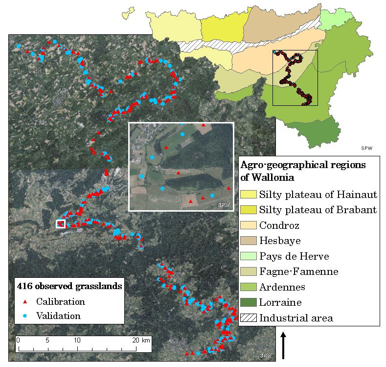
This study was performed on permanent grasslands in Wallonia, the Southern region
of Belgium, covering 16,901 km2 (Figure 1). Permanent grasslands cover 35% of the utilised
agricultural area (UAA) of the Walloon region [33]. Grasslands are defined as permanent
in the regional land parcel identification system (LPIS) [34] when no crop rotation has
occurred for at least 5 years. The number of parcels and the management intensity vary
across the different agro-geographical areas of the region (Figure 1). The delimitation of
these areas is based on agro-ecological conditions and cropping systems. The present
study encompasses a significant diversity of agro-ecological and farming conditions and
includes Condroz, Fagne-Famenne and Ardennes, with respectively about 37%, 71% and
88% of the UAA occupied by grasslands [35]. Other agricultural areas dominated by
grasslands include Pays de Herve and Lorraine, which were not covered in this study
for field campaign feasibility reasons. This study focuses more precisely on grasslands
classified as “E 2.1 Permanent mesotrophic pastures and aftermath grazed meadows”
and “E2.2 Low and medium altitude hay meadows” in the European Nature Information
System (EUNIS). The first class includes permanent pastures and mixed mowing and
grazing management. The second class, which is strictly mown with no grazing activity,
has become scarcer over the past decades [36]. The first mowing date differs depending on
the grassland management. In most common grasslands, exploitation activities (grazing
and/or mowing) start from mid-April. In grasslands of high biological interest, supported
by the EU Common Agricultural Policy, mowing is only allowed after 16 June, for flowering
purposes, and before 31 October.Remote Sens. 2021, 13, 348 4 of 18
Figure 1. Location of the grassland parcels monitored during the windshield survey across 3
main agro-geographical regions of Wallonia (Condroz, Fagne-Famenne and Ardennes). The set of
416 parcels was split in two subsets for calibration and validation of the mowing detection methods.
3. Data
3.1. Field Data
An intensive field campaign was carried out to collect reference data for the develop-
ment, calibration and quantitative performance assessment of mowing detection methods.
Between mid-April and mid-July 2019, 11 visits were undertaken on (or near) Sentinel-1
acquisition dates (Figure 2). The campaign was based on a windshield survey through-
out the study area. During each visit along the same route, all permanent grasslands
were observed from the road and the management status of each parcel was registered
as ‘growing’ when no activity could be observed, ‘recently cut’, ‘being cut’ or ‘grazed’
when livestock was present on the parcel. This survey provided information for 10 time
intervals on a set of 416 permanent grasslands resulting in a total of 4160 observation
intervals. The surveyed grasslands were located in different agro-geographical regions: 76
in Condroz, 190 in Fagne-Famenne and 150 in Ardennes. The field visits were carried out as
much as possible at a 6-day pace, corresponding to the Sentinel-1 A and B combined revisit
cycle, with the highest frequency in May and June, when the first cuts are expected to occur
and the regrowth would be relatively fast. Observations were made with intervals of 6, 12
or 18 days. Overall, 236 mowing events were recorded during the study period. The set
of monitored parcels was split into two independent subsets for calibration (n = 220) and
for validation (n = 196) (Figure 1). The subsets were built by stratified random sampling,
ensuring that three types of grasslands are represented in each. The first type are parcels in
which at least one mowing event was observed but no grazing. They are further referred
to as ‘hay meadows’. In the second type, further referred to as ‘mixed practices’, bothRemote Sens. 2021, 13, 348 5 of 18
mowing and grazing events were observed. In the third type of parcels no mowing events
were registered during the study period, but grazing livestock was observed at least once
in each. They are further referred to as ‘unmown pastures’.
Figure 2. Sentinel-1 A and B (descending) acquisition dates over the study area and corresponding
field observation dates between April and July 2019.
3.2. Sentinel-1 Time Series
Sentinel-1 data was acquired in Single Look Complex (SLC) format and interferometric
wide (IW) swath mode with dual polarisation (vertical transmission with vertical reception
(VV) or horizontal reception (VH)). The processing to Ground Range Detected (GRD)
backscattering coefficient (γ0 ) and interferometric coherence with a 15 m resolution was
performed using the Sentinel-1 Toolbox of ESA’s SNAP (version 6.0). The processing chains
shown in Figure 3 include calibration, georeferencing, deburst, InSAR coherence estimation
(with an averaging window size of azimuth × range: 3 × 10) and terrain correction. Both
chains were run on acquisitions from Sentinel-1 descending pass covering Wallonia during
2019. Only descending pass acquisitions were treated in this study, because coherence
should not be computed between different passes (ascending or descending) since the
look direction varies. Moreover, field visits were carried out with a minimum interval of
6 days, matching just descending pass acquisition dates, for practical and timely reasons.
Coherence was computed between consecutive Sentinel-1 A and B images, in order to
reach a 6-day revisit cycle instead of 12, as suggested by [31].
SAR imagery is characterised by an inherent variance (speckle) caused by constructive
and destructive interference between randomly distributed scatterers inside a pixel [37].
This speckle effect can be observed on apparent homogeneous surfaces, such as herbaceous
covers. In order to spatially smooth the SAR data, the regional LPIS layer [34]—established
on an annual basis by the Walloon Administration for the EU Common Agriculture Policy
and referencing the localisation, the extent and the main crop of agricultural parcels in
Wallonia—was used to average the backscattering and coherence signal per parcel. A 10 m
inner buffer was applied to the parcel polygons before averaging, in order to reduce
border effects.
Figure 3. Schematic overview of the Sentinel-1 processing chain from single look complex (SLC)
interferometric wide (IW) swath mode with dual polarisation (VV, VH) to Ground Range Detected
(GRD) backscattering coefficient (γ0 ) and interferometric coherence with a 15 m resolution. Processing
performed using the Sentinel-1 Toolbox of ESA’s SNAP (version 6.0).
4. Methods
Several mowing detection methods were selected based on previous studies and
time series observation, and compared to each other. The methods are based on change
detection in time series of a backscattering coefficient on the one hand and of interferometric
coherence on the other. All methods were tested using VV and VH signal, as well as a
combination of both polarisations, namely the ratio (VV/VH) in the case of backscattering
and the average (mean(VV,VH)) in the case of coherence.Remote Sens. 2021, 13, 348 6 of 18
4.1. Backscattering Detection Method
This first method, based on γ0 backscattering time series, consists of detecting the
occurrence of a signal increase followed by a signal decrease, with respective threshold
magnitudes, which have been observed after mowing events in several studies [24,25,38].
The change in backscattering after a mowing event could be linked to a stronger contribu-
tion of soil surface scattering, compared to the volume scattering of the vegetation on tall
grass. The method selected here is largely based on the two axioms used by [24], namely
(1) the occurrence of a signal increase followed by a decrease and (2) the magnitude of
those changes above a fixed threshold. For each parcel extracted time series, each value γi
is compared to the previous γi−1 and the next γi+1 . Two conditions then need to be met.
(1) The value γi needs to be larger than the previous value γi−1 and the next value γi+1 :
γi − 1 < γi > γi + 1 (1)
(2) The amplitude of the changes, expressed as per cent increase Dup and decrease Ddown :
γ − γi − 1
Dup = 100 ∗ ( i ) (2)
γi
| γi + 1 − γi |
Ddown = 100 ∗ ( ) (3)
γi
must be higher than the average per cent increase and decrease by a fixed threshold (Kup %
and Kdown %, respectively). The average per cent change describes the signal variation along
the entire time series and is computed for each parcel, to be used in the following equations:
| γi − γi − 1 |
∑iN=0 γi ∗ 100
Dup − ≥ Kup % (4)
N
and
| γi + 1 − γi |
∑iN=0 γi ∗ 100
Ddown − ≥ Kdown % (5)
N
A detection is made when Equations (1), (4) and (5) are true. This method was tested
with different threshold values Kup % and Kdown % (Table 1).
Table 1. Overview of the considered mowing detection methods. The backscattering methods were tested with different
input polarisations, per cent increase thresholds (Kup %) and different ratios between per cent decrease and increase
thresholds (Kdown /Kup ). The coherence jump detection methods were tested with different polarisations, smoothing
approaches, window sizes (d) and absolute thresholds (a.t.,k) or relative threshold (r.t.) parameters (α).
Input Per Cent Increase Threshold Kup % Ratio (Kdown /Kup )
Backscattering (γ):
2 ; 5 ; 10 ; 15 ; 20 ; 25 1/4 ; 1/2 ; 3/4 ; 1
VV, VH, ratio
Input Smoothing Window Size (d) Detection Threshold Parameter
Absolute (a.t) k= {0.5, 0.25, 0.1, 0.075,
Mean shift 7 ; 9 ; 11
Coherence: 0.05, 0.025, 0.01, 0.005, 0.0025} ;
cohVV; cohVH; Relative (r.t.) α= {0.0005, 0.001, 0.005,
Linear regression 3;4;5;6
cohVVVH 0.01, 0.025, 0.05, 0.1, 0.2, 0.4}
p-value = {0.01, 0.02, 0.03, 0.04, 0.05,
Two means 8 ; 10
0.06, 0.07, 0.08, 0.09, 0.1, 0.25, 0.5, 0.75}
4.2. Coherence Jump Detection Methods
The second set of methods is based on the observation of a high jump in coherence
time series right after a mowing event. A mowing event implies a drastic reduction
of above ground biomass. According to observations made in previous studies [30,31],Remote Sens. 2021, 13, 348 7 of 18
such a reduction in biomass causes a sudden increase from relatively low coherence
values to higher ones for a given period of time after the mowing event, before the grass
grows tall again. Since coherence tends to fluctuate between consecutive dates despite the
spatial filtering, temporal smoothing was applied to reveal significant increases. Based on
preliminary observations of coherence time series on various parcels, three jump detection
methods implying different smoothing approaches were considered (Figure 4).
Mean shift: The first method, called mean shift, consists in a sliding averaging
window of a maximum size d with an adjusting symmetry. It allows to smooth the signal
while highlighting significant shifts in the temporal mean such as jumps. When applying
the mean shift sliding window, each raw value Ti is replaced by the average of [Ti−r1 ,Ti+r2 ],
resulting in a smoothed value ms( Ti ). The number of points before (r1 ) and after (r2 )
included in the window are adapted to the local variance of the signal in each window.
They are defined by the following limits (Equation (6)) resulting in a maximum window
size d = 2 ∗ rmax + 1. ( (
r1 = rmax r1 = [0, rmax ]
OR (6)
r2 = [0, rmax ] r2 = rmax
Between those limits, the window symmetry parameters r1 and r2 adjust for each
window to minimize the standard error of the average (σx ):
σ[Ti−r ,Ti+r ]
1 2
σx = √ (7)
r1 + r2 + 1
where σ is the standard deviation of [Ti−r1 ,Ti+r2 ]. Jumps are detected between smoothed
values when the difference ms( Ti ) − ms( Ti−1 ) exceeds a fixed threshold. The method was
tested with absolute thresholds (a.t.) (k) or relative thresholds (r.t.) to the standard error.
In the second case, a Student’s test (t-test) with a given significance level α is performed.
All the tested values for the maximum window size d and the thresholds k and α are
summarised in Table 1.
Linear regression: In the second method, the time series are smoothed by linear re-
gression using an asymmetrical sliding window. Due to the growth of the vegetation prior
to the mowing event, the coherence is expected to gradually decrease and then suddenly
increase after the mowing event. In this method, each raw value Ti is compared to the previ-
ous smoothed value lr ( Ti−1 ) obtained by linear regression of [ Ti−d , ..., Ti−1 , Ti ]. This allows
to consider a potential slope in the coherence profile and detect sudden increases, compared
to the previous signal trend. A detection is made when the difference Ti − lr ( Ti−1 ) exceeds
a given threshold. This method was also tested with different window sizes d, and absolute
(k) and relative (α) thresholds (Table 1).
Two means: The third jump detection method is based on a sliding window of even
size d in which a statistical hypothesis test verifies if there is a significant change in temporal
mean coherence in the middle of the window. This is another way to detect a sudden
increase in a coherence time series. The null hypothesis H0 is the approximation by the
average value of the whole window mean([ T1 : Td ]). The alternative hypothesis H1 is
the approximation by a “step model” consisting of two different averages for the first
half [ T1 : Td/2 ] and second half [ Td/2+1 : Td ] of the window. The Fstat used for the test is
computed via Equation (8):
SSR0 −SSR1
k1 −k0
Fstat = (8)
SSR1
d−k1
where SSR[0,1] and k [0,1] are, respectively, the Sum of Squared Residuals and the number
of parameters of H[0,1] . The probability density function of Fstat is derived from n, k0 and
k1 and a p-value is computed for each date. A p-value under a given threshold implies
a rejection of H0 . In that case, and if the second mean value is higher than the first,
a coherence jump is detected. Table 1 gives an overview of all the coherence jump detection
methods applied using the different inputs, window sizes and detection thresholds.Remote Sens. 2021, 13, 348 8 of 18
Figure 4. Schematic representation of the 3 coherence jump detection methods. A jump occurs
at Ti . (a) The mean shift method with maximum window size d = 2 ∗ rmax + 1 = 9 (r1 = 0
and r2 = rmax = 4), where the difference (red arrow) between the smoothed values is evaluated,
(b) the linear regression method with window size d = 4, where raw value Ti is compared to the
previous smoothed value and (c) the two means method of window size d = 8, comparing the
hypothesis H0 (1 mean) and H1 (2 means).
4.3. Method Calibration, Evaluation and Validation
The calibration step aimed at identifying the best parameters for each backscattering
and coherence jump detection methods, i.e., optimal window sizes and values of the
detection thresholds. It was also used to analyse the robustness of these methods to the
major confounding factors related to the use of Sentinel-1 data.
The calibrated methods were validated on an independent set of grassland parcels
to estimate the potential of Sentinel-1 based mowing detection for identifying different
grassland mowing dynamics.
In order to identify optimal parameters, calibration was performed on a subset of
the calibration data set with parcels presenting ideal size, shape and slope orientation.
Those ideal parcels have an area larger than 1 ha, a width larger than 30 m and the hill
shade has to be above the median of the data set. Hill shade was used as indicator for
slope orientation, as it is based on the orientation of the slope relative to an illumination
source angle and shadows. These three requirements correspond to parcel characteristics
potentially affecting the Sentinel-1 signal. Small parcels are expected to be more challenging
to monitor because of the limited amount of pixels included in the spatial smoothing.
The shape of a parcel could be an issue because narrow parcels might be impaired by
border effects (mixed pixels). Finally, the orientation of the slope relative to the radar beam
direction will have an impact on the signal interaction with the surface.
The calibrated methods were then applied on parcels presenting less ideal character-
istics in order to observe the impact of size, shape and slope orientation on the mowing
detection accuracy. In addition to parcel characteristics, the robustness of the methods to
grazing activities was assessed. Based on the in situ observations, the data set was split
into grazed parcels on which no mowing event was observed, grazed parcels where at least
one mowing event was observed and parcels that were mown, but not grazed during the
period of observation. These are further referred to as ‘unmown pastures’ (n = 105), ‘mixed
practices’ (n = 36) and ‘hay meadows’ (n = 79), respectively.
Quality metrics for calibration and robustness analysis were computed using the
time intervals between field visits on each parcel as the unit. There are 10 intervals for
each of the 220 parcels selected for calibration, resulting in a total of 2200 observations.
Each time interval of each parcel can then be labelled with: the occurrence of mowing
event (1) or the absence of mowing event (0), according to field observation and Sentinel-1
mowing detection. Based on the cumulative count of intervals of all parcels, confusion
matrices were built between observed and detected mowing events. Since mowing events
are relatively rare, there is a strong imbalance between (1) and (0). Therefore, in addition to
the broadly used overall accuracy (OA), the Matthews Correlation Coefficient (MCC) was
used for calibration and evaluation, along with the sensitivity and precision of mowing
detection. The MCC was first introduced by Matthews [39] and the metric is particularly
suited to measure the quality of an unbalanced binary classification [40]. The MCC valuesRemote Sens. 2021, 13, 348 9 of 18
range from −1 to 1, 0 being the equivalent of a random classification. The sensitivity is a
measure of the detection rate and the precision measures the fraction of detections that are
true positives. The MCC metric, the sensitivity and the precision are computed, based on
the true (T)/false (F) positives (P) and negatives (N), using Equations (9)–(11).
TP ∗ TN − FP ∗ FN
MCC = p (9)
( TP + FP)( TP + FN )( TN + FP)( TN + FN )
TP
Sensitivity = (10)
TP + FN
TP
Precision = (11)
TP + FP
The best performing and most robust method was then applied to the independent
validation data set of 196 parcels. In this case, the performances were evaluated per
parcel, instead of per time interval. The aim is to assess the potential of Sentinel-1 based
mowing detection methods for identifying different mowing dynamics of grasslands.
The assessment was performed for four types of grassland management observed during
the field campaign: (i) unmown pastures, (ii) parcels with 1 spring mowing (before 20 June),
(iii) with 1 summer mowing and (iv) with 2 mowing events during the study period.
For type (i), the potential for identification was assessed by counting the parcels with no
detection (identified correctly) and the parcels with at least one false detection. For types
(ii) and (iii), the parcels where the mowing event (spring or summer) was detected with no
false detection were counted as correctly identified. A further distinction was then made
between parcels with false detection, omission or both. Finally, for type (iv), the number of
cases in which the two events are detected with no false detection (identified correctly),
in which only the first or the second event is detected, in which both are omitted and in
which only false detections are made, were counted.
5. Results
5.1. Method Calibration
All methods were run on the ideal calibration parcels with a range of different detec-
tion parameters (Table 1). In total, 12 configurations were considered for methods based
on backscattering. For coherence jump detection, 48 different configurations of polarisa-
tion, smoothing approach, window size and threshold type were considered. The first
observation is that the detection method based on backscattering performed very poorly
compared to the coherence jump detection methods. The maximum MCC obtained with
backscattering is 0.25, using γ0 VV time series, while the highest MCC values obtained
with the different coherence jump detection methods range from 0.26 to 0.49. The focus
was therefore set on coherence jump detection methods for further analysis.
The different smoothing methods, window sizes and threshold types are compared
based on the OA, the sensitivity, the precision and the MCC along the different detection
threshold values (Figure 5). The OA (unbroken blue line) reaches high values ranging from
92% to 96% for all methods. It drops significantly with low absolute detection thresholds
(a.t.), for example, to 45% for k = 0.0025 with the cohVV linear regression method (d =
6), because of the numerous false detections made with such a low detection threshold
(Figure 5d).
As expected, when the detection threshold increases (1 −α, 1 − p-value and k), the pre-
cision increases as less false detections occur, but the sensitivity declines as more mowing
events are omitted. No significant difference was observed in the shapes of the sensitiv-
ity and precision curves, between the different input polarisations (cohVV, coh VH and
cohVVVH) or window sizes. On the other hand, the shape of the curves vary from one
smoothing method to another as shown in Figure 5. Both with absolute and relative thresh-
olds, the threshold value at which precision and sensitivity reach a balance and the curves
cross, is higher for the linear regression method than for the mean shift. For the mean shiftRemote Sens. 2021, 13, 348 10 of 18
method (Figure 5a,b), when α tends toward 0 or k increases, the sensitivity drops relatively
low as the detections become more precise. Meanwhile for the linear regression method
(Figure 5c,d), the sensitivity remains high with more precise detection thresholds. For the
two means smoothing method, the sensitivity also drops relatively fast while the precision
does not increase significantly.
The MCC metric (dashed blue line), peaks above 0.4 for all methods except for the
two means method (Figure 5e). The two means method was therefore also discarded for
further analysis. The MCC peak was used here to select the best performing methods and
detection thresholds. However, even at these optimal thresholds, either the precision or the
sensitivity are lower than 50% for all methods.
Figure 5. Overall Accuracy (OA), Matthews Correlation Coefficient (MCC), precision and sensitivity
of several mowing detection methods based on VV coherence, with varying detection threshold
parameters. The graphs show the performances of the mean shift and linear regression methods with
relative threshold (r.t.) and absolute threshold (a.t.) and of the two means method, with the best
window size (d) for each.
For further analysis, the two methods delivering the highest MCC value were selected
for VV coherence (cohVV), VH coherence (cohVH) and the average of VV and VH coherence
(cohVVVH). The six selected methods are (i) cohVH mean shift (d = 9) with relative
threshold (α = 0.001), (ii) cohVH linear regression (d = 5) with r.t. (α = 0.0005), (iii) cohVV
mean shift (d = 11) with a.t. (k = 0.025), (iv) cohVV linear regression (d = 6) with r.t.
(α = 0.005), (v) cohVVVH linear regression (d = 5) with a.t. (k = 0.1) and (vi) cohVVVH
linear regression (d = 6) with r.t. (α = 0.005). The MCC values obtained for these methods
range from 0.44 for (ii) to 0.49 for (iv). These calibrated methods are listed in Table 2.
5.2. Robustness to Confounding Factors
In order to analyse the robustness of the mowing detection methods, the impact
of parcel characteristics on the sensitivity (Sen) and precision (Pre) of the detection was
analysed. The results obtained for ideal, small and narrow parcels, for parcels with lower
hill shade values, for all non ideal parcels and for all parcels are listed in Table 2.
On the ideal parcels, the calibration based on MCC metrics resulted in a balance
between omissions and false detections, depending on the methods. The cohVH mean shift
method shows the least balance, with the highest precision (78%) and the lowest sensitivity
(27%). The most balanced calibrated method is cohVVVH linear regression with absolute
threshold, with a precision and sensitivity of 42% and 54%, respectively. Both methods with
VH coherence were calibrated with a higher precision, while the methods with cohVV and
cohVVVH resulted in higher sensitivities at the optimal threshold. The highest sensitivityRemote Sens. 2021, 13, 348 11 of 18
(69%) on ideal parcels was obtained with both cohVV methods and the cohVH linear
regression method with relative threshold.
Among the parcel characteristics the most significant impact is observed for narrow
parcels, as both precision and sensitivity are significantly lower for all methods. The largest
impact of parcel shape is observed with the cohVH mean shift method, which was also
the least balanced. The precision and sensitivity of this method respectively dropped to
13% and 8% on the narrow parcels. The individual effects of size and slope orientation on
the accuracy of mowing detection are less significant or consistent through the different
methods. Some positive impacts are even observed on the precision.
In order to observe the combined impact of the three parcel characteristics on the sensitiv-
ity and precision of mowing detection, ideal and non ideal parcels are compared (Figure 6a).
For all methods the sensitivity is lower on non ideal parcels. The effect on the precision is,
however, more variable. The most robust methods are cohVH linear regression and both
cohVVVH linear regression methods, for which the sensitivity and precision vary by less than
10% between ideal and non ideal parcels. For cohVV linear regression, the precision is not
impacted by the parcel characteristics, but the sensitivity drops by 20%. As before, the largest
impacts are observed on cohVH mean shift, where the precision drops by 31%.
Then the impact of grazing activities on the detection accuracy was assessed, thanks
to the observations made during the field campaign (Figure 6b). As expected the sensitivity
does not vary when unmown pastures are removed from the data set. The precision is
however significantly higher for all methods, namely 64% for cohVVVH linear regression
with a.t., 72% for cohVV linear regression and 86% for cohVH linear regression, while these
methods have precisions of 43%, 42% and 57%, respectively, when considering all types
of grasslands. This means that a large part of the false detections was due to unmown
pastures. When removing the mixed practices and considering only the hay meadows,
the precision and sensitivity barely change and no consistent impact is observed through
the different methods.
The most important increase of precision (+30%) after discarding unmown pastures
was observed for the cohVV linear regression method (d = 6) with r.t. (α = 0.005), which
has a reasonable sensitivity of 54% on all parcels and reached a 69% detection rate on
parcels with ideal characteristics. It was therefore selected as the overall best performing
method and used for further parcel-based validation.
Figure 6. Robustness of calibrated Sentinel-1 coherence mowing detection methods to parcel char-
acteristics (size, slope orientation and shape) and grazing practices. Graph (a) shows the changes
in precision and sensitivity between detections on large, broad and well oriented parcels (ideal)
and on parcels with less ideal characteristics (non ideal). Graph (b) shows the changes in precision
and sensitivity when removing unmown pastures (p) and then mixed practices (x), considering hay
meadows (m) alone.Remote Sens. 2021, 13, 348 12 of 18
Table 2. Impact of the size, topography and shape of the parcels on the accuracy of calibrated mowing
detection methods, based on VH coherence (cohVH), VV coherence (cohVV) and the average of VV
and VH coherence (cohVVVH) with absolute (a.t.) and relative (r.t.) threshold and window sizes d.
The threshold parameters α and k were optimised based on the Matthews Correlation Coefficient
(MCC), to obtain a balance between precision (Pre) and sensitivity (Sen).
Ideal Small Slope Dir Narrow Non Ideal All
n 590 430 770 330 1470 2200
cohVH mean shift (d = 9) r.t. (α = 0.001)
Pre 78 50 53 13 47 57
Sen 27 8 20 8 18 22
cohVH linear reg. (d = 5) r.t. (α = 0.0005)
Pre 60 63 59 33 51 54
Sen 35 21 31 15 23 25
cohVV mean shift (d = 11) a.t. (k = 0.025)
Pre 48 35 44 25 40 42
Sen 69 63 59 31 47 53
cohVV linear reg. (d = 6) r.t. (α = 0.005)
Pre 38 32 44 32 39 39
Sen 69 42 57 46 49 54
cohVVVH linear reg. (d = 5) a.t. (k = 0.1)
Pre 42 32 44 26 38 38
Sen 54 63 45 46 43 45
cohVVVH linear reg. (d = 6) r.t. (α = 0.005)
Pre 34 46 49 30 44 41
Sen 69 50 67 46 59 61
5.3. Parcel-Based Validation
The calibrated cohVV linear regression (d = 6) method with r.t. (α = 0.005) was
applied on the independent validation data set of 196 parcels, for grassland management
classification (Figure 7). The aim is to assess the performances for identifying different
mowing dynamics of grasslands, based on Sentinel-1 mowing detection.
From the 100 unmown parcels, which were all grazed during the study period, 54%
were correctly identified as unmown (first bar of Figure 7), meaning false detections
were made in almost half of the unmown pastures. This confirms the results of the
robustness analysis, identifying grazing as a major confounding factor to mowing detection
with Sentinel-1.
The second bar of Figure 7 shows the performances on the 26 parcels with one spring
mowing. Here too, 54% were correctly identified. In the remaining spring mowing parcels
the mowing event was omitted and in four parcels (15%) a false detection was made in
addition to the omission. Much better results were obtained with summer mowings
(third bar of Figure 7), as 71% of the 51 parcels with one summer mowing were correctly
identified. A second false detection was made in eight parcels (16%), the summer mowing
event was omitted in seven parcels (14%), in two of which a false detection was made in
the spring.
Finally, from the 19 parcels with two mowing events (fourth bar of Figure 7), only
six (32%) were entirely correct. Here as well, most of the summer events were detected
(12 parcels or 64%), while many spring mowings were omitted (nine parcels or 48%).
Both mowing events were omitted in only four parcels, one of which also counted as a
false detection.Remote Sens. 2021, 13, 348 13 of 18
Considering the whole validation data set, 56% of all parcels and 59% of the mown
parcels were identified correctly in terms of mowing dynamics, based on Sentinel-1 co-
herence mowing detection. Most errors consist of false detections in grazed parcels and
omitted spring mowing events.
Figure 7. Per parcel evaluation of Sentinel-1 VV coherence mowing detection (smoothed by linear
regression, with window size d = 6 and relative threshold (α = 0.005)) potential to identify different
mowing dynamics. For each type of dynamic, the fraction of correctly estimated parcels are given,
along with the types of errors that occur (false detections, omissions or both).
6. Discussion
The results of this study corroborate the potential for detecting mowing events using
InSAR coherence, as already suggested by a study on a limited number of grassland
parcels [31]. Overall, it was shown that mowing events can be detected by identifying
jumps in coherence time series. Based on a large and diverse reference data set, numerous
methods could be developed, calibrated and thoroughly analysed on different types of
grassland. Once calibrated, most methods showed similar performances and robustness.
Nevertheless, the mowing detections based on VV coherence smoothed by linear regression
with a window d = 6 and a relative threshold (α = 0.005) were slightly more precise and
accurate, especially on hay meadows.
6.1. Mowing Detection Methods
The methods based on the hypothesis of occurrence of an increase and subsequent
decrease in backscattering after a mowing event performed poorly during the calibration
phase. The authors of [24] accurately detected all mowing events in two semi-natural
meadows, using TerraSAR-X σ0 images, while this study used Sentinel-1 C-band γ0 . Their
mowing detection method should therefore be further tested with X-band SAR data on a
larger and richer data set.
On the other hand, it was shown that mowing events can be detected by identifying
jumps in smoothed coherence time series. The ’two means’ smoothing method could
be discarded based on lower MCC values, but performances varied little between the
different input polarisations, window sizes and detection threshold types for the mean
shift and linear regression methods (Table 1). In ideal cases, the mowing event causes
such an ample coherence increase that it is easily detected, whatever the method. To the
contrary, regardless of the method and parameters, some mowing events cannot be detected
at all and coherence jumps can be caused by signal noise or other surface changes. As
an illustration, eight coherence time series extracted on different types of parcels, along
with the mowing events observed on the field are shown in Figure A1 (Appendix A).
Hence, most of the errors are independent of the detection method but inherent to the
signal and its interactions with other factors. In order to understand the causes of theseRemote Sens. 2021, 13, 348 14 of 18
limitations, a robustness analysis was carried out to identify the confounding factors to
mowing detection with Sentinel-1 coherence.
6.2. Limitations
The sensitivity and precision metrics in Table 2 and Figure 6 show that the size, shape
and slope orientation of the parcels can hinder the detection of mowing events for most
methods. Fewer mowing events are detected in small or narrow parcels or parcels with
a less ideal slope orientation and with some methods, more false detections are made in
these less ideal parcels. The differences in accuracy are, however, minor and not always
consistent throughout the methods.
From the confounding factors tested in this study, grazing is clearly the most important
one. Many false detections were made in parcels that were not mown, but grazed during
the study period. During validation, false detections were made in almost half of the
unmown pastures, confirming that grazing is a major confounding factor to mowing
detection. As coherence increases with decreasing grass height and biomass [30], a grazing
event with a large stock density could in fact result in a coherence jump, similar to a
mowing event.
In hay meadows and mixed practice parcels, the coherence jump detection method
developed in this study allowed to detect most summer mowings, both when they were
first or second mowing events, while about half of the spring mowings were omitted
(Figure 7). This could be explained by a slower regrowth of the grass after summer cuts,
causing the coherence to remain high for a longer period and making the detection easier.
The confounding factors assessed in this study explain some of the false detections
and missed mowing events. However, in a number of cases the cause of errors remains
unclear. Other factors could hinder the detection of mowing events by impacting the radar
signal, such as the presence of trees and shrubs or the soil and plant water content. The
impact of water content on radar signal has already been shown previously [23]. It was
also shown to be a potential confounding factor to mowing detection [25,31]. In terms of
agricultural practices, swaths of grass left on the parcel to dry could also be a confounding
factor that alters the signal response after a mowing event.
The mowing detection method developed in this study is object-based and relies on
the availability of grassland parcel boundaries for spatial smoothing. The regional LPIS
provided this information for this study area. The LPIS parcels are, however, based on
farmer declarations, hence partially mown parcels could be a cause for errors. Alterna-
tively, parcel boundaries could be retrieved through automatic delineation based on a
convolutional neural network (CNN) [41].
6.3. Reference Data and Quality Metrics
The major limiting factor in the development and evaluation of mowing detection
methods is the availability of precise and complete field data [32]. The large field campaign
carried out in the frame of this study provided information on the land use status of
more than 400 agricultural grassland parcels across different agro-geographical regions of
Wallonia, on Sentinel-1 acquisition dates. Thanks to this rich data set, it was possible to
statistically evaluate the mowing detection potential of Sentinel-1 in agricultural grasslands.
The choice of adequate quality metrics that properly show the performances of a
detection method with respect to the context and overarching goal, is another critical point.
In the case of the detection of a rare event, the classes of occurrence and absence of the
event are unbalanced. Because of that disproportion, the broadly used overall accuracy
(OA) is mainly influenced by the numerous absences and is not representative of the
detection accuracy. Indeed, the OA reached values above 90% for all methods during
calibration, while the detection sensitivity and precision were relatively low (Figure 5).
The sensitivity and the precision focus on the true positives, false positives and false
negatives and clearly represent the performances of a detection method from the point of
view of the events occurrence. Increasing the detection threshold enhances the precision,Remote Sens. 2021, 13, 348 15 of 18
but reduces the sensitivity, as more events are omitted. When calibrating the mowing
detection methods, a compromise needs to be made between maximising the detection
rate and minimising the false detections. In this study, the MCC metric was used to
calibrate the methods and select the optimal detection thresholds as it is well adapted for
unbalanced binary classifications [40]. Depending on the methods, this resulted in a higher
precision or a higher sensitivity and more or less balance between both metrics. In practice,
the detection threshold needs to be set according to the context and the motivation for
mowing events detection.
6.4. Potential and Prospects
The Sentinel-1 coherence mowing detection method developed in this study allows
to detect most summer mowings in hay meadows. However, considering the diversity of
grassland types and management dynamics, the mowing detection lacks precision and
some mowing events cannot be detected based only on Sentinel-1 coherence.
In order to enhance the precision, it would be a great asset to differentiate grazed
parcels from hay meadows beforehand, as most false detections were made in pastures.
Previous studies have been discriminating grazed grasslands from hay meadows, based,
for example, on backscattering coefficients [25] or vegetation indices derived from optical
imagery [14].
In the prospect of grassland use intensity assessment and habitat monitoring, it is
critical to be able to detect early spring mowing events with more certainty, in order
to differentiate more intensively managed grasslands from extensive grasslands with a
higher ecological value. The performances could probably be improved by combining
the Sentinel-1 coherence mowing detection, calibrated to obtain a high precision, with an
optical method based on decreases in NDVI, such as [15] or [17].
7. Conclusions
The main goal of this study was to assess the full potential of Sentinel-1 for detecting
mowing events, by estimating the accuracy of mowing detection, identifying the main
limitations and confounding factors and finally evaluate the potential for predicting differ-
ent types of grassland mowing dynamics. Using timely field data on the state and use of
416 grassland parcels, four Sentinel-1-based mowing detection methods were evaluated
with various parameter configurations on diverse grasslands. The methods were based on
two main observations of SAR signal response to a mowing event, namely the occurrence
of a backscattering signal rise and decrease and of an interferometric coherence jump.
While the methods based on backscattering showed very low performances, the coherence
jump detection methods allowed to accurately detect a majority of mowing events in hay
meadows. However, due to the omission of a significant amount of spring mowings and
many false detections in pastures, only 56% of grasslands in a fully independent data set
were identified correctly in terms of mowing dynamics. The size, shape topography and
agricultural practices explain some of the errors, but a part remains uncertain and must
be due to other signal interactions. The results of this study confirm that it is feasible to
detect mowing events based on coherence jumps. The performances could probably be
further enhanced by discriminating pastures beforehand and combining Sentinel-1 and
Sentinel-2 data. However, a compromise will always have to be made between sensitivity
and precision and the detection threshold needs to be set accordingly, depending on the
context and the purpose of mowing detection.
Grassland mowing detection represents a great asset for estimating grassland use
intensity in the context of large scale habitat quality monitoring. Methods to detect mowing
events should therefore be further studied and developed using large, diverse and precise
field data sets.
Author Contributions: Formal analysis, M.D.V.; investigation, M.D.V.; methodology, M.D.V.; super-
vision, J.R. and P.D.; validation, J.R. and P.D.; writing—original draft preparation, M.D.V.; writing—Remote Sens. 2021, 13, 348 16 of 18
review and editing, J.R. and P.D. All authors have read and agreed to the published version of the
manuscript.
Funding: This research is part of the LifeWatch FWB project in the context of the ESFRI and supported
by Fédération Wallonie Bruxelles.
Institutional Review Board Statement: Not applicable.
Informed Consent Statement: Not applicable.
Data Availability Statement: Data sharing not applicable. No new data were created or analyzed in
this study. Data sharing is not applicable to this article.
Acknowledgments: We acknowledge the Walloon Administration for the land parcel identification
system (LPIS) layer used as a spatial filter to extract time series per parcel.
Conflicts of Interest: The authors declare no conflict of interest.
Abbreviations
The following abbreviations are used in this manuscript:
EUNIS European nature information system
GRD Ground range detected
InSAR Interferometric SAR
LPIS Land parcel identification system
MCC Matthews correlation coefficient
NDVI Normalised difference vegetation index
OA Overall accuracy
SAR Synthetic aperture radar
SLC Single look complex
UAA Utilised agricultural area
Appendix A
Figure A1. Sentinel-1 VV coherence time series extracted from a selection of 8 grassland parcels
(2 mixed practices, 3 hay meadows and 3 unmown pastures). The green areas represent time intervals
in which a mowing event occurred according to field observations. The green line represents a
mowing event observed on the day of a field visit.Remote Sens. 2021, 13, 348 17 of 18
References
1. Hansen, M.C.; Defries, R.S.; Townshend, J.R.G.; Sohlberg, R. Global land cover classification at 1 km spatial resolution using a
classification tree approach. Int. J. Remote Sens. 2000, 21, 1331–1364. [CrossRef]
2. Loveland, T.R.; Reed, B.C.; Brown, J.F.; Ohlen, D.O.; Zhu, Z.; Yang, L.; Merchant, J.W. Development of a global land cover
characteristics database and IGBP DISCover from 1 km AVHRR data. Int. J. Remote Sens. 2000, 21, 1303–1330. [CrossRef]
3. Arino, O.; Ramos Perez, J.; Kalogirou, V..; Bontemps, S.; Defourny, P.; Van Bogaert, E. Global Land Cover Map for 2009 (GlobCover
2009); © European Space Agency (ESA) and Université catholique de Louvain (UCL), PANGAEA: Louvain-la-Neuve, Belgium,
2012. [CrossRef]
4. Tsendbazar, N.; Herold, M.; Mayaux, P.; Achard, F.; Kirches, G.; Brockmann, C.; Boettcher, M.; Lamarche, C.; Bontemps, S.;
Defourny, P. CCI Land Cover Product Validation and Inter-comparison Report; Technical Report; UCL-Geomatics: Louvain-la-Neuve,
Belgium, 2014.
5. Allan, E.; Bossdorf, O.; Dormann, C.F.; Prati, D.; Gossner, M.M.; Tscharntke, T.; Blüthgen, N.; Bellach, M.; Birkhofer, K.; Boch, S.;
et al. Interannual variation in land-use intensity enhances grassland multidiversity. Proc. Natl. Acad. Sci. USA 2014, 111, 308–313.
[CrossRef] [PubMed]
6. Kleijn, D.; Kohler, F.; Báldi, A.; Batáry, P.; Concepción, E.D.; Clough, Y.; Díaz, M.; Gabriel, D.; Holzschuh, A.; Knop, E.; et al.
On the relationship between farmland biodiversity and land-use intensity in Europe. Proc. R. Soc. B Biol. Sci. 2009, 276, 903–909.
[CrossRef] [PubMed]
7. Uematsu, Y.; Koga, T.; Mitsuhashi, H.; Ushimaru, A. Abandonment and intensified use of agricultural land decrease habitats of
rare herbs in semi-natural grasslands. Agric. Ecosyst. Environ. 2010, 135, 304–309. [CrossRef]
8. Zlinszky, A.; Schroiff, A.; Kania, A.; Deák, B.; Mücke, W.; Vári, A.; Székely, B.; Pfeifer, N. Categorizing Grassland Vegetation
with Full-Waveform Airborne Laser Scanning: A Feasibility Study for Detecting Natura 2000 Habitat Types. Remote Sens. 2014,
6, 8056–8087. [CrossRef]
9. Horn, D.J.; Koford, R.R. Relation of Grassland Bird Abundance to Mowing of Conservation Reserve Program Fields in North
Dakota. Wildl. Soc. Bull. 2000, 28, 653–659.
10. Ali, I.; Cawkwell, F.; Dwyer, E.; Barrett, B.; Green, S. Satellite remote sensing of grasslands: From observation to management.
J. Plant Ecol. 2016, 9, 649–671. [CrossRef]
11. Asam, S.; Klein, D.; Dech, S. Estimation of grassland use intensities based on high spatial resolution LAI time series. Int. Arch.
Photogramm. Remote. Sens. Spat. Inf. Sci. 2015, XL-7/W3, 285–291. [CrossRef]
12. Dusseux, P.; Vertès, F.; Corpetti, T.; Corgne, S.; Hubert-Moy, L. Agricultural practices in grasslands detected by spatial remote
sensing. Environ. Monit. Assess. 2014, 186, 8249–8265. [CrossRef]
13. Franke, J.; Keuck, V.; Siegert, F. Assessment of grassland use intensity by remote sensing to support conservation schemes.
J. Nat. Conserv. 2012, 20, 125–134. [CrossRef]
14. Gómez Giménez, M.; de Jong, R.; Della Peruta, R.; Keller, A.; Schaepman, M.E. Determination of grassland use intensity based on
multi-temporal remote sensing data and ecological indicators. Remote Sens. Environ. 2017, 198, 126–139. [CrossRef]
15. Estel, S.; Mader, S.; Levers, C.; Verburg, P.H.; Baumann, M.; Kuemmerle, T. Combining satellite data and agricultural statistics to
map grassland management intensity in Europe. Environ. Res. Lett. 2018, 13, 074020. [CrossRef]
16. Zheng, J.; Li, F.; Du, X. Using Red Edge Position Shift to Monitor Grassland Grazing Intensity in Inner Mongolia. J. Indian Soc.
Remote Sens. 2018, 46, 81–88. [CrossRef]
17. Kolecka, N.; Ginzler, C.; Pazur, R.; Price, B.; Verburg, P.H. Regional Scale Mapping of Grassland Mowing Frequency with
Sentinel-2 Time Series. Remote Sens. 2018, 10, 1221. [CrossRef]
18. Griffiths, P.; Nendel, C.; Pickert, J.; Hostert, P. Towards national-scale characterization of grassland use intensity from integrated
Sentinel-2 and Landsat time series. Remote Sens. Environ. 2020, 238, 111124. [CrossRef]
19. Sano, E.E.; Ferreira, L.G.; Asner, G.P.; Steinke, E.T. Spatial and temporal probabilities of obtaining cloud-free Landsat images over
the Brazilian tropical savanna. Int. J. Remote Sens. 2007, 28, 2739–2752. [CrossRef]
20. Howison, R.A.; Piersma, T.; Kentie, R.; Hooijmeijer, J.C.E.W.; Olff, H. Quantifying landscape-level land-use intensity patterns
through radar-based remote sensing. J. Appl. Ecol. 2018, 55, 1276–1287. [CrossRef]
21. Jacob, A.W.; Vicente-Guijalba, F.; Lopez-Martinez, C.; Lopez-Sanchez, J.M.; Litzinger, M.; Kristen, H.; Mestre-Quereda, A.;
Ziółkowski, D.; Lavalle, M.; Notarnicola, C.; et al. Sentinel-1 InSAR Coherence for Land Cover Mapping: A Comparison of
Multiple Feature-Based Classifiers. IEEE J. Sel. Top. Appl. Earth Obs. Remote Sens. 2020, 13, 535–552. [CrossRef]
22. Shang, J.; Liu, J.; Poncos, V.; Geng, X.; Qian, B.; Chen, Q.; Dong, T.; Macdonald, D.; Martin, T.; Kovacs, J.; et al. Detection of
Crop Seeding and Harvest through Analysis of Time-Series Sentinel-1 Interferometric SAR Data. Remote Sens. 2020, 12, 1551.
[CrossRef]
23. Tampuu, T.; Praks, J.; Uiboupin, R.; Kull, A. Long Term Interferometric Temporal Coherence and DInSAR Phase in Northern
Peatlands. Remote Sens. 2020, 12, 1566. [CrossRef]
24. Schuster, C.; Ali, I.; Lohmann, P.; Frick, A.; Förster, M.; Kleinschmit, B. Towards Detecting Swath Events in TerraSAR-X Time Series
to Establish NATURA 2000 Grassland Habitat Swath Management as Monitoring Parameter. Remote Sens. 2011, 3, 1308–1322.
[CrossRef]
25. Curnel, Y. Satellite Remote Sensing Priorities for Better Assimilation in Crop Growth Models: Winter Wheat LAI and Grassland
Mowing Dates Case Studies. Ph.D. Thesis, UCL-Université Catholique de Louvain, Ottignies-Louvain-la-Neuve, Belgium, 2015.You can also read