A method for computing the three-dimensional radial distribution function of cloud particles from holographic images - Atmos. Meas. Tech
←
→
Page content transcription
If your browser does not render page correctly, please read the page content below
Atmos. Meas. Tech., 11, 4261–4272, 2018
https://doi.org/10.5194/amt-11-4261-2018
© Author(s) 2018. This work is distributed under
the Creative Commons Attribution 4.0 License.

A method for computing the three-dimensional radial distribution
function of cloud particles from holographic images
Michael L. Larsen1,2 and Raymond A. Shaw2
1 Department   of Physics and Astronomy, College of Charleston, Charleston, SC, USA
2 Department   of Physics, Michigan Technological University, Houghton, MI, USA

Correspondence: Michael L. Larsen (larsenML@cofc.edu)

Received: 22 February 2018 – Discussion started: 18 April 2018
Revised: 21 June 2018 – Accepted: 2 July 2018 – Published: 19 July 2018

Abstract. Reliable measurements of the three-dimensional          Shaw, 2003; Marshak et al., 2005; Larsen, 2006; Lehmann
radial distribution function for cloud droplets are desired to    et al., 2007; Salazar et al., 2008; Saw et al., 2008; Small and
help characterize microphysical processes that depend on          Chuang, 2008; Baker and Lawson, 2010; Siebert et al., 2010;
local drop environment. Existing numerical techniques to          Bateson and Aliseda, 2012; Larsen, 2012; Saw et al., 2012b;
estimate this three-dimensional radial distribution function      Beals et al., 2015; Siebert et al., 2015; O’Shea et al., 2016).
are not well suited to in situ or laboratory data gathered           Most of the in situ studies cited above have utilized
from a finite experimental domain. This paper introduces          airplane-mounted cloud probes that report cloud particle po-
and tests a new method designed to reliably estimate the          sitions in a long, thin, pencil-beam-like volume. For exam-
three-dimensional radial distribution function in contexts in     ple, the sample volume of the forward scattering spectrom-
which (i) physical considerations prohibit the use of periodic    eter probe has a cross section of about 0.13 mm2 (Chaumat
boundary conditions and (ii) particle positions are measured      and Brenguier, 2001). These very thin sample volumes have
inside a convex volume that may have a large aspect ratio.        required the majority of the above investigators to treat cloud
The method is then utilized to measure the three-dimensional      particle detections as one-dimensional transects through a
radial distribution function from laboratory data taken in a      three-dimensional medium and appeal to isotropy and spatial
cloud chamber from the Holographic Detector for Clouds            homogeneity to infer three-dimensional statistical properties
(HOLODEC).                                                        (see, e.g., Holtzer and Collins, 2002). Unfortunately, recent
                                                                  work (Larsen et al., 2014) reveals that – even under isotropic
                                                                  and homogeneous conditions – sampling requirements re-
                                                                  quire far more data than initially suspected to reliably recre-
1   Introduction                                                  ate three-dimensional statistics from one-dimensional tran-
                                                                  sects through a cloud.
Cloud droplet clustering is relevant to physical processes           The most direct and assumption-free way to detect cloud
like condensational growth (e.g., Srivastava, 1989; Kostin-       particle clustering is with an instrument that is capable of
ski, 2009), growth by collision–coalescence (e.g., Xue et al.,    recording precise particle locations in all three spatial di-
2008; Onishi et al., 2015), and radiative transfer through        mensions. This can be carried out with a holographic image
clouds (e.g., Kostinski, 2001; Frankel et al., 2017). Conse-      of a cloud volume. Some previous holographic studies that
quently, the magnitude of cloud droplet clustering in situ        explicitly examined three-dimensional cloud particle spatial
and in the laboratory has been a subject of intense interest      distributions have been published (see, e.g., Conway et al.,
for the last 25 years (see, e.g., Baker, 1992; Baumgardner        1982; Kozikowsa et al., 1984; Brown, 1989; Borrmann et al.,
et al., 1993; Brenguier, 1993; Borrmann et al., 1993; Shaw        1993; Uhlig et al., 1998). These pioneering studies were of-
et al., 1998; Uhlig et al., 1998; Davis et al., 1999; Kostinski   ten based on ground-based measurements, included just a
and Jameson, 2000; Chaumat and Brenguier, 2001; Kostinski         few holographic images, and resulted in somewhat conflict-
and Shaw, 2001; Pinsky and Khain, 2001; Shaw et al., 2002;

Published by Copernicus Publications on behalf of the European Geosciences Union.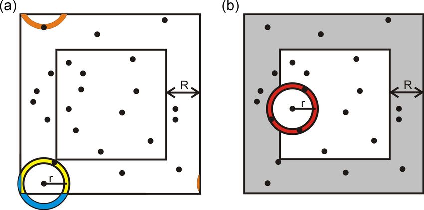
4262          M. L. Larsen and R. A. Shaw: A method for computing the three-dimensional radial distribution function

ing findings. In most cases, the investigators in the above         one-half the smallest length scale defining the measurement
studies argued that holographic imaging looks like a solid          volume L. The new method developed in this paper removes
approach to quantify cloud droplet clustering, but the exces-       both of these limitations.
sive labor required to reconstruct the particle positions from a       The remainder of this paper (i) reintroduces the radial dis-
holographic image made the use of holographic instruments           tribution function, (ii) presents the methods typically used to
impractical for a large-scale study at the time.                    estimate the radial distribution function in different experi-
   Fortunately, both computational and measurement hard-            mental and numerical contexts, (iii) outlines the challenges in
ware capabilities, as well as analysis methods, have improved       utilizing these existing methods for experimental data from
immensely over the last decade, finally bringing holography         modern digital holographic images, (iv) presents and tests
to a fully digital state that allows for data collection and pro-   a new numerical method to calculate the radial distribution
cessing over entire field projects (e.g., Fugal and Shaw, 2009;     function under realistic experimental conditions, and (v) ap-
Beals et al., 2015; O’Shea et al., 2016; Glienke et al., 2017;      plies this method to real data taken by a digital holographic
Schlenczek et al., 2017). For example, the ability to analyze       instrument in a cloud chamber.
three-dimensional clustering in digital holograms has already
been used to identify and eliminate particle shattering effects
(e.g Fugal and Shaw, 2009; Jackson et al., 2014; O’Shea             2   Introduction to the radial distribution function
et al., 2016) or to identify regions of strong entrainment and
inhomogeneous mixing (Beals et al., 2015). These new holo-          The radial distribution function is one of the most widely
graphic instruments should also allow for direct characteri-        used approaches for characterizing particle clustering in tur-
zation of cloud droplet clustering in three dimensions while        bulent flows (Monchaux et al., 2012), and is also currently
obtaining sufficient data to yield unambiguous results.             widely used in a variety of other fields including stochastic
   There are many different mathematical tools utilized to          geometry (e.g., Stoyan et al., 1995), astrophysics (e.g., Mar-
characterize the droplet clustering among cloud droplets,           tinez and Saar, 2001), granular media (e.g., Lee and Seong,
each with their own strengths and weaknesses (see, e.g.,            2016), crystallography (e.g., Cherkas and Cherkas, 2016),
Baker, 1992; Kostinski and Jameson, 2000; Shaw et al.,              and plasma physics (e.g., Erimbetova et al., 2013). The ideas
2002; Shaw, 2003; Marshak et al., 2005; Baker and Law-              behind its use go back at least a century (e.g., Ornstein and
son, 2010; Larsen, 2012; Monchaux et al., 2012). Although           Zernike, 1914), and its wide use permits a large number of
arguments can be made for any number of these tools, this           different conceptual and notational conventions.
study focuses on the radial distribution function (rdf or g(r))        Here, we draw on the introduction given in Landau and
because (i) it is a direct scale-localized measure of deviation     Lifshitz (1980), which introduces a similar quantity (the
from perfect spatial randomness, (ii) it is directly related to     pair correlation function) in terms of the spatial correlation
variances and means through the correlation–fluctuation the-        of density fluctuations (Sect. 116 in Landau and Lifshitz
orem, (iii) many numerical and theoretical discussions about        (1980)). Let two small disjoint volumes dV1 and dV2 be sep-
particle clustering are explicitly presented in terms of the ra-    arated in a statistically homogeneous domain in which the
dial distribution function (see, e.g., Balkovsky et al., 2001;      mean number density of particles is given by n = N/V . The
Holtzer and Collins, 2002; Collins and Keswani, 2004; Chun          volumes are small enough that detection of more than one
et al., 2005; Salazar et al., 2008; Saw et al., 2008; Zaichik       particle in dV is vanishingly small. If the spatial separation
and Alipchenkov, 2009; Monchaux et al., 2012; Saw et al.,           between the centers of dV1 and dV2 is r, then the probability
2012a; Larsen et al., 2014), and (iv) most other common             that both volumes contain a particle can be written as
methods of characterizing cloud droplet clustering can be
derived from or quantitatively related to a measurement of          p(1,2) (r) = (n dV1 )(n dV2 )g(r),                          (1)
the radial distribution function (Landau and Lifshitz, 1980;
Kostinski and Jameson, 2000; Shaw et al., 2002; Larsen,             where g(r) is the radial distribution function. For per-
2006, 2012).                                                        fectly random media with no spatial correlations, p(1,2) (r) =
   Although calculation of the three-dimensional radial dis-        (n)2 dV1 dV2 and thus g(r) = 1∀r. If mutual detection in dV1
tribution function from experimentally measured particle po-        and dV2 is impossible at separation r◦ (due to, say, excluded
sition data should be possible, properly accounting for the ef-     volume effects) then g(r◦ ) = 0. If g(r) exceeds unity, this in-
fects of the edges of the measurement volume can be tricky          dicates that there is an enhanced probability of particle sepa-
(Ripley, 1982). (This is in contrast to the much more straight-     ration at scale r.
forward calculation of the radial distribution function in nu-
merical simulation domains with periodic boundary condi-
tions, e.g., Reade and Collins, 2000; Wang et al., 2000.) The       3   Computing the radial distribution function
most commonly utilized method does not make optimal use
of the available data and is unable to estimate the radial dis-     In contexts in which the spatial coordinates of each member
tribution function at spatial scales larger than approximately      of a population of particles are resolved, the radial distribu-

Atmos. Meas. Tech., 11, 4261–4272, 2018                                               www.atmos-meas-tech.net/11/4261/2018/

M. L. Larsen and R. A. Shaw: A method for computing the three-dimensional radial distribution function 4263
tion function at scale r◦ can be computed via calculation of
g(r) = (2)
observed number of particle pair centers separated by (r◦ − δr < r < r◦ + δr)
,
number of expected particle pair centers separated by (r◦ − δr < r < r◦ + δr)in a Poisson distribution
where the Poisson distribution has the same total number of
particles and volume as the observed system. This can be
rewritten algorithmically in any number of dimensions (Saw
et al., 2012a) as
N
X ψi (r)/N
g(r) = , (3)
i=1 (N − 1) dVV
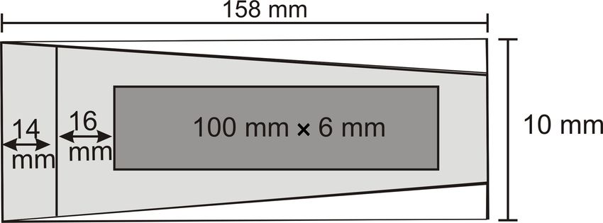
r Figure 1. A two-dimensional cartoon of the different ways of tra-
ditionally dealing with domain edges when computing the radial
where ψi (r) is a count of the number of particles having their distribution function. Panel (a) shows approaches related to a peri-
centers a distance between r − δr and r + δr from the center odic boundary condition approach, whereas (b) illustrates a guard
of the ith particle in the measurement volume, N is the to- area approach.
tal number of particles in the measurement volume, V is the
measurement volume, and dVr is the volume of the general-
3.2 Computing the radial distribution function in
ized n-dimensional shell between radii r − δr and r + δr.
multiple dimensions with periodic boundary
3.1 Computing the radial distribution function in one conditions
dimension
The three-dimensional radial distribution function can be ex-
Calculation of g(r) (or its related quantity, the pair- plicitly computed for cloud droplets in drop-resolving direct
correlation function η(r) ≡ g(r)−1) has been frequently per- numerical simulations. In this context, g(r) can be directly
formed on in situ cloud particle data. Typically, a time series evaluated from Eq. (3) without any modification. The factor
of particle detections is converted to spatial positions along that allows computation of the radial distribution function in
a line utilizing the Taylor frozen-field hypothesis (Saw et al., these scenarios is that the numerical simulations utilize peri-
2012b). Then, Eq. (3) is modified to odic boundary conditions – which extend to the computation
of the radial distribution function itself.
Np (r◦ ) When searching for another cloud droplet separated by
g1-D (r◦ ) = h i , (4)
Nin (r◦ ) + 1
2 (δr) (N − 1) /L scale r◦ − δr < r < r◦ + δr, any part of the “search domain”
2 Nex (r◦ )
outside of the simulation volume can be wrapped back
where detected particle centers are located between 0 and around through the other side of the computational domain.
L, Np (r◦ ) is the number of observed particle centers sepa- Since the underlying simulation typically applies this same
rated by r − δr < r◦ < r + δr, Nin (r◦ ) is the number of ob- wrapping boundary condition to resolve particle–fluid and
served particles detected between r◦ and L − r◦ , and Nex (r◦ ) particle–particle interactions, it is consistent with the physics
is the number of observed particles detected between 0 and of the simulation to search for particle pairs across the bound-
r◦ plus the number of observed particles detected between aries as well.
L − r◦ and L. The factor of 1/2 multiplied by Nex (r◦ ) is suf- A cartoon of this process (shown in two dimensions) can
ficient to account for the edges of the sample volume in the be viewed in Fig. 1a. Some of the circular shell surrounding
one-dimensional case. Since typically r◦
L, this is often the particle in the lower left leaves the measurement volume
simplified to (blue portion). When the data come from a direct numeri-
cal simulation, there are no issues in wrapping this volume
Np (r◦ ) around to the upper left and lower right corners (to the or-
g1-D (r◦ ) ≈ . (5)
2N (N − 1) (δr) /L ange regions), in this case finding an additional particle pair
in the upper left. In an actual experiment, however, it is a mis-
The above formula has been used in most previous exper-
take to argue that the particle in the lower left is correlated to
imental studies computing the radial distribution functions
the particle in the upper left at a length scale of r since they
for cloud droplets. In principle, this result can then be used
are in fundamentally different parts of the flow (i.e., any cor-
to estimate the three-dimensional radial distribution function
relation that does exist is for length scale equal to the non-
following the method outlined in Holtzer and Collins (2002),
periodic distance among the particles usually much greater
though the assumptions of statistical homogeneity over the
than r).
tens to hundreds of kilometers required for obtaining a sta-
tistically significant result may be questionable (Larsen et al.,
2014).
www.atmos-meas-tech.net/11/4261/2018/ Atmos. Meas. Tech., 11, 4261–4272, 2018
4264          M. L. Larsen and R. A. Shaw: A method for computing the three-dimensional radial distribution function

3.3    Computing the radial distribution function in
       multiple dimensions without periodic boundary
       conditions

Unfortunately, the technique described in Fig. 1a is not ap-       Figure 2. Another cartoon of the guard area technique used to es-
propriate for most experimental contexts; detected particles       timate the radial distribution function. Note that the fraction of the
on opposite sides of the sample volume do not “know” about         particles contributing to the sum in Eq. (3) decreases as the aspect
each other in the same way that simulations applying peri-         ratio increases, and no estimate of the radial distribution function
odic boundary conditions do.                                       can be made for any distance larger than half the shortest dimension
   The simplest possible solution, albeit the most drastic, in     of the sample volume (when r ≥ L/2, no “inner” region remains).
trying to estimate the radial distribution function for finite
experimental volumes is to ignore these edge effects entirely.
For the cartoon in Fig. 1a, this would be to merely count the      particles that contribute to the sum in Eq. (3) are only the
one particle detected in the yellow ring and do nothing to ac-     five particles shown inside the central white rectangle. This
count for the blue area at all. Unfortunately, this will cause     problem is even worse in 3-D, and the aspect ratio shown
a computational estimate of g(r) to artificially deviate from      here is not unrealistic.
unity; actual cloud droplets may exist in the blue area and           The guard area approach is a valid approach for finite-
need to be counted in order to prevent artificial underestima-     volume cloud measurements, but it imposes a trade-off: ei-
tion of ψi (r) and therefore underestimation of g(r).              ther most of the volume can be used, but with severely lim-
   Much like in the one-dimensional case, the effects of the       ited maximum r, or the available sample volume is severely
edges sometimes can be small enough to make this a mi-             reduced in order to accommodate a maximum r that is of the
nor concern. When the scale of interest r◦ is much less than       same order as the sample volume linear dimensions. Typi-
the smallest dimension of the sample volume (L), relatively        cally as large a range of r as possible is desired (e.g., in or-
few particles inside the sample volume will have their n-          der to have enough scale range to reliably identify power-law
dimensional spherical shells exit the interior of the measure-     exponents), but the associated reduction in available sample
ment volume. Unfortunately, however, (i) experimental con-         volume makes the method quite susceptible to sampling fluc-
ditions for cloud droplets will require estimation of g(r◦ ) for   tuations. In realistic scenarios in which the entire measure-
r◦ approaching L in order to maximize the evaluated range          ment volume contains only a few hundred to a few thousand
of r, and (ii) the problem becomes more prevalent in higher        particles, sampling considerations make use of the guard area
dimensions and in larger aspect ratios since a larger fraction     technique prohibitively limiting.
of the measurement volume is found close to the boundaries.           Here, we introduce an alternative edge-correction strategy
   As noted earlier, this is a problem that has received atten-    inspired by Ripley (1976, 1977) that we call the “effective
tion for at least 35 years (Ripley, 1982). Perhaps the most        volume” radial distribution function method. This approach
common way to deal with these finite-volume effects is de-         does not rely on the use of a guard area and allows all re-
scribed as “minus sampling” on p. 133 of Stoyan et al. (1995)      tained particles to contribute to the computation of the radial
and illustrated in Fig. 1b. Briefly, one defines a “guard area”    distribution function. We start from a refined expression for
within but along the outermost edges of the sampling vol-          the radial distribution function for length scale rj :
ume. Particles inside this guard area are not considered part
                                                                              N
of the actual sample volume V , but are used to find pairs                    X        ψi (rj )/N
                                                                   g(rj ) =                           .                             (6)
for particles within the central (non-guard) part of the mea-

                                                                                               dVri,j
                                                                              i=1   (N − 1)
surement volume. For example, the particle in the center of                                      V
the red circle in Fig. 1b would count three particles between
r−δr and r+δr, despite having only two particle pairs within          This is very similar to Eq. (3), except we have made the
the white region.                                                  computationally motivated step of discretizing the set of dis-
   Note that R can be either fixed or change with the scale of     tances rj and defined a quantity dVri,j , which is defined as
interest (set R = r◦ when computing g(r◦ ).). The guard area       the portion of the volume with a radius between rj − (δr)j
approach does give an unbiased estimator for g(r), but makes       and rj + (δr)j centered on the ith particle that resides within
sub-optimal use of the data. Two particles within the sample       the measurement volume V . (For example, in Fig. 1a, dVri,j
volume could be separated by scale r◦ − δr < r < r◦ + δr but       for the highlighted particle would be calculated as that area
end up not contributing to the observation, due to the fact that   corresponding to the yellow region.) This depends not only
both particles would be in the guard area. Many of the data        on rj and (δr)j but also on the position of the ith particle.
are lost when using such approaches.                               Thus, within this method, the denominator is not a constant
   Figure 2 shows another cartoon that demonstrates how            and must be explicitly calculated particle by particle.
limiting the guard area approach can be in different contexts.        The challenging part of the method is to find dVri,j ; all
Here, R = r is only slightly smaller than L/2. The “inner”         other parts of the numerical method are the same as have

Atmos. Meas. Tech., 11, 4261–4272, 2018                                                  www.atmos-meas-tech.net/11/4261/2018/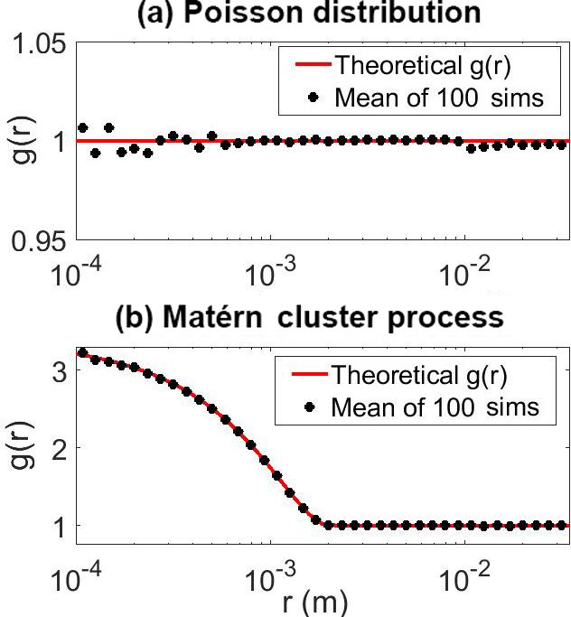
M. L. Larsen and R. A. Shaw: A method for computing the three-dimensional radial distribution function                          4265

been used elsewhere. Although potentially inelegant, dVri,j           4     Testing the effective volume method
can be found for a wide variety of measurement geometries
by generating a measurement geometry-dependent look-up
table. This can be accomplished by computing values of                The effective volume method described above was imple-
dVri,j in a dense grid of possible positions of each detected         mented for two different geometries – a cubical geometry
particle and at each desired distance rj . Since for convex vol-      (to allow for useful comparisons to the well-known and fre-
umes it is empirically found that dVri,j is relatively smooth         quently utilized guard area technique) as well as for an ap-
over the measurement domain, one can then assign dVri,j for           plied geometry to match a real instrument. For each geome-
the ith particle at the j th radial distance by utilizing the look-   try, we present two tests: a homogeneous Poisson distribution
up-table-stored grid point closest to the actual particle posi-       and a Matérn cluster process.
tion.                                                                    A homogeneous Poisson distribution is the gold standard
   There are multiple ways to generate the proposed look-up           of spatial randomness. Within a homogeneous Poisson dis-
table. In this study, we have populated the interior of the mea-      tribution, all particles are placed independently with a spatial
surement volume with a regular dense grid with grid spacing           density function uniform over the measurement domain. By
s. Then, for each grid point and for each scale of interest rj ,      construction, g(r) = 1∀r within a volume with particles dis-
the number of other grid points contained in a shell with in-         tributed according to a homogeneous Poisson distribution.
ner and outer radii rj −(δr)j and rj +(δr)j are counted. This            A Matèrn cluster process (see, e.g., Stoyan et al., 1995;
is then compared to the number of grid points that would be           Martinez and Saar, 2001; Schabenberger and Goway, 2005;
contained in a shell of the same volume within an infinite grid       Larsen, 2012) is commonly used in stochastic geometry be-
with the same grid spacing s. The ratio of these two counts           cause it is (i) statistically homogeneous, (ii) easy to simulate
is then multiplied by the true volume of the shell dVj to give        in any number of spatial dimensions, and (iii) has a known
dVri,j . This method allows for reliable estimation of dVri,j         closed-form expression for its radial distribution function.
without having to mathematically calculate the quantity an-
alytically, which would require rather lengthy treatments of          4.1    Simulations in a cube
possible boundary–shell intersection geometries (especially
in three dimensions).
   Conceptually, the algorithm uses the ith term in the sum           Both distributions described above were simulated within a
in Eq. (6) to find an appropriately weighted contribution to          unit cube with both guard area and effective volume compu-
g(r) from the ith particle; when summed over all particles in         tation methods.
the measurement volume, the expression gives an estimator                For the guard area computation method, a fixed R = 0.1
for g(r) that accounts for edge effects. This weighting fac-          was used around the outside edges of the cube. This should
tor appears in the denominator and is based on a term that            allow for unbiased estimation for g(r) when r < 0.1, but it is
depends on how close the ith particle is to the edge of the           expected that g(r > 0.1) will underestimate the true values.
measurement volume; if the particle in question is within rj             The effective volume computation method was computed
of the edge of the measurement volume, only the portion of            by creating a look-up table for a cubical volume. Due to the
the n-dimensional spherical shell dV that still lies within the       symmetry of the volume, only one octant of the cube had
measurement domain is used.                                           to be included in the look-up table. To minimize the size of
   The effective volume method allows for any investigator-           the look-up table required, the density of the tessellation of
chosen values of rj and (δr)j , allows for as fine of a tessel-       the cubical measurement volume was varied depending on
lation of the measurement volume as desired for precision             the distance to the boundary – with points near the boundary
in the look-up table, and can be used even for rj > L. Once           having the densest collection of look-up table entries.
the look-up table is generated it can be applied to all data             A total of 100 simulations of each volume were averaged
in a data set, assuming the instrument measurement volume             together and the results are displayed in Fig. 3. Except for the
shape and size are constant. It should be further noted that          smallest scales (for which sampling variability is still non-
symmetry in the measurement volume shape can be used to               negligible, even after a total of 100 simulations), agreement
reduce the number of normalization volumes that need to be            between the effective volume method and the theoretical g(r)
calculated. For example, in a rectangular parallelepiped only         curves expected is excellent and comparable to the values
one octant (corner) of the measurement volume needs to be             observed for the more commonly used guard area approach.
in the look-up table. More explicit detail on how to imple-              In this case, the guard area approach involves summing
ment this method is presented in the appendix.                        over less than half (on average 48.8 %) of particles in the
                                                                      measurement volume, which can help to explain the larger
                                                                      scatter of observed g(r) for small r using this approach. Note
                                                                      also the deviation from the theoretical g(r) curve in both tests
                                                                      for the guard area approach for r > 0.1, consistent with push-
                                                                      ing the approach beyond its domain of applicability.

www.atmos-meas-tech.net/11/4261/2018/                                                   Atmos. Meas. Tech., 11, 4261–4272, 2018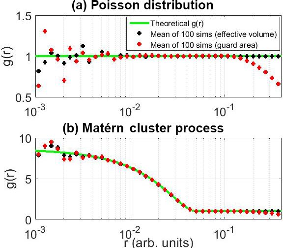
4266           M. L. Larsen and R. A. Shaw: A method for computing the three-dimensional radial distribution function

                                                                       Figure 4. A two-dimensional cartoon of the HOLODEC sample
                                                                       volume (not to scale). The leftmost vertical line in the figure in-
                                                                       dicates the hologram plane. The light grey region indicates areas
                                                                       of maximum sensor sensitivity (the slope of the angled lines mark-
                                                                       ing the edge of the light grey region has been greatly magnified
                                                                       for aid in visualization). The vertical lines 14 and 158 mm from
                                                                       the left edge of the figure mark the positions of the optical win-
                                                                       dows; near these windows there is evidence of artificially generated
                                                                       particles due to instrument-induced particle fragmentation. The vol-
                                                                       ume simulated here corresponds to the darker central grey rectangle
                                                                       (parallelepiped in 3-D), where the instrument retains approximately
                                                                       uniform sensitivity, particle locations and sizes are believed to be
                                                                       accurate, and the number of small particles generated due to frag-
                                                                       mentation on the instrument is believed to be negligible.
Figure 3. First verification of the method for calculating g(r) de-
scribed in the main text. Here, theoretical curves of g(r) are com-
pared to both the effective volume method and the guard area
method (using a fixed guard area of 0.1 times the side length of the   instrument has been validated by comparison to co-collected
cube). In the top panel, 100 different 10 000 particle Poisson dis-    cloud droplet probe (CDP) and 2DC optical array probe data
tributions were created. Deviations from g(r) = 1 in both methods      in different parts of the particle size domain (Glienke et al.,
are observed at small r values due to sampling fluctuations. Panel     2017).
(b) shows similar results from 100 simulations of a Matérn cluster        A      processed      HOLODEC          hologram      reports
process (with a mean of 10 000 total particles and a cluster length    droplet positions in a volume that is approximately
of 0.025). Note that in both panels the guard area approach begins     1 cm × 1 cm × 15.8 cm with sensitivity to all droplets with
to fail as expected for r > 0.1.                                       sizes greater than about 6.5 µm. The positional uncertainty
                                                                       for each drop is approximately 10 µm along the short sides
                                                                       of the sample volume and about 100 µm along the longer
4.2     Case study: the Holographic Detector for Clouds                side (Yang et al., 2005).
        (HOLODEC)                                                         A two-dimensional cartoon of the HOLODEC sample vol-
                                                                       ume is shown in Fig. 4. Although particles out to 158 mm
Although the effective volume approach introduced here per-            (or further) from the hologram plane are potentially visi-
forms approximately as well as the more traditional guard              ble, the optical windows 14 and 158 mm from the hologram
area approach in cubical volumes, the development of the               plane limit the air-exposed field of view to the approximately
new method was primarily motivated by a desire to estimate             14 cm distance between the windows. Additionally, the spa-
the radial distribution function in contexts in which the guard        tial domain of instrumental sensitivity is not a perfect par-
area approach will not work. As noted previously, when es-             allelepiped. Preliminary analyses of data suggest that there
timates of g(r) are desired for r&L/2 and/or the aspect ra-            may be some decreased sensitivity near the edges of the
tio of the measurement volume deviates substantially from              sample volume, and – when mounted on an aircraft – drops
unity, the guard area approach becomes ineffective.                    can be created by fragmentation near the optical windows
   An example of an instrument that is subject to these lim-           (Fugal and Shaw, 2009). Consequently, to ensure data fi-
itations and is relevant for studying cloud particle clustering        delity when used with real data, a conservative sub-volume
is the Holographic Detector for Clouds (HOLODEC).                      of each hologram is selected as the measurement volume for
                                                                       analysis. This sub-volume was selected to be in the central
4.2.1    Introduction to HOLODEC                                       part of each hologram where the data are expected to be
                                                                       most reliable. Thus, the used HOLODEC sample volume is
HOLODEC is an in-line digital holography instrument ex-                a 6 mm × 6 mm × 10 cm rectangular parallelepiped.
plicitly designed to explore cloud microstructure (Fugal
et al., 2004; Fugal and Shaw, 2009; Spuler and Fugal, 2011).           4.2.2   Simulations within the instrument domain
The instrument has previously been used to examine drop
size distribution and liquid water content fluctuations on the         The same two tests (homogeneous Poisson distribution and
centimeter scale (Beals et al., 2015), and the behavior of the         Matérn cluster process) were simulated within the paral-

Atmos. Meas. Tech., 11, 4261–4272, 2018                                                   www.atmos-meas-tech.net/11/4261/2018/
M. L. Larsen and R. A. Shaw: A method for computing the three-dimensional radial distribution function 4267
Figure 5. Verification that the effective volume method for calculat-
ing g(r) as described in the main text works for non-cubical sample Figure 6. The measured radial distribution functions for eight dif-
volumes with realistic aspect ratios. In panel (a), 100 different sim- ferent holograms and their mean for HOLODEC data taken in the
ulations of a Poisson distribution (perfect spatial randomness) were cloud chamber. Clearly sampling variability is still pronounced at
created by placing 10 000 particles within a sample volume with the small spatial scales, but some evidence of scale-dependent cluster-
same dimensions as the HOLODEC sample volume. The mean of ing seems possible.
the 100 simulations agrees very well with the theoretical g(r) = 1
curve. An unrealistically large number of particles were used for
each simulation in order to minimize the sampling concerns. Note
that though the agreement is very good, the most pronounced de- surement domain (which is reasonable compared to naturally
viations from the theoretical curve still occur as expected at small occurring clouds).
spatial scales. In panel (b), 100 different simulations of a Matérn These single-hologram results are noisy due to the sam-
cluster process were generated and compared to the known theoret- pling uncertainty (especially for the smallest spatial scales),
ical expression (see, e.g., Larsen et al., 2014). Clearly, agreement but it is clear that there is some evidence of scale-dependent
between the mean of the simulations and the theoretical curve is
clustering revealed for r.1 mm. Quantitative comparisons to
excellent.
theoretical expectation are too much to ask for from such
a limited data set, but it is promising to note that the g(r)
curve decays as expected to unity for scales larger than a
lelepiped sample volume of the HOLODEC. A new look- few η (where η is the turbulent Kolmogorov scale – nomi-
up table for this geometry was generated and used to cal- nally 1 mm for the atmosphere). Additionally, the observed
culate g(r) for each of 100 different simulations, with the increase in g(r) with decreasing length scale r within the
mean value of g(r) compared to theoretical expectations and dissipative range is consistent with expectations for inertial
shown in Fig. 5. The guard area method for calculating g(r) clustering of particles in a turbulent flow (Reade and Collins,
is not shown since it is susceptible to substantial sampling 2000; Ayala et al., 2008; Saw et al., 2012a). Despite these en-
variability at all scales and cannot be used at all for any scale couraging features, it is important to note that here we merely
larger than 3 mm (the entire volume is then the guard area). present Fig. 6 to demonstrate that the algorithm gives plausi-
In general, the agreement between the theoretical expres- ble results for real data; quantitative analysis of these cham-
sions for g(r) and the measured g(r) is excellent, and sug- ber data with so few holograms would be premature.
gests that the effective volume radial distribution function Actually measuring the three-dimensional radial distribu-
computational method should work for real data. tion function for in situ flight data will still be challenging,
even with the aid of the algorithm introduced here. The ra-
4.2.3 Real data dial distribution function curves shown in Fig. 6 suggest that
individual holograms likely do not give statistically reliable
To test the claim made above, a proof-of-principle analysis information on spatial scales of microphysical interest; thus
was completed using real HOLODEC data acquired inside a some means of combining information from multiple holo-
laboratory cloud chamber driven by Rayleigh–Bénard con- grams will need to be explored in the future. The number
vection (Chandrakar et al., 2016, 2017; Chang et al., 2016; of holograms needed for extraction of in situ radial distribu-
Desai et al., 2018). tion function values will critically depend on data and instru-
The radial distribution functions of the eight holograms ment parameters including (i) the spatial scale of interest (r),
with the largest numbers of detected drops are shown in (ii) the spatial resolution of interest (dr), (iii) the size and
Fig. 6. For these eight holograms, there were an average of shape of the measurement volume of the instrument, (iv) the
about 185 cloud drops per cubic centimeter within the mea- density of cloud particles, and (v) the acceptable level of un-
www.atmos-meas-tech.net/11/4261/2018/ Atmos. Meas. Tech., 11, 4261–4272, 20184268 M. L. Larsen and R. A. Shaw: A method for computing the three-dimensional radial distribution function
certainty in the extracted radial distribution function. For ex- Comparing measurements with theory and numerical sim-
ample, a crude estimate with fixed dr = 100 µm for the data ulation relies on estimating g(r) over a wide range of spa-
presented here suggests that estimation to within 1 % uncer- tial scales and making optimal use of the measured data
tainty in g(r) requires only one hologram for reliable estima- to combat sampling uncertainties. Because the aspect ratios
tion of g(r = 1 cm) but approximately 60 holograms for reli- of the holographic instruments designed to explore three-
able estimation of g(r = 1 mm) and almost 3000 holograms dimensional cloud microstructure are large and the radial
for reliable estimation of g(r = 100 µm). However, the num- distribution function must be estimated on scales exceeding
ber of required holograms may be more modest depending on the smallest dimension of the measurement volume, standard
the drop number concentration, usable measurement volume computational methods that use spatial information to esti-
of the sensor, scale of physical interest, spatial resolution of mate the radial distribution function are not adequate.
g(r) required, and/or the level of acceptable uncertainty in Here, a new method was introduced that explicitly con-
the estimate of g(r). Current work with in situ data has re- siders each particle’s position within the measurement vol-
vealed promising results, but here our emphasis has been on ume in the radial distribution function computation. This
proving the viability of the numerical algorithm. method allows for calculating the radial distribution func-
tion for scales larger than the shortest physical dimension
of the measurement volume and makes more optimal use of
5 Conclusions the measured data. This effective volume method was tested
in two different geometries, compared to standard computa-
Understanding the effects of cloud particle clustering on
tional methods with simulated data in a unit cube, and vali-
microphysical processes requires reliable estimation of
dated in a more realistic sampling scenario.
the three-dimensional radial distribution function. Previous
Preliminary results confirm that use of the effective vol-
studies have obtained this information by utilizing one-
ume method should enable the use of airborne digital holog-
dimensional measurements of cloud particle positions to in-
raphy data to compute in situ three-dimensional radial distri-
fer scale-dependent clustering, but these methods have been
bution functions for cloud droplets.
shown to carry large uncertainties. In the hope of finding
an alternative way of characterizing cloud particle clustering
without such restrictive underlying assumptions and/or un- Data availability. The HOLODEC data associated with the analy-
certainties, measurement of the radial distribution function sis in Sect. 4.2.3 are available from the authors by request.
for in situ data in three dimensions is desired.
Atmos. Meas. Tech., 11, 4261–4272, 2018 www.atmos-meas-tech.net/11/4261/2018/M. L. Larsen and R. A. Shaw: A method for computing the three-dimensional radial distribution function 4269
Appendix A: Basic structure of codes to use the effective A2 Using the look-up table and data to compute a
volume method radial distribution function
The effective volume method to calculate the radial distribu- Required inputs include the same set of inputs utilized to gen-
tion function relies on two codes – one to generate a look- erate the look-up table and N different n-dimensional parti-
up table for the measurement volume, and another to use cle positions.
the look-up table and data to compute the radial distribution
function. This appendix outlines the basic structure utilized 1. Load the look-up table.
for each of these codes.
2. For each radius rj , calculate the volume of the n-
A1 Generating the look-up table dimensional spherical shell between radii rj −(δr)j and
rj + (δr)j . Store the results as dV (j ).
Required inputs from the user include the following: physi-
3. For each particle k = 1 : N and for each radius rj
cal domain of sample volume, set of radii rj and associated
ranges (δr)j , and grid tessellation scale s (as small as com- (a) count the number of other particles that are between
putationally feasible). rj − (δr)j and rj + (δr)j from the kth particle and
store the result as ψ(k, j ).
1. Tessellate the interior of the sample volume domain at
scale s, giving a total of M grid points. (b) identify the closest entry in the look-up table i to
the associated position of the kth particle; store as
2. For each radius rj , and for each grid point i = 1 : p.
M, compute the number of grid points inside the n- (c) assign dV r(k, j ) = dV (j ) · norm(p, j ) .
dimensional shell centered on the ith grid point with
inner and outer radii rj − (δr)j and rj + (δr)j , respec- (d) use dV r(k, j ) and ψ(k, j ) to compute the kth term
tively. Store the result as a(i, j ). of the sum for g(r) following Eq. (6) to give
g(k, j ).
3. Tessellate an n-dimensional
cube at scale s with side 4. Compute and return g(j ) = N
P
lengths 2 max rj + (δrj ) . k=1 g(k, j ).
4. For each radius rj , compute the number of grid points
inside the n-dimensional shell centered on the center
of the n-dimensional cube with inner and outer radii
rj − (δr)j and rj + (δr)j , respectively. Store the result
as b(j ).
5. Compute the factor norm(i, j ) = a(i, j )/b(j ).
www.atmos-meas-tech.net/11/4261/2018/ Atmos. Meas. Tech., 11, 4261–4272, 20184270 M. L. Larsen and R. A. Shaw: A method for computing the three-dimensional radial distribution function
Competing interests. The authors declare that there is no conflict of Chaumat, L. and Brenguier, J.: Droplet spectra broadening in cu-
interest. mulus clouds. Part II: Microscale droplet concentration inhomo-
geneities, J. Atmos. Sci., 58, 642–654, 2001.
Cherkas, N. and Cherkas, S.: Model of the radial distribution func-
Acknowledgements. This work was supported by the US National tion of pores in a layer of porous aluminum oxide, Crystallogr.
Science Foundation through grants AGS-1532977 (MLL) and Rep., 61, 285–290, 2016.
AGS-1623429 (RAS). Special thanks to Alexander Kostinski, Chun, J., Koch, D., Rani, S., Ahluwalia, A., and Collins, L.: Clus-
Susanne Glienke, and Neel Desai for helpful discussions and help tering of aerosol particles in isotropic turbulence, J. Fluid Mech.,
with accessing and interpreting the HOLODEC data from the 5 536, 219–251, 2005.
Chamber. Collins, L. and Keswani, A.: Reynolds number scaling of particle
clustering in turbulent aerosols, New J. Phys., 6, 1–17, 2004.
Edited by: Szymon Malinowski Conway, B., Caughey, S., Bentley, A., and Turton, J.: Ground-based
Reviewed by: three anonymous referees and airborne holography of ice and water clouds, Atmospheric
Environment, 16, 1193–1207, 1982.
Davis, A., Marshak, A., Gerber, H., and Wiscombe, W.: Horizon-
tal structure of marine boundary layer clouds from centimeter to
kilometer scales, J. Geophys. Res., 104, 6123–6144, 1999.
References Desai, N., Chandrakar, K., Chang, K., Cantrell, W., and Shaw, R.:
Influence of microphysical variability on stochastic condensa-
Ayala, O., Rosa, B., Wang, L.-P., and Grabowski, W.: Effects tion in a turbulent laboratory cloud, J. Atmos. Sci., 75, 189–201,
of turbulence on the geometric collision rate of sediment- 2018.
ing droplets. Part I: Results from direct numerical simula- Erimbetova, L., Davletov, A., Kudyshev, Z. A., and Mukhametkari-
tion, New J. Phys., 10, 075015, https://doi.org/10.1088/1367- mov, Y. S.: Influence of polarization phenomena on radial distri-
2630/10/7/075015, 2008. bution function of dust particles, Contrib. Plasm. Phys., 53, 414–
Baker, B.: Turbulent entrainment and mixing in clouds: A new ob- 418, 2013.
servational approach, J. Atmos. Sci., 49, 387–404, 1992. Frankel, A., Iaccarino, G., and Mani, A.: Optical depth in particle-
Baker, B. and Lawson, R.: Analysis of tools used to quantify droplet laden turbulent flows, J. Quant. Spesc. Ra., 201, 10–16, 2017.
clustering in clouds, J. Atmos. Sci., 67, 3355–3367, 2010. Fugal, J. P. and Shaw, R. A.: Cloud particle size distributions mea-
Balkovsky, E., Falkovich, G., and Fouxon, A.: Intermittent distribu- sured with an airborne digital in-line holographic instrument,
tion of inertial particles in turbulent flows, Phys. Rev. Lett., 86, Atmos. Meas. Tech., 2, 259-271, https://doi.org/10.5194/amt-2-
2790–2793, 2001. 259-2009, 2009.
Bateson, C. and Aliseda, A.: Wind tunnel measurements of the Fugal, J., Shaw, R., Saw, E.-W., and Sergeyev, A.: Airborne dig-
preferential concentration of inertial droplets in homogenous ital holographic system for cloud particle measurements, Appl.
isotropic turbulence, Exp. Fluids, 52, 1373–1387, 2012. Optics, 43, 5987–5995, 2004.
Baumgardner, D., Baker, B., and Weaver, K.: A technique fo rthe Glienke, S., Kostinski, A., Fugal, J., Shaw, R., Borrmann, S.,
measurements of cloud structure in centimeter scales, J. Atmos. and Stith, J.: Cloud droplets to drizzle: Contribution of tran-
Ocean. Technol., 10, 557–565, 1993. sition drops to microphysical and optical properties of ma-
Beals, M., Fugal, J., Shaw, R., Lu, J., Spuler, S., and Stith, J.: Holo- rine stratocumulus clouds, Geophys. Res. Lett., 44, 8002–8010,
graphic measurements of inhomogeneous cloud mixing at the https://doi.org/10.1002/2017GL074430, 2017.
centimeter scale, Science, 350, 87–90, 2015. Holtzer, G. and Collins, L.: Relationship between the intrinsic ra-
Borrmann, S., Jaenicke, R., and Neumann, P.: On spatial distribu- dial distribution function for an isotropic field of particles and
tions and inter-droplet distances measured in stratus clouds with lower-dimensional measurements, J. Fluid Mech., 459, 93–102,
in-line holography, Atmos. Res., 29, 229–245, 1993. https://doi.org/10.1017/S0022112002008169, 2002.
Brenguier, J.-L.: Observations of cloud microstructure at the cen- Jackson, R., McFarquhar, G., Stith, J., Beals, M., Shaw, R., Jensen,
timeter scale, J. Appl. Meteorol., 32, 783–793, 1993. J., Fugal, J., and Korolev, A.: An assessment of the impact of an-
Brown, P.: Use of holography for airborne cloud physics measure- tishattering tips and artifact removal techniques on cloud ice size
ments, J. Atmos. Ocean. Technol., 6, 293–306, 1989. distributions measured by the 2D cloud probe, J. Atmos. Ocean.
Chandrakar, K., Cantrell, W., Chang, K., Ciochetto, D., Nieder- Technol., 31, 2567–2590, 2014.
meier, D., Ovchinnikov, M., Shaw, R., and Yang, F.: Aerosol indi- Kostinski, A.: On the extinction of radiation by a homogeneous but
rect effect from turbulence-induced broadening of cloud-droplet spatially correlated random medium, J. Opt. Soc. Am. A, 18,
size distributions, P. Natl. Acad. Sci., 113, 14243–14248, 2016. 1929–1933, https://doi.org/10.1364/JOSAA.18.001929, 2001.
Chandrakar, K., Cantrell, W., Ciochetto, D., Karki, S., Kinney, G., Kostinski, A.: Simple approximations for condensational growth,
and Shaw, R.: Aerosol removal and cloud collapse accelerated by Environ. Res. Lett., 4, 015005, https://doi.org/10.1088/1748-
supersaturation fluctuations in turbulence, Geophys. Res. Lett., 9326/4/1/015005, 2009.
44, 4359–4367, 2017. Kostinski, A. and Jameson, A.: On the spatial distribution of cloud
Chang, K., Bench, J., Brege, M., Cantrell, W., Chandrakar, K., Cio- particles, J. Atmos. Sci., 57, 901–915, 2000.
chetto, D., Mazzoleni, C., Mazzoleni, L., Niedermeier, D., and Kostinski, A. and Shaw, R.: Scale-dependent droplet clustering in
Shaw, R.: A laboratory facility to study gas-aerosol-cloud inter- turbulent clouds, J. Fluid Mech., 434, 389–398, 2001.
actions in a turbulent enviornment: The 5 chamber, B. Am. Me-
teor. Soc., 97, 2343–2358, 2016.
Atmos. Meas. Tech., 11, 4261–4272, 2018 www.atmos-meas-tech.net/11/4261/2018/M. L. Larsen and R. A. Shaw: A method for computing the three-dimensional radial distribution function 4271 Kozikowsa, A., Haman, K., and Supronowicz, J.: Preliminary re- Saw, E.-W., Shaw, R., Ayyalasomayajula, S., Chuang, P., and sults of an investigation of the spatial distribution of fog droplets Gylfason, A.: Inertial particle clustering of particles in high- by a holographic method, Q. J. Roy. Meteorol. Soc., 110, 65–73, Reynolds-number turbulence, Phys. Rev. Lett., 100, 214501, 1984. https://doi.org/10.1103/PhysRevLett.100.214501, 2008. Landau, L. and Lifshitz, E.: Statistical Physics, Butterworth Heine- Saw, E.-W., Salazar, J., Collins, L., and Shaw, R.: Spatial clus- mann, Oxford, UK, 1980. tering of polydisperse inertial particles in turbulence: I. Com- Larsen, M.: Studies of discrete fluctuations in atmospheric phenom- paring simulation with theory, New J. Phys., 14, 105030, ena, Ph.D. thesis, Michigan Technological University, 2006. https://doi.org/10.1088/1367-2630/14/10/105030, 2012a. Larsen, M.: Scale localization of cloud particle clustering statistics, Saw, E.-W., Shaw, R., Salazar, J., and Collins, L.: Spatial clus- J. Atmos. Sci., 69, 3277–3289, https://doi.org/10.1175/JAS-D- tering of polydisperse inertial particles in turbulence: II. Com- 12-02.1, 2012. paring simulation with experiment, New J. Phys., 14, 105031, Larsen, M., Briner, C., and Boehner, P.: On the recovery of 3D spa- https://doi.org/10.1088/1367-2630/14/10/105031, 2012b. tial statistics of particles from 1D measurements: Implications Schabenberger, O. and Goway, C.: Statistical Methods for Spatial for airborne instruments, J. Atmos. Ocean. Technol., 31, 2078– Data Analysis, Chapman and Hall/CRC, Boca Raton, 504 pp., 2087, https://doi.org/10.1175/JTECH-D-14-00004.1, 2014. 2005. Lee, K. and Seong, W.: Percus-Yevick radial distribution function Schlenczek, O., Fugal, J., Lloyd, G., Bower, K., Choularton, T., calculation for a water-saturated granular medium, Ocean Eng., Flynn, M., Crosier, J., and Borrmann, S.: Microphysical proper- 116, 268–272, 2016. ties of ice crystal precipitation and surface-generated ice crystals Lehmann, K., Siebert, H., Wendisch, M., and Shaw, R.: Evidence in a high alpine environment in Switzerland, J. Appl. Meteorol. for inertial droplet clustering in weakly turbulent clouds, Tellus, Climatol., 56, 433–453, 2017. 59B, 57–65, 2007. Shaw, R.: Particle-turbulence interactions in atmo- Marshak, A., Knyazikhin, Y., Larsen, M., and Wiscombe, W. J.: spheric clouds, Annu. Rev. Fluid Mech., 35, 183–227, Small-scale drop size variability: Empirical models for drop- https://doi.org/10.1146/annurev.fluid.35.101101.161125, 2003. size-dependent clustering in clouds, J. Atmos. Sci., 62, 551–558, Shaw, R., Reade, W., Collins, L., and Verlinde, J.: Preferential con- 2005. centration of cloud droplets by turbulence: Effects on the early Martinez, V. and Saar, E.: Statistics of the Galaxy Distribution, CRC evolution of cumulus cloud droplet spectra, J. Atmos. Sci., 55, Press, Boca Raton, 456 pp., 2001. 1965–1976, 1998. Monchaux, R., Bourgoin, M., and Cartellier, A.: Analyzing prefer- Shaw, R., Kostinski, A., and Larsen, M.: Towards quantify- ential concentration and clustering of inertial particles in turbu- ing droplet clustering in clouds, Q. J. Roy. Meteorol. Soc., lence, Int. J. Multiphas. Flow, 40, 1–18, 2012. 128, 1043–1057, https://doi.org/10.1256/003590002320373193, Onishi, R., Matsuda, K., and Takahashi, K.: Lagrangian tracking 2002. simulation of droplet growth in turbulence – Turbulence en- Siebert, H., Gerashchenko, S., Gylfason, A., Lehmann, K., Collins, hancement of autoconversion rate, J. Atmos. Sci., 72, 2591– L., Shaw, R., and Warhaft, Z.: Towards understanding the role of 2607, 2015. turbulence on droplets in clouds: In situ and laboratory measure- Ornstein, L. and Zernike, F.: Accidental deviations of density and ments, Atmos. Res., 97, 426–437, 2010. opalescence at the critical point of a single substance, KNAW Siebert, H., Shaw, R. A., Ditas, J., Schmeissner, T., Malinowski, S. Proc., 17, 793–806, 1914. P., Bodenschatz, E., and Xu, H.: High-resolution measurement O’Shea, S., Choularton, T., Lloyd, G., Crosier, J., Bower, K., Gal- of cloud microphysics and turbulence at a mountaintop station, lagher, M., Abel, S., Cotton, R., Brown, P., Fugal, J., Schlenczek, Atmos. Meas. Tech., 8, 3219–3228, https://doi.org/10.5194/amt- O., Borrmann, S., and Pickering, J.: Airborne observations of the 8-3219-2015, 2015. microphysical structure of two contrasting cirrus clouds, J. Geo- Small, J. and Chuang, P.: New observations of precipitation initi- phys. Res.-Atmos., 121, 13510–13536, 2016. ation in warm cumulus clouds, J. Atmos. Sci., 65, 2972–2982, Pinsky, M. and Khain, A.: Fine structure of cloud droplet concen- 2008. tration as seen from the Fast-FSSP measurements. Part I: Method Spuler, S. and Fugal, J.: Design of an in-line, digital holographic of analysis and preliminary results, J. Appl. Meteorol., 40, 1515– imaging system for airborne measurement of clouds, Appl. Op- 1537, 2001. tics, 50, 1405–1412, 2011. Reade, W. and Collins, L.: Effect of preferential concentration on Srivastava, R.: Growth of cloud drops by condensation: A criticism turbulent collision rates, Phys. Fluids, 12, 2530–2540, 2000. of currently-accepted theory and a new approach, J. Atmos. Sci., Ripley, B.: The second-order analysis of stationary point processes, 46, 869–887, 1989. J. Appl. Probab., 13, 255–266, 1976. Stoyan, D., Kendall, W., and Mecke, J.: Stochastic Geometry and Ripley, B.: Modelling spatial paterns (with discussion), J. Roy. Stat. its Applications, Wiley, Chichister, England, 436 pp., 1995. Soc., B39, 172–212, 1977. Uhlig, E.-M., Borrmann, S., and Jaenicke, R.: Holographic in-situ Ripley, B.: Edge effects in spatial stochastic processes, in: Statistics measurements of the spatial droplet distribution in stratiform in Theory and Practice: Essays in Honour of Bertil Matérn, edited clouds, Tellus, 50B, 377–387, 1998. by: Ranneby, B., 242–262, 1982. Wang, L., Wexler, A., and Zhou, Y.: Statistical mechanical descrip- Salazar, J., Jong, J. D., Cao, L., Woodward, C., Meng, H., and tion and modeling of trubulent collision of inertial particles, J. Collins, L.: Experimental and numerical inverstigation of inertial Fluid Mech., 415, 117–153, 2000. particle clustering in isotropic turbulence, J. Fluid Mech., 600, 245–256, 2008. www.atmos-meas-tech.net/11/4261/2018/ Atmos. Meas. Tech., 11, 4261–4272, 2018
4272           M. L. Larsen and R. A. Shaw: A method for computing the three-dimensional radial distribution function

Xue, Y., Wang, L.-P., and Grabowski, W.: Growth of cloud droplets        Zaichik, L. and Alipchenkov, V.: Statistical models for predict-
  by turbulent collision-coalescence, J. Atmos. Sci., 65, 331–356,         ing pair dispersion and particle clustering in isotropic tur-
  2008.                                                                    bulence and their applications, New J. Phys., 11, 103018,
Yang, W., Kostinski, A., and Shaw, R.: Depth-of-focus reduction for        https://doi.org/10.1088/1367-2630/11/10/103018, 2009.
  digital in-line holography of particle fields, Opt. Lett., 30, 1303–
  1305, 2005.

Atmos. Meas. Tech., 11, 4261–4272, 2018                                                    www.atmos-meas-tech.net/11/4261/2018/
You can also read