The SPIRou wavelength calibration for precise radial velocities in
←
→
Page content transcription
If your browser does not render page correctly, please read the page content below
Astronomy & Astrophysics manuscript no. main                                                                                       ©ESO 2021
                                              February 5, 2021

                                                The SPIRou wavelength calibration for precise radial velocities in
                                                                   the near infrared?,??
                                                    M. J. Hobson1, 2 , F. Bouchy3 , N. J. Cook4 , E. Artigau4 , C. Moutou5, 6 , I. Boisse1 , C. Lovis3 , A. Carmona7 , X.
                                                                                     Delfosse7 , J.-F. Donati5 , and the SPIRou Team

                                                    1
                                                        Aix Marseille Univ, CNRS, CNES, LAM, Marseille, France
                                                        e-mail: mhobson@astro.puc.cl
                                                    2
                                                        Millennium Institute for Astrophysics, Chile
                                                    3
                                                        Observatoire Astronomique de l’Université de Genève, 51 Chemin des Maillettes, 1290 Versoix, Switzerland
                                                    4
                                                        Institut de Recherche sur les Exoplanètes (IREx), Département de Physique, Université de Montréal, C.P. 6128, Succ. Centre-Ville,
arXiv:2102.02324v1 [astro-ph.IM] 3 Feb 2021

                                                        Montréal, QC, H3C 3J7, Canada
                                                    5
                                                        Univ. de Toulouse, CNRS, IRAP, 14 avenue Belin, 31400 Toulouse, France
                                                    6
                                                        Canada-France-Hawaii Telescope Corporation, 65-1238 Mamalahoa Hwy, Kamuela, HI 96743, USA
                                                    7
                                                        Univ. Grenoble Alpes, CNRS, IPAG, 38000 Grenoble, France
                                                    Received 13 May 2020, accepted 18 January 2021

                                                                                                                 ABSTRACT

                                                    Aims. SPIRou is a near-infrared (nIR) spectropolarimeter at the CFHT, covering the YJHK nIR spectral bands (980 − 2350 nm). We
                                                    describe the development and current status of the SPIRou wavelength calibration in order to obtain precise radial velocities (RVs) in
                                                    the nIR.
                                                    Methods. We make use of a UNe hollow-cathode lamp and a Fabry-Pérot étalon to calibrate the pixel-wavelength correspondence for
                                                    SPIRou. Different methods are developed for identifying the hollow-cathode lines, for calibrating the wavelength dependence of the
                                                    Fabry-Pérot cavity width, and for combining the two calibrators.
                                                    Results. The hollow-cathode spectra alone do not provide a sufficiently accurate wavelength solution to meet the design requirements
                                                    of an internal error of < 0.45 m s−1 , for an overall RV precision of 1 m s−1 . However, the combination with the Fabry-Pérot spectra
                                                    allows for significant improvements, leading to an internal error of ∼ 0.15 m s−1 . We examine the inter-night stability, intra-night
                                                    stability, and impact on the stellar RVs of the wavelength solution.
                                                    Key words. Astronomical instrumentation, methods and techniques – Instrumentation: spectrographs

                                              1. Introduction                                                                Historically, two main instrumental approaches have been
                                                                                                                         used for wavelength calibration: iodine cells and hollow-cathode
                                              The spectroscopic method of exoplanet detection, also known as             (HC) lamps. Each of these calibrators has advantages and disad-
                                              the radial velocity (RV) method, has proven itself extremely pro-          vantages. With iodine cells, the calibrating spectrum is imprinted
                                              ductive, with over 700 exoplanets discovered by this method1 .             directly on the stellar spectrum, allowing for a fully simultane-
                                              The detection of exoplanets through spectroscopy relies on the             ous calibration (e.g. Marcy & Butler 1992; Butler et al. 1996).
                                              extremely precise measurement of tiny shifts of the stellar spec-          However, the iodine lines span only a small portion of the op-
                                              tral lines. In order to make these measurements, a precise wave-           tical spectrum (around 510 to 620 nm, Fischer et al. 2016), and
                                              length solution is in turn required.                                       a high signal-to-noise ratio (S/N) is required to model the line
                                                                                                                         spread function. With HC lamps (primarily ThAr in the visi-
                                                 ?
                                                                                                                         ble), calibration exposures must be taken before the stellar ob-
                                                   Based on observations obtained at the Canada-France-Hawaii Tele-      servations, and a separate fibre is required to monitor the in-
                                              scope (CFHT), which is operated from the summit of Maunakea by             strument drift from the time of calibration (e.g. Baranne et al.
                                              the National Research Council of Canada, the Institut National des
                                                                                                                         1996). The advantage of these lamps is that the thorium lines
                                              Sciences de l’Univers of the Centre National de la Recherche Scien-
                                              tifique of France, and the University of Hawaii. The observations at the   cover a much larger wavelength domain than the iodine lines,
                                              Canada-France-Hawaii Telescope were performed with care and respect        and - as they are not superimposed on the stellar spectrum -
                                              from the summit of Maunakea which is a significant cultural and his-       fainter targets can be observed. An overview of the main spec-
                                              toric site. Based on observations obtained with SPIRou, an international   trographs operating in the visible, their wavelength calibrators,
                                              project led by Institut de Recherche en Astrophysique et Planétologie,     and measurement precisions, is given in Fischer et al. (2016).
                                              Toulouse, France.                                                          For iodine cells, the precision is limited to ≈ 1 m s−1 (Fischer
                                               ??
                                                   Table A1 is only available in electronic form at the CDS via anony-   et al. 2016, Spronck et al. 2015). As for the ThAr HC lamps,
                                              mous ftp to cdsarc.u-strasbg.fr (130.79.128.5) or via http://cdsweb.u-     Lovis & Pepe (2007) were able to achieve a groundbreaking
                                              strasbg.fr/cgi-bin/qcat?J/A+A/                                             20 cm s−1 precision for the wavelength solution of the HARPS
                                               1
                                                  See e.g. The Exoplanets Encyclopaedia (http://exoplanet.eu/),
                                                                                                                         spectrograph through the creation of an improved line list. For
                                              the NASA Exoplanet Archive (https://exoplanetarchive.ipac.
                                              caltech.edu/).                                                             the near-infrared (nIR), however, HC lamps alone limit preci-

                                                                                                                                                                   Article number, page 1 of 12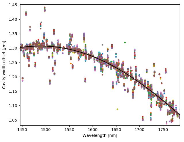
A&A proofs: manuscript no. main

sion to above 1 m s−1 (Halverson et al. 2014), and the fill gases       a given polarisation state, either circular or linear), and one for
emit bright lines that saturate the detectors (Quirrenbach et al.       calibration.
2018).                                                                       The SPIRou calibration unit has been previously described in
    In order to increase the precision of the wavelength solu-          Boisse et al. (2016), and Perruchot et al. (2018). The calibration
tion and enable the detection of smaller planets, Fabry-Pérot           module permits the illumination of science, calibration, or all
(FP) étalons and laser frequency combs (LFCs) have recently             channels simultaneously, by any of the following: a cold source
begun to be incorporated into wavelength solutions. Fabry-Pérot         (Black Acktar surface at -25 ◦ C) for observation of faint stars
étalons provide lines that are evenly spaced in frequency, but          without simultaneous calibration; a white lamp (Tg) for blaze
whose wavelengths need to be derived by anchoring to an abso-           measurement; one of two HC lamps, UNe or ThAr, for wave-
lute calibrator, such as an HC lamp (e.g. Bauer et al. 2015). As        length calibration; an FP étalon for wavelength calibration and
an example, the HARPS spectrograph can achieve 10 cm s−1 pre-           simultaneous drift monitoring; or a reserve port intended for fu-
cision over one night through the incorporation of the FP lines         ture upgrades or visitor instruments.
(Wildi et al. 2011). Likewise, the CARMENES spectrograph in-                 The wavelength calibrators are the HC lamps and the FP
corporates FP observations into the wavelength calibrations for         étalon. Figures 1 and 2 show the central regions of raw SPIRou
both its visible and nIR arms; for the nIR arm especially, it is a      spectra of the UNe lamp and the FP étalon, respectively. Each
necessity due to the less densely populated emission lines and          of these calibrators has advantages and disadvantages. Either of
strongly saturated gas lines in the HC spectra (Quirrenbach et al.      the HC lamps can provide an absolute calibration, through iden-
2018). Laser frequency combs, on the other hand, provide evenly         tifiable catalogued lines; however, the lines are unevenly spaced
spaced (in frequency) lines with wavelengths that are known to          and vary significantly in flux. Meanwhile, FP lines do not have
very high accuracy (e.g. Murphy et al. 2007); their main limita-        fixed absolute wavelengths but must be anchored to another cali-
tion is the wavelength span they can cover (e.g. Coffinet et al.        brator; however, once a first absolute calibration is obtained from
2019, who describe the HARPS LFC, which currently spans                 the HC lamp, the multitude of evenly spaced FP lines across the
around three quarters of the HARPS domain). Some nIR spectro-           entire detector enable a refinement of the wavelength solution.
graphs currently use LFCs as their primary calibrators, such as
the Habitable Zone Planet Finder (HPF Halverson et al. 2014)
and the InfraRed Doppler (IRD) spectrograph (Kokubo et al.
2016; Kotani et al. 2018); however, the wavelength coverage of
these spectrographs is smaller than that of SPIRou, not extending
as far into the red. Finally, LFCs are also much more costly than
FP étalons, and are still maturing as a technology (HPF and IRD
both employ HC lamps and FP étalons as back-up calibrators).
An LFC covering the 1.0 - 2.2 micron range has recently been
installed on SPIRou and is in a testing and optimisation phase,
but is not currently part of the standard calibrations (Donati et al.
submitted).
    In this article, we describe the development of the SPIRou
wavelength solution, using a UNe HC lamp and an FP étalon.
Section 2 presents the SPIRou wavelength calibrators and the
datasets selected for testing. Section 3 describes the different ap-
proaches tested. The performances of the different wavelength
solution scripts are analysed in Sect. 4. Finally, we summarise
and conclude in Sect. 5.

2. Data                                                                 Fig. 1. Raw SPIRou spectrum of the UNe HC lamp (zoom to the central
                                                                        region). Light from the lamp is being fed to both the science and cal-
2.1. SPIRou spectrograph and calibration unit                           ibration fibres. Around eight orders can be seen, centred around 1560
                                                                        nm. Three ’ghost’ lines are also visible, corresponding to contamination
SPIRou (SpectroPolarimetre InfraRouge) is an nIR spectropo-
                                                                        from strongly saturated lines in other orders.
larimeter, mounted on the 3.6 m Canada-France-Hawaii Tele-
scope (CFHT), which began operations in February 2019. An
overview of the optical and mechanical design is is given in Ar-            SPIRou aims for a target RV precision of 1 m s−1 . In order
tigau et al. (2014), Donati et al. (2018) and Donati et al. (sub-       to achieve this precision, the error budget requires for the wave-
mitted)2 . SPIRou’s nominal spectral range, on which the design         length solution an internal error of < 0.45 m s−1 .
was optimised, is the 980 − 2350 nm wavelength range over 46
echelle orders. In practice, SPIRou covers a total spectral range       2.2. Hollow-cathode lamp selection
(with one gap) of 950 − 2500 nm (Y, J, H, and K nIR bands)
over 50 echelle orders, at R ≈ 70 000 ± 3000 for stellar spec-          At the start of SPIRou commissioning, the only available cat-
tra, using a 4096 × 4096 Hawaii 4RG detector. There are three           alogue of UNe lines in the nIR was that of Redman et al.
spectral channels, two corresponding to the science observations        (2011) (hereafter R11), covering the 850 − 4000 nm wavelength
(in order to simultaneously record the two orthogonal states of         range, which fully encompasses the SPIRou wavelength range
                                                                        of 980 − 2350 nm. In particular, it has 9767 lines in the SPIRou
2
  See also the project website, http://spirou.irap.omp.eu,              wavelength range (median uncertainty: 0.2 pm, translating to a
and the CFHT instrument page, https://www.cfht.hawaii.edu/              median RV uncertainty per line of 35 m s−1 ). This catalogue was
Instruments/SPIRou/                                                     therefore used in the initial development of the HC wavelength
Article number, page 2 of 12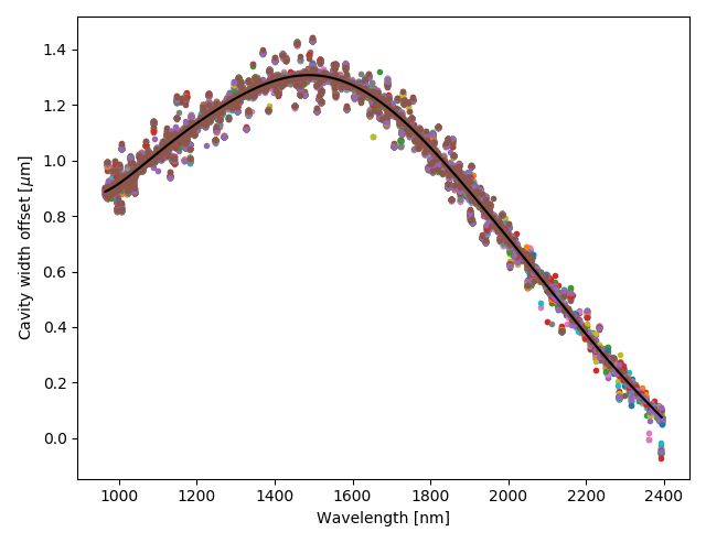
M. J. Hobson et al.: The SPIRou wavelength calibration for precise radial velocities in the near infrared

                                                                          Fig. 3. Comparison of wavelengths for common lines between the cata-
                                                                          logues of Redman et al. (2011) (R11) and Sarmiento et al. (2018) (S18).
Fig. 2. Raw SPIRou spectrum of the FP étalon (zoom to the same central    The blue points represent the difference in wavelengths, the black lines
region as Fig. 1). Light from the lamp is being fed to both the science   the S18 error bars. Points without error bars indicate that S18 reported
and calibration fibres. Around eight orders can be seen, centred around   no uncertainty for that line. The differences in wavelength are generally
1560 nm.                                                                  within the error bars when known, and always small.

                                                                          SPIRou run in February 20193 . The selected calibrations consist
solution during validation tests. In 2018, however, Sarmiento             of pairs of 1 HC (UNe) spectrum and 1 FP spectrum. The many
et al. (2018) (hereafter S18) published an updated catalogue of           instrument changes over the comissioning and early science runs
U lines in the 500 − 1700 nm wavelength range. While this is far          prevent us from making longer-term comparisons.
from covering the full wavelength range of SPIRou, encompass-
ing only the bluer half, it cross-matches well with the catalogue
of R11 (Fig. 3) and provides a substantial increase in the range          3. Methods
it does cover, incorporating 3787 new lines (median uncertainty
                                                                          3.1. SPIRou data reduction system
of all lines in the catalogue: 0.9 pm, translating to a median RV
uncertainty per line of 29 m s−1 ) for a total of 13554 lines in a        The wavelength solution is derived for each night as part of AP-
combined R11+S18 catalogue.                                               ERO (A PipelinE to Reduce Observations); APERO is main-
    For the ThAr lamp, the only catalogue that covered the                tained and version-controlled on github 4 . For the remainder of
SPIRou domain at the time was that of Redman et al. (2014)                this work we will refer to the SPIRou specific part of APERO as
(median uncertainty: 0.12 pm, translating to a median RV uncer-           the SPIRou data reduction system (DRS). The work presented
tainty per line of 7 m s−1 ). The UNe catalogue has far more lines        here was carried out primarily with version 0.5.000, which was
than the ThAr catalogue, even before the incorporation of the             released on 10 May 2019. The main differences with the current
lines from S18 (9767 vs 1587 in the SPIRou wavelength range).             development version are noted in Sect. 5, and will be described
                                                                          in a forthcoming paper (N.J. Cook et al. in prep).
    The laboratory tests performed at Toulouse, which are de-                 A full description of the DRS is beyond the scope of this
scribed in Perruchot et al. (2018), show that the UNe spectra             work, and will be done in N.J. Cook et al. (in prep). However, we
have around four times more identifiable lines than the ThAr              briefly summarise the calibration processing sequence for ver-
spectra, resulting in consistently more accurate and stable wave-         sion 0.5.000: pre-processing to remove certain detector effects
length solutions throughout the tests. Additionally, the ThAr             such as the amplificator crosstalk; generation of a dark calibra-
spectra show many more, and more strongly, saturated lines than           tion; creation of a map of the bad pixels, including two small
the UNe spectra in the SPIRou wavelength range. Saturated lines           holes and a scratch on the detector; localisation of the orders for
are useless for fitting a wavelength solution, since their cen-           fibres A, B, and C; mapping of the slit profile across the detector;
tres cannot be precisely determined. They will also ’bleed’ into          creation of the blaze profiles for all extracted fibres; generation
neighbouring orders and contaminate them. Additionally, persis-           of the wavelength map for all extracted fibres.
tence, which is a known problem for CMOS detectors such as the
H4RG (Artigau et al. 2018; Bechter et al. 2019), is stronger for
saturated lines, contaminating subsequent observations. There-            3.2. Wavelength solution using HC spectra alone
fore, the UNe lamp was adopted as the primary absolute wave-
                                                                          Two main methods were developed and tested for the wavelength
length calibrator.
                                                                          solution based on the HC lamp. The principal conceptual dif-
                                                                          ference between them lies in the way in which the HC lines
2.3. Selected datasets for testing                                        3
                                                                             All SPIRou calibrations are publicly available via the Cana-
                                                                          dian Astronomy Data Centre, at http://www.cadc-ccda.hia-iha.
To showcase the performance of the different methods devel-               nrc-cnrc.gc.ca/en/
                                                                          4
oped, we applied all the scripts on the calibrations of a two-week           Located at https://github.com/njcuk9999/apero-drs

                                                                                                                     Article number, page 3 of 12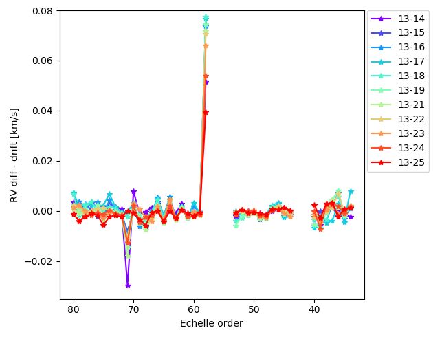
A&A proofs: manuscript no. main
are identified. The first, method HC1, is analogous to the SO- and stable wavelength solutions. For method HC1 in particular,
PHIE/HARPS wavelength solution (Baranne et al. 1996): For the SOPHIE/HARPS parameters were used as first guesses, and
each line in the catalogue, the region where it should be located modified as necessary. The fitted Gaussians to the HC lines have
is selected and a Gaussian fit is attempted, with poor fits being a median FWHM of 2.1 pixels, corresponding to wavelength val-
discarded. In the second, method HC2, Gaussians are fitted to ues ranging from 0.01 nm at the blue end of the spectrum to
every peak in the HC spectra, and the best match to the cata- 0.05 nm at the red end.
logue is identified. The detailed structure of the full routine is as
follows.
Fitting the solution: With the HC lines identified, a fourth-order
polynomial fit is performed for each order between the pixel po-
Data identification and reading: The input files are verified sitions given by the centres of the Gaussians, and the catalogued
via FITS header keys to be extracted two-dimensional spectra wavelengths. In method HC2, continuity of the polynomial coef-
(E2DS) corresponding to an HC lamp. The E2DS files con- ficients across the orders is also imposed at this step (attempts to
tain the extracted spectrum for a single fibre in the format of a impose similar cross-order continuity for method HC1 resulted
50 × 4089 array with one spectral order per row, arranged from in less stable solutions, so they were discarded).
blue to red. The data and header are read, and the lamp and fi-
bre are identified. If more than one HC file is given, the routine
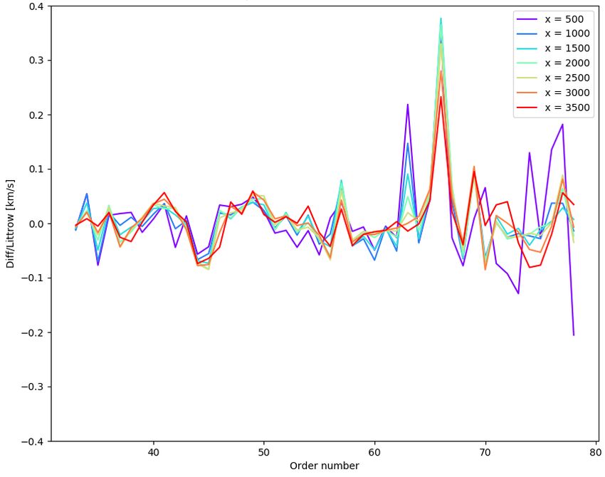
Littrow solution check: The Littrow check is a verification of
verifies they all correspond to the same lamp and fibre, then the
the cross-order continuity of the wavelength solution, following
median of the frames is obtained and used as input for the rest of
the same principles as in Cersullo et al. (2019). It is evaluated
the routine.
for several pixel positions (currently every 500 pixels along each
order in the dispersion direction). For each position x, a fourth-
Calibration set-up: The calibration files that are closest in time order polynomial fit is performed between the inverse echelle
to the input file(s) are copied from the calibration database (in- orders and the fractional wavelength contribution at x for each
cluding the previous wavelength solution). The previous wave- order (normalised by the wavelength for the first order), with an
length solution is read and checked for compatibility with the iterative step to remove the largest outlier. For an ideal spectro-
current parameter set-up (degree of the polynomial fits em- graph, the residuals to these fits would be zero. The polynomial
ployed, as this varied during development). The correct HC line fits, the residuals, and the minimum, maximum, and rms values
catalogue (UNe or ThAr) is read in. of the residuals are stored. An example is shown in Fig. 4.
Identification of the HC lines: The lines are identified following
one of the procedures outlined above:
Method HC1: For each line in the catalogue, a 4σ region in
wavelength (where σ is the expected width of the line, computed
from the central wavelength and the average spectral resolution)
around its expected position is selected, based on the previous
wavelength solution. A Gaussian fit to the region is attempted,
and kept if the σ of the fitted Gaussian is less than 4 km s−1 (to
discard very broad, flat lines whose centres will be imprecise),
and the amplitude is less than 1e8 (to avoid fitting on saturated
lines; we note that the amplitude is dimensionless as the E2DS
files are blaze-corrected within the routine).
Method HC2: For each spectral order, a 13-pixel-wide win-
dow is moved along the order in four-pixel shifts. If the max-
imum flux is at least at a 2σ level above the local RMS and
is within four pixels of the centre of the segment, a Gaussian
fit is attempted. The Gaussian is kept if the residual of the fit
normalised by the peak value is between 0 and 0.2 (to ensure
the fit is a good representation of the spectrum in that region), Fig. 4. Example Littrow solution check, showing the residuals of cross-
and the Gaussian σ in pixels, assuming a FWHM of 2 pixels, order fits between the inverse echelle orders and the fractional wave-
is between 0.7 and 1.1 (to discard narrow cosmic rays or broad length contribution. Each line corresponds to a different pixel position.
blended lines). Once all the peaks in the order are identified, the It should be noted that for the bluest orders, there is very little flux at
pixels 500 and 3500.
20 brightest (which are generally the least likely to be spurious,
and most likely to correspond to catalogued lines) are selected
and the closest catalogue line to each one is identified. Then, all
possible three-line combinations are used to fit a second-order Extrapolation of the reddest orders: For the last two orders,
polynomial to the order, test wavelengths are calculated for all very few HC lines are catalogued (13 in the last order, wave-
lines using the polynomial fit, and the velocity offset for each length range 2438-2516 nm, and 68 in the penultimate, wave-
from its identified catalogue line is calculated. The polynomial length range 2362-2437 nm, compared to an average of 300 for
with the most lines within 1 km s−1 of the catalogue is held to the rest) and even fewer are identified (around ten in the last
be the correct identification, and all peaks within 1 km s−1 of the order and 25 in the second-to-last for method HC2). This means
catalogue are kept. that the fitted solution often fails or is highly unstable. Therefore,
The parameter values were set and refined over the course for these orders it is not fitted from the HC lines, but extrapolated
of the pipeline development in order to obtain the most accurate from the Littrow solution: The cross-order polynomial fits are
Article number, page 4 of 12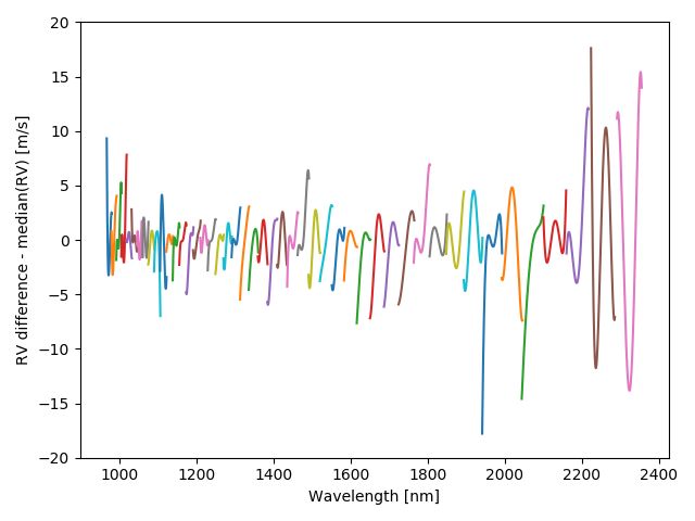
M. J. Hobson et al.: The SPIRou wavelength calibration for precise radial velocities in the near infrared

used to generate pixel-wavelength pairs at the Littrow evaluation         given by the FP equation (though we will see that for a physi-
positions, and these values are used in turn to fit a fourth-order        cal as opposed to an ideal étalon, this is not entirely accurate as
polynomial for each spectral order. A possible alternative would          the cavity width is wavelength-dependent). The absolute wave-
be to use telluric lines to fit these two orders; however, work           lengths of the FP lines, however, are not known but must be de-
by Figueira et al. (2010) using CRIRES suggests the precision             termined from some other source. Therefore, by anchoring the
would not be better than 5-10 m s−1 .                                     FP line wavelengths to the HC lines, we aimed to derive a more
                                                                          precise wavelength solution than could be obtained with the HC
                                                                          alone.
Quality controls: The structure of an E2DS file (one order per
row, wavelength increasing along the order) means that along                  In principle, the wavelength of an FP line is given by the FP
each column, the wavelength must be increasing - that is, each            equation:
pixel of order N must have a smaller wavelength value than the
corresponding pixel of order N+1. A first rough quality check,                   2d
                                                                          λm =      ,                                                        (1)
therefore, verifies that this is in fact the case (when this fails, it           m
generally points to a problem with the slit shape or order iden-
tification calibrations). A second quality check is applied to the        where λm is the wavelength of the line of (integer) line num-
minimum, maximum, and rms values of the Littrow check resid-              ber m, and d is the effective cavity width of the interferometer.
uals: The minimum and maximum must be within 0.3 km s−1 ,                 In an ideal FP interferometer, d is constant (and known since it
the rms within 0.1 km s−1 .                                               is set by the manufacturer); therefore, once the wavelength λm,r
                                                                          is known for a specific reference line, its line number mr can
Logging statistics: The mean and rms of the deviation from the            be determined. Then, for any other line, the line number can be
catalogued lines in m s−1 is logged, as is the total number of lines      determined simply by counting from the reference line, and its
used to fit the solution. Most importantly, the internal precision        wavelength calculated with Eq. 1. However, in real FP étalons,
of the solution is determined, as the rms of the residuals of the         the cavity width d is not constant. Bauer et al. (2015) showed it
fit to the catalogued lines, divided by the number of lines used to       to be wavelength-dependent, due to a varying penetration depth;
generate the fit.                                                         photons of different energy (i.e. different wavelength) will pene-
                                                                          trate the soft coating to different depths. This wavelength depen-
                                                                          dence needs to be calibrated in order to allow the use of the FP
Saving the solution: The wavelengths per pixel generated from             lines in a wavelength solution.
the polynomial fits for each order are saved as an E2DS file. The              Here, again, two methods were developed. The first, method
coefficients of the polynomial fits are stored in the header. If the      FP1, follows the approach described by Bauer et al. (2015): We
quality controls were all passed, the new wavelength solution is          first use the HC lines to generate a rough wavelength solution,
copied to the calibration database, and to the header of the input        from which we obtain first-guess FP wavelengths; these first-
HC E2DS spectra.                                                          guess wavelengths are in turn used to fit the cavity width. The
     Performance tests (discussed in more detail in Sect. 4.2)            second, method FP2, is based on the one developed by C. Lo-
showed that while the first method has slightly better internal           vis for ESPRESSO (private communication). Fractional FP line
accuracy than the second, it is much less stable night-to-night.          numbers are assigned to the HC lines, which are then used to fit
In any case, neither method reaches the expected internal accu-           the cavity width directly. The overall structure of the algorithm
racy of < 0.45 m s−1 budgeted for the SPIRou wavelength solu-             is as follows.
tion. The first method is also very sensitive to drifts from the ini-
tial wavelength solution (this was particularly highlighted by the
earthquake in May 2018, which caused a detector shift of several          Data identification and reading: The input files are verified via
pixels), to which the second method is more robust. The second            FITS header keys to be E2DS files corresponding to an HC lamp
method was therefore adopted for the HC wavelength solution,              and the FP étalon, respectively. The data and header are read, and
and is the only one available in version 0.5.000 of the DRS.              the lamp and fibre are identified. Fibre correspondence between
     During the SPIRou validation and commissioning tests, it be-         the HC and FP files is checked. If more than one HC file is given,
came clear that the HC lamps alone did not provide a sufficiently         the median of the frames is obtained and used as input for the rest
accurate and stable wavelength solution, with internal accuracy           of the routine. Currently, providing more than one FP file is not
measurements of ∼ 2-4 m s−1 compared to the 0.45 m s−1 accu-              supported. This option was chosen as allowing for multiples of
racy demanded by the SPIRou error budget for an overall 1 m s−1           each file type increased set-up complexity, and the FP spectra are
RV precision. There are likely several contributing factors to this       generally bright everywhere while the HC lines can be weaker.
lack of accuracy: the low flux levels in the edges of the bluest
orders, the low number of lines found for the reddest orders, im-
                                                                          Calibration set-up: Previous calibration files are copied from
precision in the catalogue wavelengths, among others. The next
                                                                          the calibration database (including the blaze file and the previous
step, therefore, was to combine the HC lamps with the FP étalon
                                                                          wavelength solution). The previous wavelength solution is read
spectra.
                                                                          and checked for compatibility with the current parameter set-
                                                                          up (order of the polynomial fits employed). The correct HC line
3.3. Wavelength solution combining HC and FP spectra                      catalogue is read in.
The design of the SPIRou FP étalon is described in Cersullo et al.
(2017). It has a finesse value of F = 12.8, and was designed to           Generation of a first-guess wavelength solution:         The HC
cover the entire 980 − 2350 nm wavelength range of SPIRou. Its            spectra are used to generate a wavelength solution, using Method
spectrum provides a wealth of lines across the entire detector,           HC2 from Sect. 3.2. Quality controls are applied to this first-
as shown in Fig. 2, whose spacing is a priori known since it is           guess solution.
                                                                                                                     Article number, page 5 of 12
A&A proofs: manuscript no. main

Incorporation of the FP lines: The FP lines are identified and           can be measured (by subtracting the RV of the wavelength so-
Gaussians fitted to them: For each order, the highest value is           lution’s FP from the RV of the simultaneous FP). Currently, we
identified, and a Gaussian fit attempted on a 7-pixel box around         assume the drift between the HC exposure that gives the abso-
it. Fits that do not fail and are centred within ±1 pixel of the         lute zero-point and an immediately subsequent FP exposure to
pixel with the highest value are stored, the rest are rejected. Fi-      be negligible, given the stability of SPIRou. In the future, a pos-
nally the Gaussian fit is subtracted (or the region set to zero if the   sible next step would be to employ HC-FP and FP-HC exposures
fit fails), and the process iterates until no more lines are found.      (i.e. exposures with the HC lamp on the science fibres and the FP
The Gaussians fitted to the FP have a median FWHM of 2.4 pix-            étalon on the calibration fibre or vice versa) to calibrate this drift,
els, corresponding to wavelength values ranging from 0.01 nm             as done in, for example, ESPRESSO or HARPS.
at the blue end of the spectrum to 0.05 nm at the red end. With
the FP lines’ pixel positions known, the initial wavelength solu-
                                                                         Littrow solution check, quality controls, logging statistics:
tion generated from the HC spectra alone is used to fit first-guess
FP wavelengths from the FP line pixel positions. Using the FP            These three steps are analogous to those of the HC solution.
equation and an input cavity width value, the FP line number
is obtained for the last peak of the reddest order. We initially         Saving the solution: Similar to the HC solution. If the qual-
used the manufacturer’s value of d = 12.25 mm before coating,            ity controls were all passed, the header of the input FP E2DS
meaning 2d = 24.5 mm, as the input value; subsequent testing             spectra is also updated. The HC and HC-FP solutions are stored
allowed us to refine it to 2d = 24.4999 mm. The rest of the lines        under different file names, so that the HC-FP solution does not
are then numbered by counting along each order, using wave-              overwrite the HC solution.
length matching across orders (with gaps due to missed peaks
accounted for). It does not matter whether the same last peak is
found for each observation, as we find that the variation of the         Saving results tables: Two tables are stored. The first logs the
cavity width within the order is small enough that the same FP           statistics of the Littrow solution quality check. The second is a
line numbers are obtained from the FP equation using the input           list of all lines used for the solution, containing the order, wave-
cavity width value as by counting from the last peak.                    length, difference in velocity of the final fit from the input line
                                                                         value, weight, and pixel position for each line.

Wavelength dependence of the cavity width: With the FP
line numbers identified, the wavelength dependence of the cavity
width is dealt with using one of the two methods named above:
    Method FP1: Using the line numbers and the first-guess
wavelengths of the FP lines (derived from the first-guess HC
solution previously generated), a cavity width is calculated for
each peak. A ninth-order polynomial is fitted to the cavity width
(Fig. 5, top points and fit), and corrected FP line wavelengths are
calculated from this polynomial fit.
    Method FP2: First, a fourth-order polynomial is fitted to the
FP line numbers as a function of pixel positions per order. This fit
is used to generate fractional line numbers for the ’best’ HC lines
(selected as the lines at blaze values of more than 30%, and with
velocity offset from the catalogue less than 0.25 km s−1 ). Using
these fractional line numbers and the catalogue wavelengths, the
cavity width is calculated for each HC line using the FP equation.
Ninth-order polynomials are then fitted to these cavity width val-       Fig. 5. Variability of the FP cavity width with regard to the input value
ues (Fig. 5, bottom points and fit) as a function of both line num-      for methods FP1 (FP lines) and FP2 (HC lines), offset by 0.5 µm for
ber and wavelength, and corrected FP line wavelengths are cal-           visibility (top), and residuals to the fits, offset by 0.05 µm for visibil-
                                                                         ity (bottom). The results from the two methods are very similar. For
culated from the fit. Optionally, a previous cavity width fit can be
                                                                         method FP1, some outliers (poorly fitted FP lines) can be seen, while
read in; in this case we assume only an achromatic change (i.e.          for method FP2 the number of lines drops off towards low line numbers
a shift) may have taken place, and correct the fit for this shift        (i.e. high wavelengths) and no lines are selected for the reddest order.
by subtracting the median of the residuals between the newly             For scale, a cavity width offset of 0.25 µm corresponds to a velocity
calculated cavity widths for the HC lines and the previous fit.          offset of 6.12 km s−1 , using the FP equation and the initial cavity width
                                                                         value of 2d = 24.4999 mm.

Fitting the solution: The HC and FP lines are combined. A                     As will be discussed in Sect. 4.3, the two methods are com-
fourth-order polynomial fit is performed between the pixel po-           parable, though method FP2 has slightly better accuracy and sta-
sitions, given by the centres of the Gaussians, and the line wave-       bility. In version 0.5.000 of the DRS, only method FP1 was avail-
lengths (catalogued for the HC lines, generated from the cavity          able for general use as method FP2 was still in development. In
width fit for the FP lines).                                             forthcoming versions both will be offered as options in the final
                                                                         wavelength solution algorithm.
Calculating the FP RV: The RV of the FP spectrum is cal-
culated using the cross-correlation function (CCF) method,               4. Performance tests and validation
through cross-correlation with an FP mask. It is stored in order
to give an FP RV zero-point, from which the drift of the spec-           To test the performance of the different wavelength solution gen-
trograph for a later observation of a star with simultaneous FP          eration methods, we ran all scripts on the calibrations of a two-
Article number, page 6 of 12
M. J. Hobson et al.: The SPIRou wavelength calibration for precise radial velocities in the near infrared
week SPIRou run in February 2019. We used three different UNe
line catalogues: the R11 catalogue, a combination of the R11
and S18 catalogues (with the S18 wavelengths kept for match-
ing lines), and a selection of the most stable lines (i.e. those con-
sistently identified for different HC frames) with updated, more
accurate wavelength values. This selection of lines was derived
using method FP2. First, the cavity width was fitted from the best
HC lines (at blaze values of more than 30%, and with velocity
offset from the catalogue less than 0.25 km s−1 ) for each of 50
HC exposures taken during commissioning (between May and
November 2018). For each of these exposures, the wavelengths,
fractional line numbers and calculated cavity widths of the lines
used for the fit were saved. Then, all the lines were combined,
and their wavelengths and cavity widths were fitted together to
generate a very accurate cavity width fit (Fig 6, top panel). Us-
ing this accurate cavity width fit, it can be seen that while for
each catalogue line the different cavity widths measured for each
exposure cluster together, these clusters can be significantly off-
set from the overall fit (Fig 6, bottom panel). This would mean
that for these offset values, the catalogue wavelengths are inac-
curate. Therefore, each measured line’s wavelength was recal-
culated from its fractional line number and the FP equation. Fi-
nally, each line that was selected in at least two exposures was
assigned an updated wavelength, as the median of its recalcu-
lated wavelengths. The stable lines catalogue is therefore not just
a selection of the best lines from the others, but a new catalogue
with updated wavelength values for each line. The full updated
catalogue is presented in Appendix 5.
4.1. Impact of previous calibrations
The wavelength solution is the last step of a long calibration se-
quence. This made its development particularly challenging as
changes upstream frequently meant large modifications in the
data that proved destabilising for the wavelength solution, es-
pecially in the earliest versions of the DRS. As the DRS has
evolved, this has somewhat ameliorated. Nevertheless, the pre- Fig. 6. Construction of a stable lines catalogue. Top: Overall cavity
vious calibrations can still impact the wavelength solution. In width fit (black line) from the HC lines (dots) for fifty exposures. Bot-
order to explore the performance of the wavelength solutions tom: Zoom showing how the values for each line cluster together, but
can be offset from the main fit. For scale, a cavity width offset of 0.2
alone, therefore, the tests presented in the rest of this section are
µm corresponds to a velocity offset of 4.88 km s−1 , using the FP equa-
all carried out with the HC and FP files extracted using a single tion and the initial cavity width value of 2d = 24.4999 mm.
set of input calibrations. We found that fixing the input calibra-
tions introduces large drifts between the wavelength solutions
for different nights, of the order of ∼ 10-50 m s−1 ; however, they a single spectral line. The ’HC lines used’ row is the median of
are easily calibrated out by subtracting the night-to-night me- the number of HC lines that were identified and used to fit each
dian RV difference. This removes sensitivity to long-term drifts, wavelength solution. The line count is performed per order, so
without affecting the analysis of the wavelength solution. any lines used for more than one order will be counted twice.
Method HC1 has better internal accuracy than method HC2,
4.2. Performances of the HC solutions but is less stable from one night to the next. As noted in Sect.
3.2, its sensitivity to the input wavelength solution was par-
To test the performance of the HC wavelength solutions, we ran ticularly highlighted by the earthquakes suffered by the CFHT
both methods on the UNe spectra taken as part of the afternoon during SPIRou validation, on 3 and 4 May 2018. The multi-
calibrations for the two-week SPIRou run in February 2019, for pixel displacement meant all lines were significantly shifted with
all three wavelength catalogues. The spectra were reduced with regard to the search windows defined from the previous (pre-
a single set of calibrations. We obtained one solution per night earthquake) solutions. This required the creation of additional
for each method and catalogue. Table 1 summarises the results. algorithms to identify the pixel shifts and generate shifted first-
The ’internal error’ row is a median of the internal accuracies re- guess solutions, in order for method HC1 to be able to run. Con-
ported for the solutions obtained with the corresponding method cern over this sensitivity was in fact one of the driving motiva-
and catalogue. The ’local night-to-night variation’ represents the tions for the development of method HC2, which (since it iden-
median difference between consecutive nights’ solutions (com- tifies all peaks in the spectrum and then generates a best match
puted as the median of the pixel-by-pixel absolute drift-corrected to the catalogue) is more robust to such shifts.
RV differences, with the drift corrected by subtracting the over- Regarding the catalogues, adding the lines from S18 does not
all median), and can be thought of as the typical uncertainty of seem to create a substantial change in accuracy or stability. Most
Article number, page 7 of 12A&A proofs: manuscript no. main
Table 1. Summary of HC wavelength solution performances.
Method HC1 Method HC2
R11 catalogue Global internal error 1.88 m s−1 3.87 m s−1
Local night-to-night variation 16.4 m s−1 6.3 m s−1
HC lines used 5607 4770
R11+S18 catalogue Global internal error 1.88 m s−1 3.95 m s−1
Local night-to-night variation 15.1 m s−1 7.6 m s−1
HC lines used 6186 5310
Selected lines Global internal error 1.46 m s−1 2.21 m s−1
Local night-to night variation 13.9 m s−1 5.7 m s−1
HC lines used 2363 2124
of the lines added have fairly low relative intensities reported by
S18, so they are likely small and their Gaussian fits may be less
precise. The ’stable lines’ catalogue provides somewhat more
accurate and stable wavelength solutions for both methods. In
any case, neither method reaches the required internal precision
of 0.45 m s−1 with any catalogue.
4.3. Performances of the HC+FP solutions
We used the same two-week SPIRou run in February 2019, pro-
cessed with a single set of calibrations, to test the performances
of both the combined HC-FP wavelength solution methods. To
generate the first-guess HC solution, we applied method HC2 in
both cases. Once again, we tested the three different wavelength
catalogues. Table 2 summarises the results, with the same rows
as for Table 1.
In this case, the two methods are very comparable, though
method FP2 has somewhat better internal accuracy and stabil- Fig. 7. Night-to-night variations of the FP wavelength solution: differ-
ence (in RV space) between the solutions generated with method FP2
ity. Rather perplexingly, for the combined HC-FP solutions the
for the 21 and 22 February 2019, using a fixed cavity width fit. The me-
’stable lines’ catalogue provides the least night-to-night stabil- dian value of the absolute RV differences is 0.8 m s−1 . The drift induced
ity! This is particularly evident for method FP2, where the HC by the fixed set of prior calibrations has been corrected.
lines are used to fit the cavity width directly. Since this catalogue
was generated from a cavity width fit using multiple HC expo-
sures, each reduced with the corresponding nightly calibrations,
this may perhaps be a derived effect of the previous calibrations’
instability. Nevertheless, in all cases the internal accuracy is ex- width fit, with the redder orders driving most of the remaining
cellent, and the night-to-night stability is much improved com- variability.
pared to the HC solutions.
As was described in Sect. 3.3, for method FP2 there is an
option to read in a previous cavity width fit and correct it from
any achromatic shift, instead of generating it anew. The reason- 4.4. Intra-night stability
ing behind this is that the chromatic dependence is an intrinsic
property of the soft coating; while it may evolve slowly over the To verify the intra-night stability of the HC-FP wavelength so-
lifetime of the instrument, it is not expected to change from one lution, we computed solutions using sequences of 1 HC and 10
night to the next. An achromatic shift, meanwhile, would cor- FP frames taken continuously over a 14h period. We adopted
respond to a change in the physical separation of the FP, which two test configurations: fixing the HC frame and varying the FP
could be caused by pressure or temperature changes. frame, and fixing the FP frame and varying the HC frame. For
We tested the implementation of this option, redoing the each of these, we obtained HC-FP wavelength solutions using
analysis with an initial cavity width read in. We found a me- method FP2. We then computed the RV of an FP frame (taking
dian internal error of 0.14 m s−1 , and a median night-to-night it as an artificial ’star’) using the different wavelength solutions.
variation of 0.8 m s−1 , regardless of the catalogue used. This im- The resulting RV variations (corrected for the spectrograph drift
plies that a substantial part of the night-to-night variability for by using the FP calibration fibre CCF, as described in Section
the combined HC-FP solutions is in fact coming from the cavity 3.3) are shown in Fig. 8. For the case of a fixed HC frame and
width fit. An example of a night-to-night comparison is shown varying FP frames, the RV variations show a slow downward
in Fig. 7, for the solutions computed with method FP2 using trend, which is probably due to the intrinsic drift of the FP étalon
a fixed cavity width, for the nights of 21st and 22nd February with respect to the absolute wavelength reference. For the case
2019, respectively. The night-to-night variations are significantly of a fixed FP frame and varying HC frames, the RV variations are
reduced compared to the solutions obtained with a free cavity very small, with an amplitude comparable to the photon noise.
Article number, page 8 of 12M. J. Hobson et al.: The SPIRou wavelength calibration for precise radial velocities in the near infrared
Table 2. Summary of HC-FP wavelength solution performances.
Method FP1 Method FP2
R11 catalogue Global internal error 0.18 m s−1 0.12 m s−1
Local night-to night variation 3.1 m s−1 1.5 m s−1
HC+FP lines used 23612 21662
R11+S18 catalogue Global internal error 0.18 m s−1 0.12 m s−1
Local night-to night variation 3.0 m s−1 1.9 m s−1
HC+FP lines used 23691 21874
Selected lines Global internal error 0.18 m s−1 0.13 m s−1
Local night-to night variation 4.3 m s−1 3.3 m s−1
HC+FP lines used 22990 20466
Fixed cavity width Global internal error NA 0.14 m s−1
Local night-to night variation NA 0.8 m s−1
served spectrum. This cross-correlation is first performed order
by order; these are then summed together, and a Gaussian fit
is performed, the final RV being measured as the centre of the
Gaussian. The RVs per order and the combined RV are all stored.
If the star is observed with simultaneous FP on the calibration fi-
bre, the instrumental drift is computed by the same recipe, cross-
correlating the FP spectrum to a binary FP mask.
To evaluate the impact of the wavelength solution on the
RVs, we selected observations of two stars, which we shall refer
to as star A and star B, chosen as they are the brightest targets
observed close to the centre of the February 2019 run. For each
star, we computed the RVs changing the input wavelength solu-
tion. To generate the wavelength solutions, we adopted method
FP2 and a fixed cavity width fit as this was shown to provide the
most accurate and stable set of wavelength solutions. We used
the CCF computation from the SPIRou DRS to obtain the RVs.
Both stars were observed with simultaneous FP calibration, so
the drift was also computed from the FP CCFs, as described in
Section 3.3. The results are summarised in Table 3. The standard
deviation of the differences from the RV obtained for 13 Febru-
ary (taken as the reference point) is 0.67 m s−1 for star A, and
0.40 m s−1 for star B. We observed and corrected for large drifts
(median value 11.5 m s−1 ); these drifts are induced by the fact we
have fixed a single set of prior calibrations for extracting all the
files, which creates offsets between the wavelength solutions, as
described in Sect. 4.1. The physical origin of these day-to-day
drifts may lie in many different factors: The instrument is known
to be sensitive to vibrations; the room in which the FP is located
is not stabilised; there are known jumps at each thermal cycle of
the cryostat; among others.
Although the overall variations are small, it is worthwhile to
inspect the CCFs in more detail. Fig. 9 shows the drift-corrected
difference in CCF RVs per order for each star. Gaps correspond
to orders for which no CCF could be calculated (generally due to
a very low or null atmospheric transmission). It is clear that some
Fig. 8. Radial velocity variations over time for a CCF RV of an FP orders are far more variable than others, and may be driving the
frame (taking it as an artificial ’star’), computed using wavelength so- RV differences. It is hard to say whether this is due to solely to
lutions with a fixed HC frame and varying FP frames (top), or varying the wavelength solution (since, for instance, Fig. 7 does not show
HC frames and a fixed FP frame (bottom). The RVs have been drift- significantly higher night-to-night variability in these orders), or
corrected.
whether there are also factors due to the CCF at play (e.g. smaller
spectral lines in these orders whose fit could be more impacted
by small shifts in wavelength solution).
4.5. Impact on RV error
In particular, for star A the RVs for echelle orders 71 (cen-
Ultimately, the interest of an accurate and stable wavelength so- tral wavelength 1097 nm) and 79 (central wavelength 984 nm)
lution for a spectrograph lies in being able to measure precise have standard deviations of ∼ 5 m s−1 , while the rest are below
RVs. In the SPIRou DRS, RVs are measured by the CCF method ∼ 3 m s−1 . Likewise, for star B, the RVs for echelle orders 58
- that is, by cross-correlating a binary stellar mask with the ob- (central wavelength 1348 nm) and 71 have standard deviations
Article number, page 9 of 12A&A proofs: manuscript no. main
Table 3. Summary of CCF RV differences using different wavelength solutions.
Star Wavelength RV diff (all RV diff (sel.
sol. night orders) [m s−1 ] orders) [m s−1 ]
star A 13 Feb — —
14 Feb 0.89 0.89
15 Feb 0.20 0.20
16 Feb 0.22 0.22
17 Feb 0.68 0.68
18 Feb 0.26 0.25
19 Feb 0.36 0.35
21 Feb -0.39 -0.40
22 Feb 0.07 0.07
23 Feb 0.09 0.09
24 Feb -0.54 -0.55
25 Feb 1.93 -0.78
σRVdi f f 0.67 0.50
star B 13 Feb — —
14 Feb 1.01 1.01
15 Feb 0.20 0.23
16 Feb 0.07 0.10
17 Feb -0.61 -0.58
18 Feb 0.14 0.17
19 Feb 0.39 0.42
21 Feb 0.18 0.19
22 Feb 0.08 0.10
23 Feb 0.22 0.23
24 Feb -0.09 -0.08
25 Feb -0.20 -0.20
σRVdi f f 0.50 0.39
of ∼ 12 m s−1 and ∼ 8 m s−1 respectively, while the rest are below tions, especially on the slit determination. Fixing all prior cali-
∼ 3 m s−1 . For order 58 for star B, in particular, closer analysis brations produces a noticeable (∼ 10-50 m s−1 ) but constant RV
shows the Gaussian fit to the CCF is clearly poor, explaining the offset between solutions; when this offset is removed, the night-
high RV offset and dispersion. Recalculating the RVs excluding to-night variations are greatly diminished. We analysed the im-
the worst two orders for each star, the differences are generally pact of changing the wavelength solution on the RV calcula-
slightly reduced (last column of Table 3), with a standard devia- tions, finding that the calculated RVs remain fairly consistent
tion of 0.50 m s−1 for star A and 0.39 m s−1 for star B, though the with ∼ 0.5-0.7 m s−1 dispersions, and that the drift computation
impact is not large. is efficient at removing the RV offset between wavelength solu-
There are many factors that may contribute to the remaining tions computed with a fixed set of previous calibrations.
noise. The photon noise is at the ≤ 0.10 m s−1 level, so is un- This article is based primarily on the current stable version
likely to be a major contributor. The spectrograph drift correc- of the DRS, 0.5.000. Significant changes have been planned for
tion may be playing a role (over 12 days, the drift is of the order future versions, which the DRS team is currently working on.
of ∼ 50 m s−1 . In standard operations with daytime calibrations, Several of these changes are either directly on the wavelength
these drifts would not appear; as we fixed a single set of calibra- solution, or are expected to impact it, such as the implementation
tions, they need to be removed separately). For the wavelength of a set of ’master’ calibrations that are not expected to change
solution, inaccuracies in the UNe catalogues and fit instabilities on a nightly basis, but only per run or even per thermal cycle.
may increase the noise. Several detector-related effects may also One of these master calibrations will be a master wavelength so-
be contributing, such as cosmic rays, bad pixels, the known per- lution, with nightly calibrations measuring only the offset from
sistence on H4RG detectors, or intra-pixel response variations. this master solution. Another problem to be dealt with is poten-
tial variations between solutions obtained for the science and cal-
ibration fibres. In version 0.5.000, these are computed indepen-
5. Conclusions and future perspectives dently, which can lead to cases such as the wavelength solution
We have implemented and tested different methods of generat- failing quality controls for one fibre but not another. Upcoming
ing a wavelength-pixel correspondence, using either HC lamps versions will anchor the calibrations together to avoid this prob-
alone or the combination of HC lamps with an FP étalon. The lem.
HC lamps alone did not provide sufficient accuracy, being at the Wavelength solutions combining HC and FP exposures are
level of ∼ 2-3 m s−1 internal error, while the error budget pre- implemented for CARMENES (Bauer et al. 2015; Caballero
vision was of < 0.45 m s−1 . The combined HC-FP solutions, on et al. 2016) and have recently been tested for HARPS (Cersullo
the other hand, have an excellent internal error of ∼ 0.15 m s−1 . et al. 2019). In both cases, these wavelength solutions are shown
The stability from one night to the next is complicated by the to be suitable for reaching a 1 m s−1 overall RV precision. We
dependence of the wavelength solution on the previous calibra- anticipate that this will also be the case for SPIRou.
Article number, page 10 of 12M. J. Hobson et al.: The SPIRou wavelength calibration for precise radial velocities in the near infrared
Fig. 9. Drift-corrected CCF RV differences per order for star A (left) and star B (right), using wavelength solutions from different nights. The
strong variations of echelle order 58 for star B are due to a poor CCF fit.
Acknowledgements. The authors wish to recognise and acknowledge the very Cersullo, F., Wildi, F., Chazelas, B., & Pepe, F. 2017, A&A, 601, A102
significant cultural role and reverence that the summit of Maunakea has always Coffinet, A., Lovis, C., Dumusque, X., & Pepe, F. 2019, A&A, 629, A27
had within the indigenous Hawaiian community. We are most fortunate to have Donati, J.-F., Kouach, D.and Moutou, C., Doyon, R., et al. submitted
the opportunity to conduct observations from this mountain. This work was sup- Donati, J.-F., Kouach, D., Lacombe, M., et al. 2018, SPIRou: A NIR
ported by the Programme National de Planétologie (PNP) of CNRS/INSU, co- Spectropolarimeter/High-Precision Velocimeter for the CFHT, 107
funded by CNES. We acknowledge funding from ANR of France under contract Figueira, P., Pepe, F., Melo, C. H. F., et al. 2010, A&A, 511, A55
number ANR-18-CE31-0019 (SPlaSH). This research made use of matplotlib, Fischer, D. A., Anglada-Escude, G., Arriagada, P., et al. 2016, PASP, 128,
a Python library for publication quality graphics (Hunter 2007); SciPy (Jones 066001
et al. 2001–); IPython package (Pérez & Granger 2007); Astropy, a community- Ginsburg, A., Sipőcz, B. M., Brasseur, C. E., et al. 2019, AJ, 157, 98
developed core Python package for Astronomy (Astropy Collaboration et al. Halverson, S., Mahadevan, S., Ramsey, L., et al. 2014, Society of Photo-
2018, 2013); NumPy (Van Der Walt et al. 2011); Astroquery (Ginsburg et al. Optical Instrumentation Engineers (SPIE) Conference Series, Vol. 9147, The
2019); ds9, a tool for data visualisation supported by the Chandra X-ray Sci- habitable-zone planet finder calibration system, 91477Z
ence Center (CXC) and the High Energy Astrophysics Science Archive Center Hunter, J. D. 2007, Computing In Science & Engineering, 9, 90
(HEASARC) with support from the JWST Mission office at the Space Telescope Jones, E., Oliphant, T., Peterson, P., et al. 2001–, SciPy: Open source scientific
Science Institute for 3D visualisation. We thank all SPIRou partners for their tools for Python, [Online; accessed ]
funding contributions to the SPIRou project, whose construction cost (includ- Kokubo, T., Mori, T., Kurokawa, T., et al. 2016, Society of Photo-Optical Instru-
ing reviews and travels) reached a total of 5Me, namely the IDEX initiative at mentation Engineers (SPIE) Conference Series, Vol. 9912, 12.5-GHz-spaced
UFTMP, UPS, the DIM-ACAV programme in Region Ile de France, the MIDEX laser frequency comb covering Y, J, and H bands for infrared Doppler instru-
initiative at AMU, the Labex@OSUG2020 programme, UGA, INSU/CNRS, ment, 99121R
CFI, CFHT, LNA, CAUP and DIAS. We are also grateful for generous amounts Kotani, T., Tamura, M., Nishikawa, J., et al. 2018, in Society of Photo-Optical
of in-kind manpower allocated to SPIRou by OMP/IRAP, OHP/LAM, IPAG, Instrumentation Engineers (SPIE) Conference Series, Vol. 10702, Proc. SPIE,
CFHT, NRC-H, UdeM, UL, OG, LNA and ASIAA, amounting to a total of about 1070211
75 FTEs including installation and ongoing upgrades. This work has been car- Lovis, C. & Pepe, F. 2007, A&A, 468, 1115
ried out within the framework of the National Centre of Competence in Research Marcy, G. W. & Butler, R. P. 1992, PASP, 104, 270
PlanetS supported by the Swiss National Science Foundation. Murphy, M. T., Udem, T., Holzwarth, R., et al. 2007, MNRAS, 380, 839
Pérez, F. & Granger, B. E. 2007, Computing in Science and Engineering, 9, 21
Perruchot, S., Hobson, M., Bouchy, F., et al. 2018, in Society of Photo-Optical
Instrumentation Engineers (SPIE) Conference Series, Vol. 10702, 1070265
References Quirrenbach, A., Amado, P. J., Ribas, I., et al. 2018, in Society of Photo-Optical
Instrumentation Engineers (SPIE) Conference Series, Vol. 10702, Proc. SPIE,
Artigau, É., Kouach, D., Donati, J.-F., et al. 2014, in Proc. SPIE, Vol. 9147, 107020W
Ground-based and Airborne Instrumentation for Astronomy V, 914715 Redman, S. L., Lawler, J. E., Nave, G., Ramsey, L. W., & Mahadevan, S. 2011,
Artigau, É., Saint-Antoine, J., Lévesque, P.-L., et al. 2018, in Society of Photo- ApJS, 195, 24
Optical Instrumentation Engineers (SPIE) Conference Series, Vol. 10709, Redman, S. L., Nave, G., & Sansonetti, C. J. 2014, ApJS, 211, 4
Proc. SPIE, 107091P Sarmiento, L. F., Reiners, A., Huke, P., et al. 2018, A&A, 618, A118
Astropy Collaboration, Price-Whelan, A. M., Sipőcz, B. M., et al. 2018, AJ, 156, Spronck, J. F. P., Fischer, D. A., Kaplan, Z., et al. 2015, PASP, 127, 1027
123 Van Der Walt, S., Colbert, S. C., & Varoquaux, G. 2011, Computing in Science
Astropy Collaboration, Robitaille, T. P., Tollerud, E. J., et al. 2013, A&A, 558,
& Engineering, 13, 22
A33
Wildi, F., Pepe, F., Chazelas, B., Lo Curto, G., & Lovis, C. 2011, Society
Baranne, A., Queloz, D., Mayor, M., et al. 1996, A&AS, 119, 373
Bauer, F. F., Zechmeister, M., & Reiners, A. 2015, A&A, 581, A117 of Photo-Optical Instrumentation Engineers (SPIE) Conference Series, Vol.
Bechter, E. B., Bechter, A. J., Crepp, J. R., & Crass, J. 2019, arXiv e-prints, 8151, The performance of the new Fabry-Perot calibration system of the ra-
arXiv:1908.11429 dial velocity spectrograph HARPS, 81511F
Boisse, I., Perruchot, S., Bouchy, F., et al. 2016, in Society of Photo-Optical In-
strumentation Engineers (SPIE) Conference Series, Vol. 9908, Ground-based
and Airborne Instrumentation for Astronomy VI, 990868
Butler, R. P., Marcy, G. W., Williams, E., et al. 1996, PASP, 108, 500
Caballero, J. A., Guàrdia, J., López del Fresno, M., et al. 2016, in Society
of Photo-Optical Instrumentation Engineers (SPIE) Conference Series, Vol.
9910, Proc. SPIE, 99100E
Cersullo, F., Coffinet, A., Chazelas, B., Lovis, C., & Pepe, F. 2019, A&A, 624,
A122
Article number, page 11 of 12You can also read